Decomposition and Conceptualization to Support System Dynamics Behavior Modeling

Complex Systems Informatics and Modeling Quarterly (CSIMQ) eISSN: 2255-9922

Published online by RTU Press, https://csimq-journals.rtu.lv Article 88, Issue 15, June/July 2018, Pages 45–71

https://doi.org/10.7250/csimq.2018-15.03

Decomposition and Conceptualization to Support System Dynamics

Behavior Modeling

Fiona Tulinayo1?_{, Theo van der Weide}2_{, and Patrick van Bommel}2

1_{Makerere University, College of Computing and Information Sciences, Uganda} 2_{Radboud University, Institute of Computing and Information Sciences, the Netherlands}

fturinayo@cit.ac.ug,tvdw@cs.ru.nl,pvb@cs.ru.nl

Abstract. With the increasing need for data-based decision making, social

systems and the ecosystems; practitioners and decision makers need guid-ance in their decision making, as is offered by data-based models and a sys-tematic generation of simulation tools. Overtly, relations between data and practice have been under-conceptualized. Data modelers and decision mak-ers tend to lack a mutual undmak-erstanding of each other’s knowledge systems which has led to huge knowledge gaps. Assimilation of modeling methods therefore is vital. Modeling methods use a specific way of thinking, rules and directions on how to model different aspects of systems. These rules and directions are what we refer to as constructs. Conceptualizing model re-lations and formure-lations requires significant domain knowledge and under-standing of the constructs. In this article, we use the decomposition mech-anism to better conceptualize and understand the System Dynamics (SD) model behavior, and show how using a natural language based domain mod-eling method (Object-Role Modmod-eling, ORM) helps in dealing with complex SD models. Through applying the decomposition mechanism, we are able to better understand the underlying concepts of the stock and flow diagram and update behaviors of ORM objects. To achieve this, we use examples and an SD model derived from a case “Intrapartum process in Ugandan hospi-tals” to study the object behaviors. The main results of this article include: a theoretical founding of integrating ORM with SD; quantitative analysis at the level of ORM reasoning; and transformation rules from ORM into SD.

Keywords: System Dynamics, Constructs, Decomposition, Object-Role

Modeling.

1

Introduction

Complex systems are characterized by a large number of interacting elements whose overall char-acteristics cannot be deduced directly from their components. The behaviour of these systems usually is too complex to be modeled by a set of differential equations. Usually, policy makers want to understand these systems sufficiently to develop policies intended to attain optimal system

?_{Corresponding author}

c

2018 Fiona Tulinayo et al. This is an open access article licensed under the Creative Commons Attribution License (http://creativecommons.org/licenses/by/4.0).

Reference: F. Tulinayo, Th. van der Weide, and P. van Bommel, “Decomposition and Conceptualization to Support System Dynamics Behavior Modeling,” Complex Systems Informatics and Modeling Quarterly, CSIMQ, no. 15, pp. 45–71, 2018. Available: https://doi.org/10.7250/csimq.2018-15.03

behaviour. This may be seen as a complex decision problem. Modeling and simulation is increas-ingly used to provide some understanding that helps policy makers to find such optimal policies.

The analysis of such systems typically requires an interdisciplinary approach combining math-ematical and computing science methods with those of environmental, economic, biological and social sciences, often finding a serious gap between the domain’s and the ICT languages and meth-ods to bridge.

The increased need for data-based decision making and data integration also requires the com-bining of various modeling methods [1]. Modeling methods each use a specific way of thinking, rules and directions on how to model an aspect of a system [2]. These rules and directions are what we refer to as constructs. Constructs specify what can be modeled with a given method and define the world view of the method [3]. Here, we use the term constructs as concepts, ideas or images specifically conceived for the purpose of organizing and representing knowledge of interest of a given modeling method [4]. In [5] Wieringa states that understanding the underlying ideas of different methods helps in defining their transition and relations. Yet, understanding relations and formulations requires significant domain knowledge and understanding of the constructs for both the source and target modeling methods. That is to say, the source modeling method constructs are transformed into target modeling method constructs by applying a set of transformation rules. The transformation rules are the smallest entity within a model transformation. They describe how a fragment of the source model can be transformed into a fragment of the target model [6]. Here, we equate fragments to constructs. Putting these fragments together makes a complete set of constructs for a specific modeling method. The transformation rules therefore, help in describing how one or more constructs in the source modeling method can be transformed into one or more constructs in the target modeling method [6]. By understanding the different constructs and transformation rules, constructing a new viewpoint model based on the existing models is realized [7]. For proper model synchronization, it is urged that transformations should consistently propagate changes between different model constructs [8].

The intention of this article is to propose a combination of methods that (1) produces domain descriptions that are understandable by a non-technical domain expert (2) allows for a concise description of complex domains and (3) can be systematically transformed into a simulation tool. In order to be understandable by the domain expert, the method (1a) should be able to handle complexity, and (1b) is communicable at the level of the domain expert.

A major issue during modeling and design is to reduce complexity by introducing various levels of understanding. A most popular method is the decomposition mechanism. This mecha-nism has been widely applied in different fields, e.g. in method engineering [9], in dynamic mode decomposition (DMD) [10] and in process models [11]. In this article we use the decomposition mechanism to better conceptualize and understand the System Dynamics (SD) model behavior, and show how using a domain modeling method (Object-Role Modeling (ORM)) helps in constructing understandable (and thus valid) SD models.

dynamic phenomena than CLDs [15]. SFDs bring together the modeler’s creative thinking ability and their data manipulation ability because they add the dimension of data to mapping of structures which then leads to computer simulation of systems to ascertain the model behavior over time [16]. The derived simulations provide quantitative estimates of system effects and as such, models can be used in a “what if” mode to experiment with alternative configurations, flows and resources [17]. Within the SD community there is consensus on the importance of qualitative data during the development of a system dynamics model, but there is not a clear description about how or when to use it. The lack of a defined systematic procedure on how to obtain and analyze qualitative in-formation creates a gap between the problem modeled and the model of the problem. This causes difficulty in “understanding the links between the observations of reality and the assumptions or formulations in the model especially when the model contains soft variables” [18].

In [19], we noted that SD lacks instruments for discovering and expressing precise language based concepts in domains yet conceptual/domain modeling has long focused on deriving models from natural expressions. In this article therefore, we try to understand the system dynamics rela-tions between observarela-tions of reality and formularela-tions through a domain data modeling method, Object-Role Modeling (ORM). We use ORM in particular as an example of a domain modeling language because of its conceptual focus and roots in verbalization, graphical expressiveness and well-defined semantics. The philosophy behind ORM is that it tries to describe a Universe of Dis-course (UoD) by describing the communication between its members. An ORM scheme basically is a grammar describing that communication. This grammar is also referred to as information gram-mar. The general construction of an information grammar is as follows. There is a set of syntactic categories (in ORM terminology: object types) and a set of grammar rules (in ORM terminology: fact types) that describe how these syntactic categories are constructed from other syntactic cate-gories. A grammar rule basically indicates the object types involved in a fact type and in what role. The term predicator is used to indicate such a role. Therefore, in ORM a fact type is seen as a set of roles. The information grammar describes the elementary sentences that are valid in the asso-ciated UoD. From these sentences other sentences may be formed. Object Role Calculus (ORC) [20] and ORM2 [21] are examples of such generic systems for constructing sentences. These sen-tences will be referred to as information descriptors. The notion of information descriptors was introduced under LISA-D (Language for Information Structure and Access Descriptions) which is based on PSM (Predicator Set Model) in [20]. With respect to decomposition, the data modeling technique PSM [20] introduces theschema typeas a mechanism for decomposition. Besides PSM introduces the grammar type for semi-structured data, allowing the PSM schema to be extended with a grammatical description (which can be compared to a DTD in XML). However, PSM does not cater for the behavioral description of objects. In [22] abstraction layers for data modeling are introduced at a more fundamental level. Several additional methods have been proposed to com-bine data modeling with behavioral descriptions, such as state charts (see for example [23]). UML (see for example [24]) offers modeling techniques for many aspects of software development, such as a class model and behavior description. PSM2 _{([25]) is an action-based approach to model an}

application domain, starting from a sample behavioral description (called a logbook, see [26]). PSM2_{does not have a mechanism for decomposition in the behavioral description of object types.}

For similar applications, see [27], [28] and [29].

Demon-stration: Demonstrate the use of the artifact to solve one or more instances of the problem. This could involve its use in experimentation, simulation, case study, proof, or other appropriate activ-ity. 5. Evaluation: Observe and measure how well the artifact supports a solution to the problem. Depending on the nature of the problem venue and the artifact, evaluation could take many forms. 6. Communication: Communicate the problem and its importance, the artifact, its utility and nov-elty, the rigor of its design, and its effectiveness to researchers and other relevant audiences, such as practicing professionals, when appropriate. Our work is organized in accordance with these 6 steps as follows. Problem identification and motivation and the definition of the objectives for a solution are described in the introduction of this article. Design and development are the topic of Sections 3 and 4. Sections 5 and 6 provide a demonstration of the proposed method. The conclu-sion of this article addresses the evaluation of the method proposed in this article. The final step, communication, can be found throughout the article.

The rest of this article proceeds as follows. In Section 2, we present the basic concepts and constructs of the domain modeling method under consideration (ORM). We use the decomposi-tion mechanism of this method to define the SD method. Therefore, we present SD constructs with their underlying principles in Section 3. In order to achieve a solid theoretical founding of inte-grating ORM with SD, we start by presenting causal loop diagram constructs and their underlying principles, along with formal definitions of causal loop diagrams in Subsection 3.1. Next we con-sider stock and flow diagrams in Subsection 3.2. The corresponding quantitative analysis at the level of ORM reasoning is presented in Section 4. Our approach has been applied in a real life con-text, which is described in Section 5. Here, we use the case study Intrapartum process in Ugandan Hospitals to demonstrate that these ORM and SD concepts facilitate ORM to work as a foundation for SD. After constructing the model, it is decomposed by first separating the object types and then treating each object type independently. This leads to the definition of all influencing relations. In Section 6 the design from Section 5 is realized with a concrete SD tool. In Section 7 we shortly evaluate the merits of our proposed method, draw some conclusions, and suggest some further research, directions.

2

ORM Concepts and Constructs

ORM’s basic building blocks include: entity types (object types), value types and roles [32]3_{. An}

object type is a collection of objects with similar properties, in the set-theoretical sense.Objects

are things of interest, they are either instances of entity or value types. Entity types are designated by solid-line named ellipses in the graphical reproduction of the information grammar. All entity types have a reference scheme, which may be simple (either a reference mode, or an entity to entity relationship) or compound. These reference schemes indicate how a single value relates to that entity type. Value types, on the other hand, have instances with a universally understood denotation, and hence require no reference scheme. They are identified solely by their values, their state never changes and they are designated by dotted ellipses. The semantic connections between object types are depicted as combinations of boxes and are calledfact types. Each box represents a role and is connected to an object type or a value type. The roles denote the way entity types participate in that fact type. The number of roles in a fact type are referred to asfact type arityand the semantics of the fact type are put in a fact predicate. A predicateis basically a sentence with object holes in it, one for each role. These predicate names are written beside each role and are read from left to right, or top to bottom. It is through predicates that entity types relate to each other. To represent some of these definitions let us use an example of the procedures a patient might go through en route from arrival to discharge. The procedures are stated as:

S1 Patient (Name) arrives at Hospital (Name) at Time (.am/p.m.). S2 Patient (Name) queues up.

3_{For ORM terminologies in this study, we used Halpin and Morgan [32]; and to model ORM models we}

S3 MedicalPerson (Name) examines Patient (Name) to establish Patientillness (Name). S4 Patient (Name) is treated by MedicalPerson (Name).

S5 Patient (Name) is discharged by MedicalPerson (Name).

Patient

Patient arrival

Patient Treated

Patient Discharged Patient examined Patient in queue Arrives

Queues up

Is examined

Receives treatment

Is discharged

Patient

Arrival Queues up Is examined Is treated Is discharged

S1 S2 S3 S4 S5

Figure 1.Various Patient states

The procedure presented in Figure 1 basically describes the various subsequent states recog-nized for the object type Patient. In this article, we further explore the notion of state presented in Figure 1, and how states come in naturally during the modeling process. The conceptual structure of this example is represented on an ORM diagram in Figure 2.

 

C

2

 

C

1

C

5

C

4

C

3

Figure 2.ORM Patient flow concepts

C1 (Exclusive or):For eachPerson,exactly one of the following holds:

somePatient isthatPerson;someMedical Person isthatPerson.

C2 (Subset)If somePatient is in queuethen thatPatient arrives atsomeHospital atsomeTime.

C3 Medical Person examines Patient.It is possible that more than oneMedical Person examines

the samePatientand that more than onePatient is examined bythe sameMedical Person. Each Patient is treated by at most one Medical Person.

C4 If someMedical Person treatssomePatientthen thatMedical Person dischargesthatPatient.

C5 (mandatory):eachPatient is discharged byat least oneMedical Person.

3

SD Constructs and Underlying Principles

As already stated, the SD notations (CLDs and SFDs), each have a number of constructs with underling principles4. In subsections 3.1 and 3.2 respectively, we present their basic building blocks and underlying principles.

3.1 Constructing a Causal Loop Diagram

A Causal Loop Diagram is made up of variables, signs (either a positive or negative) and causal

links with arrows representing the causal influence. The arrows are drawn in a circular manner

indicating the cause and effect leading to a feedback loop which is a closed sequence of causes and effects sometimes referred to as a closed path of action and information [33]. When constructing a CLD, there are design rules to be followed.

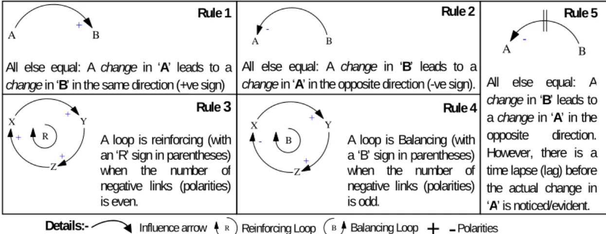
Design Rule 1 (Positive sign): A causal link from one element ‘A’ to element ‘B’ is positive

(+)if either ‘A’ adds to ‘B’ or a change in ‘A’ makes variable ‘B’ change in thesamedirection.

Design Rule 2 (Negative sign):A causal link from one element ‘A’ to another element ‘B’ is

negative (-) if either ‘A’ subtracts from ‘B’ or a change in ‘A’ makes ‘B’ change in the opposite

direction. In addition to the signs on each link, is a complete loop sign (either a positive (Reinforc-ing) or negative (Balanc(Reinforc-ing). The sign for a particular loop is determined by counting the number of minus (-) signs on all the links that make up that loop.

Design Rule 3 (Reinforcing Loop):A feedback loop is calledpositive or reinforcing, indicated by a plus or‘R’sign in parentheses, if it contains an even number of negative causal links.

Design Rule 4 (Balancing Loop):A feedback loop is callednegative or balancing, indicated by a minus or‘B’sign in parentheses, if it contains an odd number of negative causal links.

Thus, the sign of a loop is the algebraic product of the signs of its links. Often a small looping arrow is drawn around the feedback loop sign to more clearly indicate that the sign refers to the loop (see Rule 3 and 4 in figures presented in Figure 3). Further explanation on how CLD influences operate can be found in [12].

Design Rule 5 (Delay Mark/Time Delay):Between variables ‘B’and‘A’ in Rule 5, Figure 3, is a delay mark. This delay mark implies that there is a time lapse (lag) between these variables before the actual change is noticed or becomes evident. Delays are of two types: material delays and information delays. Material delays represent a lag in the physical flow while information delays represent gradual adjustment of people’s beliefs. Identifying delays is an important step in the system dynamics modeling process because they often alter a system’s behavior in significant ways. The longer the delay between cause and effect, the more likely it is that a decision maker will not perceive a connection between the two [12]. A detailed explanation of delays can be found in [12] p. 409.

3.1.1 Formal Definition of Causal Loop Diagram

As stated earlier, a Causal Loop Diagram is made up ofvariablesandcausal linkswith arrows rep-resenting the causal influence. Causal links have associated asign(either a positive or negative) and may have an associateddelay. A causal link expresses a causal relationship between two factors. If the link has an associated positive sign, then the link expresses a positive influence/relation. We writeF

_y

+G (see Design Rule 1) to express that a change in variableF causes a similar change in variable G. We assume there is a time delay between the cause and its effect; this time delay does not have a lowerbound on its duration (which makes it different from the delay that may be associated with a causal link). When the causal link is effected at timet, then it relates the situation of the cause at timet−with the effect at timet+ (using standard notation for calculus [34]).

4_{For SD terminologies used in this study we use Sterman [12]. All SD stock and flow diagrams are drawn}

            B A + X Y Z + + + R       B A -X Y Z + + - B      

A - _B

Rule 1 Rule 2

Rule 3 Rule 4

All else equal: A change in ‘A’ leads to a

change in ‘B’ in the same direction (+ve sign)

All else equal: A change in ‘B’ leads to a

change in ‘A’ in the opposite direction (-ve sign).

A loop is reinforcing (with an ‘R’ sign in parentheses) when the number of negative links (polarities) is even.

A loop is Balancing (with a ‘B’ sign in parentheses) when the number of negative links (polarities) is odd.

Details:- Influence arrow R Reinforcing Loop B Balancing Loop

+ -

Polarities

All else equal: A

change in ‘B’ leads to

a change in ‘A’ in the opposite direction. However, there is a time lapse (lag) before the actual change in ‘A’ is noticed/evident.

Rule 5

Figure 3.A summary of the causal loop diagram rules

Lemma 1.

_y

+ is a transitive relation.

Proof. Suppose F

_y

+G and G

_y

+H. Then, because ofF

_y

+G, a change of variableF causes a

similar change to variable G, which in turn leads to a similar change of variable H hence G

_y

+H. Consequently, a change in variableFleads to a similar change of variableH, or,F

_y

+H.

A causal link that has associated a minus-sign (see Design Rule 2) expresses a negative influence relation. So the sign of change in the effect variable is opposite to the change in the cause variable. We use the notationF

_y

−Gfor this case. However, the relation

_y

− is not a transitive relation:

Lemma 2. If F

_y

−G and G

_y

−H, then F

_y

+H.

Proof. Suppose F

_y

−G and G

_y

−H. Then, because of F

_y

−G, a change in variable F causes a

change in variableGin the opposite direction. This change of variableG, because ofG

_y

−H, leads to a change in variableH in the direction opposite to the change in variableG. Consequently, a change of variableFleads to a similar change of variableH, orF

_y

+H.

Next we consider the combination of positive and negative influence.

Lemma 3.

If F

_y

+G and G

_y

−H, then F

_y

−H.

If F

_y

−G and G

_y

+H, then F

_y

−H.

Proof.

SupposeF

_y

+GandG

_y

−H. Then, because ofF

_y

+G, a change of variableFcauses a change of variable Gin the same direction. This change of variableG, because ofG

_y

−H, leads to change of variableH in the direction opposite to the change in variableG. Consequently, a change in variableF leads to an opposite change of variableH, or,F

_y

−H.

SupposeF

_y

−GandG

_y

+H. Then, because ofF

_y

−G, a change of variableF causes a change in variableG in the opposite direction. This change of variableG, because of G

_y

+H, leads to change of variableH in the same direction as the change of variableG. Consequently, a change in variableF

leads to an opposite change of variableH, or,F

_y

−H.

Let F1, . . . ,Fn be variables, such that Fi

y

+Fi+1 or Fi

y

−Fi+1 for each i≤1<n, then we call [F1, . . . ,Fn]a causal path fromF1toFn. This brings us to the following conclusion:

Lemma 4. Let P be a causal path from F to G, then we have:

F

_y

+G if the number of negative influences in path P is even

F

_y

−G if the number of negative influences in path P is odd

• For a length 1 pathP= [F,G], we have the following cases: (1) 1.F

_y

+G: then also the number of negative influences on pathPis even; 2.F

_y

−G: then also the number of negative influences on pathPis odd.

• Suppose the property holds for paths of length n, let Pbe a path of length n+1 from F to H. Then we can decomposePas a path of lengthnfrom F to someG, and path of length 1 fromG toH. We have the following cases: (1) 1.G

_y

+H: then the number of negative influences on path

[F,G]is the same as on the path [F,H]. The property now follows from Lemma 1, Lemma 3 and the induction hypothesis. 2.G

_y

−H: this case is similar to the previous case.

A path P from F to F is referred to as a causal loop. The following lemma formalizes Design Principles 3 and 4:

Corollary 1. If loop P from F to F contains an even number of negative influences, then we can

conclude F

_y

+F. This means that any change of variable F is reinforced by loop P. On the other hand,

if path P contains an odd number of negative influences, then any change of variable F is damped by an opposite change by loop P.

3.2 Stock-Flow Diagram Constructs and Underlying Principles

The Causal Loop Diagram describes variables and how they influence each other. The Stock-Flow Diagram is a materialization of the Causal Loop Diagram, as an easy to use framework for setting up differential equations. The Stock-Flow Diagram is made up of the following building blocks:

stocks,flows(inflow and outflows),converters(auxiliary and constant),sourcesandsinks.

3.2.1 Constructing a Stock-Flow Diagram

Flowscan be imagined as pipelines with a valve that controls the rate of accumulation to and from

the stocks. They are represented as double solid lines with a direction arrow. The arrows indicate the direction of a flow into or from a stock. There exists two types of flows; uniflows and bi-flows as represented in Figure 4. An uniflow means that information in that flow moves (flows) in one direction only and the flow takes on non-negative values only. A bi-flow on the other hand, can take on any value and information flows in two directions. Flows originate from asourcesand terminate in asinkwhich are depicted as clouds.

 

 

Bif low Unif low

Figure 4.Types of flow

Stocksare depicted as boxes and are defined as containers (reservoirs) containing quantities

describing the state of the system. The value of stocks changes overtime through flows (inflows and outflows) [35].

Asourcerepresents systems of stocks and rates outside the boundary of the model and asink

is where flows terminate outside the system. A sink is located at the arrow tip of the flow and a source is found at the start of the flow arrow.

Converterseither represent fixed quantities (constants) or represent variable quantities

(auxil-iaries). Auxiliaryvariables are informational concepts bearing an independent meaning (add new information). The contained information is in form of equations or values that can be applied to stocks, flows, and other converters in the model [36]. Constants are state variables which do not change [35]. Both auxiliary variables and constants are depicted as small circles on the STELLA SD software. Information from converters and flows is shared through connectors (information links). Two types of connectors exist, theaction connectorsdepicted as solid wires andinformation

decision function of a rate. The underpinned meaning to these connectors is that information about the value at the start of the connector influences information at the arrow tip of that connector. Connectors can feed information into or out of flows and converters but only extract information out of stocks [36]. Lastly, we have the concept ofsectorswhich are subsystems or subcomponents within a system. They hold/handle all decisions, stocks, and information about a particular element or area; and contain different information used in an information system.

Note that among converters we only mention auxiliary and constants but not exogenous vari-ables as building blocks. This is because for exogenous varivari-ables, although they are part of the SFD model, their values are determined by factors outside the model. Secondly, not all SFD mod-els contain exogenous variables, this means that a model can be complete without any external influence(s).

In conclusion, we present a summary of all the discussed SFD building blocks except sectors in Figure 5 followed by some of the SFD design rules.

 

 

 

 

 

 

       

 

        

Stock A

Inf low A Outf low B

Conv erter \ Exogeneous v ariable System Boundary

(Source) Boundary (Sink) System

Contains

decision rules Information links

(Connectors) Controls the

inflow rate Controls the _{outflow rate}  

   

   

      

    

   

   

Stock some scholars refer to it as a Level

Flow (Inflow or Outflow)

Sink/Source

Converter/exogenous variable

Decision process (STELLA) and a Constant (Vensim)

Key:

Information connector/ link

Action

Figure 5.A summary of SFD basic building block (Source: [38])

Design Rule 6 (Flows):In system dynamics, every flow is influenced by another variable (stock or converter) in the model through connectors (information links). This enables the values in either the inflows or outflows to change the contents in the stock. If there is no variable in the model influencing a flow, then it becomes inactive and the rates in the flows cannot be defined. For a rate to be defined, there must be at least one connector influencing that flow. Thus flows can be influenced by stocks, converters and exogenous variables, but cannot directly influence converters and exogenous variables or other flows.

Design Rule 7 (Converters):As we stated earlier there are two types of converters: a constant and an auxiliary. Converters are influenced by at least two or more elements in the model. These elements can either be dynamic or static. Converters and exogenous variables can influence flows or other converters and exogenous variables.

Design Rule 8 (Sink and Source):A sink and source exist on flows that do not originate from or terminate into a stock.

Design Rule 9 (Information links):Information links can feed information into or out of flows, constants, auxiliary variables and exogenous variables but only extract information out of the stock.

We will give a property of stock in terms of differential equations below. LetFlowt(S→T)be the

size of the flow from stockS to stockT via the flow from StoT. The total inflow in stock Svia any incoming flow at time t is denoted asInflow_t(S), the total, outflow is denoted as Outflow_t(S)

(see [12]). So we have:

Inflowt(S),

∑

T→S

Flowt(T→S) (1)

Outflowt(S),

∑

S→T

Flowt(S→T) (2)

The stock accumulation is expressed as: at any momentt≥t0. Wheret0is the starting time.

Stockt(S) =Stockt0(S) + Z t

t0

[Inflow_u(S)−Outflow_u(S)]du (3)

As a consequence the change of flow is expressed as:

d(Stockt(S))

dt =Inflowt(S)−Outflowt(S) (4)

4

The Formal Approach

The approach in this study is based on conventional fact-based ORM but extended to cover some of the aspects of PSM2_{. We assume that each state of an object is derivable from its (modeled)}

properties. As a consequence, each state can be described by some information descriptor. A base for an object type describes a set of possible states for that object type. Note that an information descriptor [20] can be seen as a path through a conceptual schema, describing a relation between its starting and its ending object types. We restrict ourselves to homogeneous information descrip-tors (see [20]), meaning that the descriptor has both a unique starting point and a unique ending object type. This is explained as follows: Let Start(D)be the set of starting points of information descriptorDandEnd(D)its set of ending points. Furthermore, we useTop(X)to denote the pater familias of the object type hierarchy to which object type X belongs (see [20]). We call an infor-mation descriptorD homogeneous if (1) all object types inStart(D)have the same pater familias (referred to asTop(Start(D))), and (2) all object types inEnd(D)also have the same pater familias (referred to asTop(End(D))). Then the evaluation ofDat point of timetleads to the pairs of object instances(x,y)such thatx∈Popt(Top(Start(D)))andy∈Popt(Top(End(D)))that are related via the

D(see [39]).

A set of information descriptors is known as a conceptual base, where each information de-scriptor of a conceptual base describes a typical state of its starting object type. We will call

D

a base for object typeXif all descriptors in

_D

start from object typeX:

∀_D∈

_D

[Top(Start(D)) =X]

Base

_D

is called complete for object typeX if at each point of timet:

[

D∈

D

(Popt(D)) =Popt(X)

For a detailed discussion see [40].

The current state of the Universe of Discourse is recorded by the corresponding ORM scheme as the population of this scheme with all valid (elementary) facts in that particular state at that moment. Consequently, each information descriptor will have a well-defined result. Let Popt(D)

The quantitative insight may be on the complete ORM scheme, or we may want to focus on a particular part of the scheme. Depending on our needs, we will choose a setD1, ...,Dnof

informa-tion descriptors that correspond to relevant aspects. Typically, an informainforma-tion descriptor will refer to instances of an object type in a particular state. We then will be interested in the amount and growth behavior of such objects, expressed asPt(Di)for descriptorDi (1≤i≤n), using Pt(Di)as

a shorthand for the number of instanceskPopt(Di)kin the population ofDi at timet. In terms of

System Dynamics, these information descriptors are the factors or variables.

For an overall description of the quantitative behavior of an ORM schemeΣ, the goal is to find

a set of factors{D1, ...,Dn}of information descriptors that is complete forΣ, meaning:

C-1 The variables are independent:Pop_t(Di)∩Popt(Dj)⇒i= j

C-2 FromPop_t(D1), . . . ,Popt(Dn)we can derivePopt(X)for each object typeX.

C-3 We can describe the quantitative behavior ofD1, . . . ,Dnby a system of differential equations

in terms ofPt(D1), . . . ,Pt(Dn).

If

D

is a complete set of information descriptors forΣ, thenD∈

D

is superfluous if

D

− {D}also

is a complete set forΣ. A set

D

of factors that is complete forΣ, is called a base for that scheme if

this set

_D

does not contain superfluous information descriptors. In that case we refer to the factors as dimensions of the scheme. The dimension of an ORM scheme Σ is the minimal number of

dimensions required for a base of this scheme. We callD1, . . . ,Dna conceptual base for scheme Σ

if it satisfies property C-1. We call a conceptual base a computational base for schemeΣif it also

satisfies property C-3. A complete base for scheme Σ is a computational base that also satisfies

property C-2.

LetDandEbe information descriptors, then there is a flow fromDintoE, denoted asD→+_E

if instances fromDmay move toE. More precisely:

D→+_E

, ∃Pop,x,s<t[x∈Pops(D)∧x∈Popt(E)] (5)

meaning that in some population Pop there is an instance xfrom D that on a later moment is an instance ofE. Then we define→as the one-step subrelation of→+_{. We will refer to the relation}

→ as the flow relation. A base for a schemeΣwith its induced flow relation→form the base for

the SD simulation ofΣ. Next we motivate that an SD indeed can simulate an ORM scheme.

Let{D1, . . . ,Dn}be a computational base for schemeΣand→the induced flow relation. Since

the variables Pt(D1), . . . ,Pt(Dn)(as functions oft) take discrete values, it is not obvious that

dif-ferential equations can be used to describe their behavior. In System Dynamics, rather than deter-mining these differential equations, causal influences between the variables (factors) are detected, leading to a Causal Loop Diagram. That way we can detect basic system properties such as en-forcing loops. Another opportunity we have is that we can derive a differential scheme describing the flows between the variables such that we can simulate system behavior in a stepwise manner, leading to the Stock-Flow Diagram. Here we focus on such differential schemes. In this subsection we describe the formal relation between ORM schemes and differential schemes.

Assume we have successive time stepst0, . . . ,tn, withti+1=ti+∆t. Then the population size of

variableDat timetnis the cumulation of the changesdPti(D)during the intervals[ti,ti+1]:

Ptn(D) =Pt0(D) + n

∑

i=1

dPti(D) (6)

During the period[ti−1,ti]the change may also be described as (using Formula 7):

dPti(D) =

∑

E→D

Z ti

ti−1

Flows(E→D)ds

−

_∑

D→E

Z ti

ti−1

Flows(D→E)ds

(7)

Flows are approximated as follows:

Z t+∆t

t

whereRatet(D1⇒D2)is the fraction of the objects inD1that flow fromD1 toD2per unit of time,

at timet. So we have:

Ratet(D1⇒D2) = lim

∆t→0 Rt+∆t

t Flows(D1→D2)ds

∆t /Pt(D1) (9)

Suppose information descriptors D1 and D2 describe two different states of some object typeX,

such that instances may flow from stateD1to stateD2. Note that, according toC-2, at any moment

Pop_t(D1) and Popt(D2) are disjoint. The instances of Popt+∆t(D2)∩Popt(D1) may be assumed to

have flown from D1 intoD2 betweent andt+∆t, provided∆t is sufficiently small. Consequently,

we have proved that the flow may be expressed as a rate of the source stock as follows:

Theorem 1.

Ratet(D1⇒D2) = lim

∆t→0

kPopt+∆t(D2)∩Popt(D1)k/kPopt(D1)k

∆t /Pt(D1) (10)

In general the rate is not easily measured. However, in the case of a simulation, the error introduced by an incorrect rate estimate, may have a limited effect only. In SD applications, the rate associated with each link is either taken as a constant fraction, or, in case of a converter, as a parameterized fraction. Note that the proof of this theorem is the explanation above.

4.1 A Continuous Approximation

Sofar we have extended ORM with the concepts of state and state transition [40]. However, ex-tending ORM with state transitions is not new. In [41], [42] they explore the extension of ORM to support declarative specification of dynamic rules restricted to single-step transitions. The ex-tension of ORM in [40] allowed us analyze SD model behavior at a conceptual level and provide an inductive definition by presenting a mechanism to use the information structure for describing information structure states and their relations in time.

For a deeper understanding of the dynamics of the conceptual system described by the ORM model we focus on groups of objects rather than individual object instances and their transitions. Typically, we focus on (compound) states and their size, and how these sizes vary over time.

Our intention is to analyze the dynamics by continuous simulation. In [43], Albrecht defines continuous simulation as a computer model of a physical system that continuously tracks response of a system over time according to a set of defined equations typically involving differential equa-tions. More concretely, Lee [44] states that a computer simulation or computer model, attempts to create and analyze an abstract model or program that simulates the behaviors of real-world systems.

To facilitate the analysis, and to find the differential equations involved, we apply a contin-uous approximation of the discrete world. We assume time to be contincontin-uous, thus taking values from the real numbers (ℜ). According to [45], theclosed-world transformationis the most popular

continuous-to-discrete transformations in digital system design and is also used in digital simula-tion. Typically for a System Dynamics is to use a fixed sample interval. At this point we have two options:

1. Assuming that population sizes also take values from the continuous domainℜ. Then

differen-tial equations can be used to describe the system behavior. Differendifferen-tial equations are a powerful mechanism to derive properties of a system. From a differential equation a differential scheme is easily derived.

2. Setting up a system of differential equations directly.

4.1.1 Influencing Transitions

In Section 3.1, causal relations were introduced asD1

y

+D2or D1

y

−D2 between (compound)

states of objects, expressing a positive or negative effect of a change in the population of D1 at

timeton the population ofD2at timet. We assume there is a time delay between the cause and its

effects; this time delay does not have a lowerbound on its duration, and may be seen as infinitely small. When the causal link is effected at timet, then it relates the situation of the cause at time t− with the effect at timet+ (using standard notation for calculus [34]). The causal relations are defined as follows:

D1

y

opD2 , Sign

d Pop_t(D1) dt

(t−) =op Signd Popt(D2)

dt

(t+) at each moment t (11)

forop∈

−,+ . As an example, considering Figure 13 an increase of incoming patients leads to an increase in the number of patients in queue. This is expressed as:

Patient arrival

_y

+Patients in queue

Another rule may be that a decline in the available medical persons is to be followed by an increase in the number of patients in queue:

Available medical persons

_y

−Patients in queue

When more beds are being used for delivery, then there are less admission beds, and vice versa:

Admission Bed

_y

−Delivery Bed

Delivery Bed

_y

−Admission Bed

Besides rules set up by the system analyst, the relations 99K and

_y

op _{also are related in the}

following way:

1. IfD199KD2then alsoD1

y

+D2.

2. If bothD199KD2 andD199KD2then alsoD2

y

−D3andD3

y

−D2.

Causal influences are special kinds of growth relations between states of object types. We call the causal relationD1

y

opD2homogeneous when alsoD199KD2. In the other case, the causal relation

is called a converter. For instance, an increase in the number of patients will lead to an increase of the number of beds:

Patient

_y

+Bed

This is an example of a converter. The statement expresses the fact that there will be more new beds as a result of more patients in the hospital. So the number of patients positively influences the transitionω99KBed.

Depends(Patient,ω99KBed)

We call a (compound) statexastart stateof compound stateyifxis an initial state and also a direct substate ofy:

StartState(x,y) _, x∈

_D

_in∧SubState1(x,y)

We callxa birth state if it is an initial state but not the start state of another state:

Ifxis a birth state, then we also write:

ω99Kx

whereωis virtual (source) state. Ifxis a death state, then we also write:

x_99KΩ

whereΩalso is a virtual (sink) state. Analogously we introduce final state and death state:

FinalState(x,y) _, x∈

_D

_out∧SubState1(x,y)

DeathState(x) _, x∈

_D

out∧ ¬ ∃y[SubState1(x,y)]

We call the structure

B

(X) =h

S

,SubState1,

D

,99K,

D

in,

D

outi a behavioral description of object

typeX. Note that an object type may have more than one behavioral description, but this will be generally not the case in practice. Further discussion on states (decomposition and transition) is presented in [40].

4.2 Towards Operationalizing the Process

Complex system dynamics models are hard to conceptualize because modelers or stakeholders cannot understand how various parts of the system interact and add up to the whole [46]. To fa-cilitate operationalization of SD with ORM underpinning process, the following guidelines were identified as a means to support the SD-ORM transformation. (1.) Develop a CLD model: The first step when developing a system dynamics model is normally constructing a CLD. This CLD model represents articulated mental models. The CLD modeling process, however, does not im-pose many restrictions and does not separate structure from behavior. But it helps to express and organize knowledge and assess learning about complex situations [47], [48]. CLDs are fundamen-tal at articulating and understanding how variables influence each other. (2.) Transform the CLD

model into an ORM model: This step is important because it helps clearing existing ambiguities

in the CLD model; and, it improves SD model conceptualization (refinement and specification of abstract concepts). A detailed explanation of this step is presented in [49]. (3.)Decompose the ORM

model into schemes: Decomposition is the disintegration or breaking down of a given ORM model

into small manageable fragments. The decomposition guiding steps include:

1. Separate object types with their roles into unique ORM schemes:In most cases, object types in

an ORM model are more than one and contain different objects. To apply the decomposition mechanism to an ORM model, object types should be separated into different ORM schemes. However, in some cases the ORM model has supertypes and for each supertype there is a hierarchy of substates. It is therefore important to separate these object types so that the modeler is able to represent states for each ORM schema with a unique identifier.

2. Handle each object type independently:In order to improve conceptualization of the SFD model,

handle each object type independently. Doing so enables a modeler understand how objects in each state relate to one another. For each object type;

a) Give each role a unique identification.

b) Categorize states into elementary and compound states. c) Represent states in order of activity occurrence.

d) Add directed paths.

Once the modeler understands the states and state transitions in each object type or hierarchy, (s)he is able to analyze the model behavior at a conceptual level.

3. Merge different decomposition levels and represent them as a whole:Having handled each object

Finally, (4.)Construct a stock and flow diagram and simulate the model:This model should be inline with the resulting ORM decomposed scheme. Another important aspect in SFD models is simulation. Simulation allows continuous testing of assumptions and sensitivity analysis of param-eters [50]. A simulation model distinguishes between stocks and flows. As stated earlier, stocks change overtime through flows to produce the dynamic behavioral patterns of the SFD model. To arrive at an SFD simulation model, the following guidelines may be of great importance:

a) Represent each state category as a stock and use meaningful names:After applying the

decom-position mechanism, various levels of model abstraction can be seen. In each level there are elementary and compound states. Each of these states (compound or elementary) is depicted as a stock in SFD because they contain elements (objects) with similar properties. Compound states are made up of more than one elementary state. To improve understanding of the derived model(s), it is important to use simple and precise variable names [51].

b) For each stock, define initial values or quantities:For simulation computations, it is very

impor-tant that defined initial values are appropriate. An initial value is a point at which quantities in a stock start to grow. For instance, if a stock has an initial value of 50, then in the simulation graph quantities in that stock start at 50 and if the initial value is zero, then the simulation of the stock also starts at zero.

c) Identify flows (inflow or out flow) connecting to each stock:Flows occur over a period of time. In

business settings, there are several interactions and there exists many possible flow equations that are consistent with the Stock-Flow Diagram. But each problem domain has different vari-ables and causal influences, the equations of the flows therefore must be entered or defined by the modeler. To successfully construct a Stock-Flow Diagram, it is necessary to understand the difference between stocks and flows [52]. Flows have rates at which quantities flow into or out of the stocks.

d) For each added information link or converter, define input values or parameters:Information links

and converters are a central component in SFD models and play an important role. Information links can be difficult to model because of their abstract nature. Through information links, infor-mation from one converter/flow/stock can simultaneously flow to other SFD elements rapidly and with substantial twist. The addition of an information link can lead to profound impact on the model performance and simulation results [52]. It is therefore important that the modeler has a logical explanation for each information link added.

e) Ensure that all input equations are logical and units are consistent:SFD input equations or

pa-rameters should have a logical explanation. Each variable at the start of the connector should be included into the equations of the variable at the arrow tip of the connector. Secondly, the units on the right hand side of each equation should have the same unit measure as the ones on the left.

Ensuring that all input equations are logical and units are consistent is a way of validating the internal structure of the SD model. Validity of the model in system dynamics means that the internal structure of the model is valid not its output behavior [53]. A valid SD model structure (the totality of the relationships between or among variables) can be used to test the effect of changes on the defined problem. A model that generates a behavior with little or no relationship with that of the system is most times unreliable and thus invalid. But if the model behavior replicates the behavior of the real system then it is valid.

f) When evaluating the model, focus should be on interactions rather than individual elements:This

is because SFD elements influence each other through causal links and flows. If SFD elements are dealt with in isolation there would be a possibility of not arriving at a valid model because all elements in the model contribute to SFD model validity.

g) Conduct tests:In System Dynamics, modelers and users gain confidence in the model through testing. In [54], [55] three classes of tests are suggested: structure tests, behavior tests and pol-icy implication tests.Structure testsdetermine how well the structure of the model matches the structure of reality,Behavior pattern testsdetermine how consistently model outputs match real world behavior; andPolicy implication testsdetermine whether the observed system responses to policy changes replicate model predictions. In the process of conducting these tests, simula-tions depicting the behaviors of input variables are derived. To conduct these simulasimula-tions, it is necessary to:

• Choose appropriate simulation details when conducting test runs.

• Use behavior over time graphs to understand the correlations between model variables.

• Change input values to analyze the effect to change.

5

Running Example: Intrapartum Process

Intrapartum is the time from the onset of true labor until the delivery of the infant or placenta. For this example, we visited three Ugandan labor suites in Mukono Health Center, Kawolo Hospital and Mulago Hospital. We did so, to observe, note down the process, and record details on activities in the labor wards, e.g. doctor monitoring time, patient arrival time, number of patients received per day, activities in the labor ward, archival data, observe patients day to day behaviors. This was done for a period of three month.

The process: A patient comes to the labor ward with her antenatal card from the antenatal clinic. She queues up. Her waiting time depends on a number of factors which are; her arrival time, the number of patients around and number of nurses on duty. When her turn comes, the nurse on duty takes her history and then examines her. This examination takes approximately 30 minutes for Mukono and Kawolo and 15-20 minutes for Mulago. The nurse establishes the patient’s dilation stage. If the patient is 4cm dilated, she is admitted to the general ward. She only returns for examination if there is any complication or after 4 hours. During this time, after every 30 minutes monitoring of the labor progress, status of the mother and cervical dilation is done. When the patient is 8cm dilate, she is taken to the delivery room. While there, the nurse monitors descending of the head 2 hourly and the sticker. When the patient has 10cm dilate, she is ready to give birth. After delivery, she is taken back to the general labor ward. On discharge, the baby is taken for immunization.

5.1 Constructing the Model

As a first ordering, below is a more structured textual description of this problem domain (a case “Intrapartum process in Ugandan Hospitals”):

A1 A patient comes to the labor ward with her antenatal card from the antenatal clinic. A2 She queues up.

A3 Her waiting time depends on a number of factors which are; her arrival time, the number of patients around and number of nurses on duty.

A4 When her turn comes, the nurse on duty takes her history and then examines her.

A5 This examination takes approximately 30 minutes for Mukono and Kawolo and 15-20 minutes for Mulago.

A6 The nurse establishes the patient’s dilation stage.

A7 If the patient is 4cm dilated, she is admitted to the general ward.

A8 She only returns for examination if there is any complication or after 4 hours.

A9 During this time, after every 30 minutes monitoring of the labor progress, status of the mother and cervical dilation is done.

A10 When the patient is 8cm dilate, she is taken to the delivery room.

A13 After delivery, she is taken back to the general labor ward. A14 On discharge, the baby is taken for immunization.

The next step is to extract the elementary sentences from this description. This set of sentences provides a complete basis to reason about (the essentials of) this domain.

1. We start with the main concepts that we immediately encounter in the domain description.

• Person (Name).

• LaborWard (Number).

• Bed (BedNr).

• Room (RoomNr).

• DateTime (ddmmyy-hhmm).

• Dilation (cm).

These are rules that introduce entity types and the way they are identified. For instance, a

Personis an entity type that is identified by the label typeName. Note that concepts are textually

recognized by the capital first letter of their name. There are some sentences to express to indicate the kinds of persons considered:

• Person is a medical person.

• Person has a patient number.

• Person is a newborn.

All these sentences express unary facts about persons. We objectify these kinds of persons as sub concepts (subtypes) of the concept (entity type)Person:

• MedicalPerson IS Person is a medical person.

• Patient IS Person has a patient number.

• Baby IS Person is a newborn.

Patients also have an alternative identification:

• Patient has PatientNumber.

There are two kinds of medical persons; we describe and objectify them as follows:

• MedicalPerson is a nurse.

• MedicalPerson is a obstetrician.

• Nurse IS MedicalPerson is a nurse.

• Obstetrician IS MedicalPerson is a obstetrician.

• MedicalPerson is on duty.

• NurseOnDuty IS Nurse is on duty.

2. In terms of these concepts, we can describe the steps in the intrapartum process by the following elementary sentences:

B1 Patient arrives at LaborWard at DateTime.

B2 NurseOnDuty interviews Patient.

B3 PatientQueuedUp IS Patient arrived BUT NOT interviewed.

B4 Patient has AntenatalCard (Id).

B5 AntenatalCard (Id) has PatientHistory (NotRefinedHere).

B6 Nurse establishes Dilation stage from Patient.

B7 AdmittedPatient IS Patient with Dilation>4.

B8 DeliveringPatient IS AdmittedPatient with Dilation>8.

B9 DeliveringPatient occupies Bed.

B10 DeliveringPatient births Baby at DateTime.

B11 MedicalPerson delivers Baby.

B12 Mother IS DeliveringPatient with birth.

B13 Nurse immunizes Baby.

B14 MedicalPerson discharges Mother.

3. • Bed is in Room.

• Room is in LaborWard.

 

Person (.Id) is a newborn

is a medical person

has a patient number

Medical Person Baby

Patient

delivers / is delivered by

immunizes Nurse

Obstetrician

Nurse On Duty Patient Number

has Antenatal Card

(NotRefined)

is for / has

Patient QueuedUp

Admitted Patient

Delivering Patient Mother

Bed

(.BedNr) is occupied by / occupies Room (.RoomNr) is in / has

LaborWard (.Name) is in / has

Dilation stage

(cm:) [Delivering Patient] births [Baby] at [Date/Time]

Date/Time (.ddmmyy-hhmm)

interviews … establishes … from …

discharges / is discharged by Medical Person

Patient

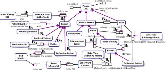
[Patient] arrives at [LaborWard] at [Date/Time] has Patient History (.id) Date/Time (.ddmmyy-hhmm) Delivering Patient B1 B2 B3 B4 B5 B6 B7 B8 B9 B10 B11 B12 B13 B14

Figure 6.ORM Scheme for the intrapartum process in Ugandan Hospitals

5.2 Decomposing the ORM Model

Conceptual schemes for realistic applications tend to be rather large, which makes them hard to handle for human modelers. By applying decomposition, a complex conceptual scheme can be split up in a set of smaller conceptual schemes that each, in turn, is easier to handle. Decomposing an ORM model takes a number of steps (see Section 4.2).

5.2.1 Separate Object Types with Their Roles Into Unique ORM Schemes

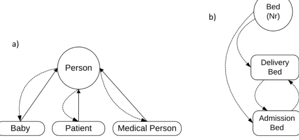
An ORM model is made up of different constructs and different relating object types made up of different objects playing roles. To apply the decomposition mechanism, object types are separated into different ORM schemes. In cases where the ORM model has supertypes (object types with unique properties), each supertype is represented with a hierarchy of substates like in Figure 6. Each supertype is represented separately. This helps the modeler to represent states for each ORM schema with a unique identifier although the objects in each state have similar properties. Using Figure 6 as a basis, we have supertypesBed andPerson. In the life of a person, we have three elementary states: being Baby, Patient andMedical person. In the life of a bed, we have two elementary states; Delivery Bed and Admission Bed. The ORM sub-scheme for object types Person and Bed are represented in Figure 7. Object type Bed, has four different transitions

B1,B2,B3,B4 5. For state admission bed (

A

), we have transitions (B1,B2)and for state delivery

bed (

_D

), we have transitions(B3,B4). So

A

=

B1,B2 and

D

=

B3,B4 .

Explanation: Initially, the bed is empty (B1), when a patient is admitted, she occupies the empty

bed (B2). During delivery time the patient occupies the delivery bed (B4) (in this case one patient

occupies two beds the admission bed and delivery bed). The delivery bed is initially empty but when a patient is ready for delivery she occupies this delivery bed for a period of time before and after she is taken back to her admission bed (B2), see the arrows between (B1), (B2), and (B3), (B4).

In the running case study, the hospital(s) have limited resources, e.g. beds, medical personnel etc. Therefore a patient does not have the luxury of not occupying a bed when allocated one due to constrained resources. Note that in Figure 8, we do not distinguish between allocation of a patient to a bed and actual occupancy of a bed by a patient.

5.2.2 Handle Each Object Type Independently

In order to improve conceptualization of the SFD model, handle each object type independently.

Person

Baby Patient Medical Person

   

Bed (Nr)

Delivery Bed

Admission Bed

  a) 

b)

Figure 7.ORM sub-scheme for object types Person (a) and Bed(b)

Bed

B2

B1

B4

B3

Admission Bed

Delivery Bed

 

Figure 8.ORM sub-scheme for object type Bed

Doing so enables a modeler to understand how objects in each state relate to one another. For each object type;

1. Give each role a unique identification.

2. Categorize states into elementary and compound states. 3. Represent states in order of activity occurrence.

4. Add directed paths.

Once the modeler understands the states and state transitions in each object type or hierarchy, (s)he is able to analyze the model behavior at a conceptual level.

Example 1. When a patient arrives at the hospital, the nurse on duty records her details (Patient

His-tory). Here the state Patient History is initiated, it can only be updated when that patient next visits the hospital (see Figure 9). Patient History has two transitions ‘is initiated’ and ‘record’.

 

Figure 9.ORM sub-scheme for object type Patient History

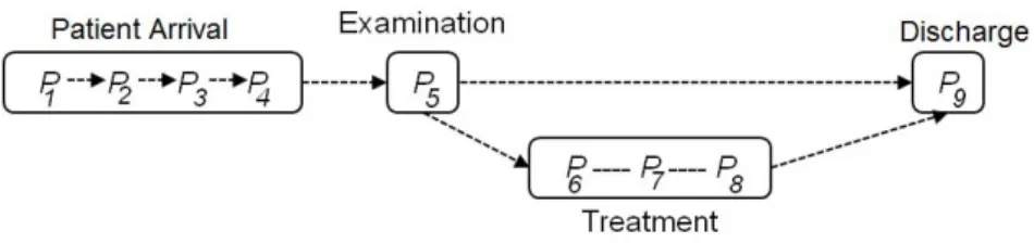
Patient: At a higher level of abstraction the patient intrapartum starts with Patient Arrival. Then the patient is examined, leading to eitherTreatment or (if no treatment is required)Discharge. After treatment, the patient is discharged. In Figure 10 we can see this main structure, but the figure also displays the further details of the compound states.

Figure 10.Detailed patient Intrapartum model

Explanation: When the patient arrives at the hospital, she queues up (P1) then she is registered (P2) by

the nurse, after registration patient history is updated (P3). We have:

A

=

P1,P2,P3,P4 ,

X

=

P5 ,

T

=P6,P7,P8 and

D

=

P9 .

After recording patient history, the patient waits to be examined (P4). When her turn comes she

is examined (P5), depending on the findings, she is either admitted (P6) or discharged (P9). If she is

admitted (P6), she is monitored (P7) every 30 minutes until she gives birth (P8). After giving birth she

is discharged (P9).

Medical Person(s) sub-states: The state Medical Person, has two base states Nursesand

Obstetri-cians. These states are contained in four different complementary statesMedical Records (

_M

),

Exami-nation (

_X

),Treatment (

_T

)andDischarge (

_D

)(see Figure 11). Some of these states are similar with the

obstetrician’s state. This is because in a hospital, if a case is very sensitive, for instance, an operation, it is handled by an expert who in this case is the obstetrician.

Figure 11.Nurse state model

Explanation: The life model of a Nursehas the following states; Administrates (A1), Monitors (A2),

Examines (A3), Admits (A4), Records History (A5), Establishes Dilation Stage (A6), Births Baby (A7)

and Discharges (A8). The life model of anObstetricianhas four states; Examines ( ¯A3), Admits ( ¯A4),

Birth Baby ( ¯A7) and Discharges ( ¯A8). These states are contained in three different complementary states

Examination,TreatmentandDischarge. In Figure 11 and Figure 12 we present the life model of a nurse

and an obstetrician respectively. We have

_P

=A1,A5 ,

X

=

A3,A6,A4,A¯3,A¯4 ,

T

=

A2,A7,A¯7

and

_D

=A8,A¯8 .  

 

 

 

5.2.3 Merge Different Decomposition Levels and Represent Them as a Whole

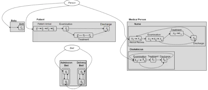
Having handled each object type or hierarchy independently it is important that the different ORM schemas are merged into one complete model. In Figure 13, we represent all the decomposition levels in the ORM schemes.

Figure 13.Decomposition levels in the ORM scheme shown in Figure 6

In this merged model, all the decomposition levels can be viewed. Understanding the state changes help the modeler define SD influencing transitions and input parameters. These influenc-ing transitions and input parameters are discussed in Subsections 4.1. After this step, SFD input parameters or values are easy to define because all existing states and transitions are already iden-tified.

6

Simulation

In this section, we discuss how an extended ORM scheme is converted into a stock and flow diagram. The ORM extensions we introduced, add essential System Dynamics concepts to the conceptual level description of ORM. As a result, the conversion is rather straightforward. This conversion focuses only on the states of object types and their transitions. The decomposition structure is ignored, since System Dynamics has no decomposition mechanism.

To construct the stock and flow model in Figure 14, we used the STELLA software pack-age [56]. This packpack-age provides a practical way to dynamically visualize and communicate how complex systems really work; and to derive simulations. It, for instance, allows simulation ‘run’ systems over time, sensitivity analysis which reveals key leverage points and optimal conditions and partial model simulations which allows focus analysis on specific sectors or modules of the model. Results from the SFD are then presented as simulation in graph or table form. STELLA contains some aggregation operators like SUM, MIN, MAX etc. to combine values of two or more quantities. To enable simulation, mathematical equations for all model variables were de-fined thereby specifying the behavior of each model variable with exactly one equation. These equations depicted how defined variables change over time.

From the merged model in Figure 13, we have the following main decomposition levels: “Baby”, “Patient”, “Medical Person”, “Delivery Beds” and “Admission Beds”. 6 _The

decompo-sition levels in Figure 14 are depicted as stocks and in each there exists states and trandecompo-sitions i.e:

• “Patient Arrival”:

_A

=P1,P2,P3,P4

6_{To minimize on the complexity of the model, the Bed decomposition level and a number of transitions}

• “Patient Examination”:

X

=P5,A3,A6,A4,A¯3,A¯4 • “Treatment”:

_T

=P6,P7,P8,A2,A7,A¯7

• “Discharge”:

_D

=P9,

• “Medical Records”:

_M

=A1,A5

These states are categorized into flows and converters depending on the definitions stated in Sec-tion 3.2. For each decomposiSec-tion level presented in Figure 13, we identified flows, i.e. inflow “Births” for stock “Babies”, and inflow “Patient examination” and outflow “Discharges” for stock “Patients”. The remaining states and some transitions are represented as converters (auxiliary vari-ables). These were added because they influence the behavior of the quantities in stocks through flows. The equations defining the stock quantities are placed in the converters and flows. 

       

   

SFD 1: Patient Life Stock and Flow Diagram representation     

  Graph 1: Simulation Results for Stocks Birth, Medical Person and 

Patients 

  Graph 2: Simulation results for flows Discharge, Births and  Examined 

patients   

 

 

Babies

Patients

Medical Persons

Patient examination

Discharges Treatment

Examination duration

medical Records Patient

Arriv als

Births Dilation

Examination

Capacity Medical persons on duty

Figure 14.An SFD and resulting Simulations for a patient life model

In SFD 1, depicted in Figure 14, we see the stocks (“Patients”, “Babies” and “Medical Per-sons”), the auxiliary variables (“Dilation”, “Treatment”, “Patient arrivals”, “Medical records”, “Examination duration”, “Examination capacity” and “Medical persons on duty”) and the flows (“Patient examination”, “Births” and “Discharges”)

Inflows and outflows are rate variables with dynamic values, .i.e. they change over time. The behavior of flows is specified by the rate equation. In Figure 14, there are two inflows (“Patient examination” and “Births”) and one outflow (“Discharge”). The equation for inflow “Patient ex-amination” is built upon two auxiliary variables “Patient arrival” and “Examination duration”. The equation for inflow “Births” is built upon one auxiliary variable “Dilation”, one inflow “Patient ex-amination” and one stock “Medical persons”. The equation for outflow “Discharge” is built upon one inflow “Births” and two auxiliary variables “Medical persons on duty” and “Treatment”. The rate variables assigned to outflow “Discharge” control the decrease of stock “Patients”.