DESIGN AND VALIDATION OF A MICROFLUIDIC DEVICE FOR CONTROLLED CELL STIMULATION
Stewart Monnich Peters
A thesis submitted to the faculty of the University of North Carolina at Chapel Hill in partial fulfillment of the requirements for the degree of Master of Science in the Department of Biomedical Engineering (School of Medicine)
Chapel Hill 2008
Approved by:
© 2008
ABSTRACT
Stewart Monnich Peters:
Design and Validation of a Microfluidic Device for Controlled Cell Stimulation (Under the direction of Shawn Gomez and Glenn Walker)
Understanding how cells receive chemical signals from their surrounding environment and transform them into appropriate responses is a fundamental problem in biology. A
ACKNOWLEDGEMENT
I would like to thank my advisors, Dr. Shawn Gomez and Dr. Glenn Walker, and third committee member, Dr. Oleg Favorov, for their help and advice throughout the course of this research.
TABLE OF CONTENTS
LIST OF TABLES ... vii
LIST OF FIGURES... viii
CHAPTERS
1.
INTRODUCTION... 11.1 Background... 1
1.1.1 Cell Signaling... 2
1.1.2 Previous Work... 3
1.2 Cell Simulation Theory... 5
1.2.1 Flow Theory ... 6
1.3 Problem Statement ... 9
2.
MATERIALS AND METHODS ... 122.1 Device Design... 12
2.1.1 Initial Design Concept... 12
2.1.2 Final Device Design ... 13
2.2 Device Fabrication... 16
2.2.1 Micromolding Overview ... 16
2.2.2 Fabrication Challenges ... 16
2.2.3 Final Fabrication Process ... 19
2.3 Experimental Process... 22
2.3.1 Characterization... 22
2.3.2 Experimental Validation... 23
3.
RESULTS AND DISCUSSION ... 263.1 Plug Flow Characterization... 26
3.1.1 Image Processing... 27
3.1.2 Theoretical Assumptions... 29
3.1.3 Characterization Results... 30
3.2 Biological Test / Validation ... 33
3.2.1 HEK Ethanol Exposure ... 33
4.
CONCLUSION ... 384.1 Project Synopsis... 38
4.2 Design Improvements ... 39
4.3 Future Implications ... 41
APPENDIX A: Fabrication and Operations Manual... 42
LIST OF TABLES
Table 1. Fluid Inputs ... 14
Table 2. Device Operation - only one valve-set open at a time... 14
Table 3. Fabrication Bonding Techniques Evaluation... 19
LIST OF FIGURES
Figure 1. Cell as an input-output system... 5
Figure 2. Plug moving over cells from left to right ... 6
Figure 3. Parabolic Dispersion of Plug ... 7
Figure 4. Taylor dispersion acting on a plug... 7
Figure 5. Plug after equilibrated over cross-section of channel and taken Gaussian profile ... 7
Figure 6. Plug spreading compared to original square profile ... 9
Figure 7. Plug profiles observed from a fixed point... 9
Figure 8. Initial 2-layer design with monolithic valves: top-down view... 12
Figure 9. Diagram of loading reagent into main channel and flowing plug downstream ... 13
Figure 10. Device Design - Main channels in black, Valve Control channels colored RGB... 14
Figure 11. Fluid flow in device with valves sets B and C closed ... 14
Figure 12. Equivalent electrical circuit model of microfluidic device with only Valve B open. ... 15
Figure 13. Custom Valve-Control Syringe Holder... 15
Figure 14. Overview of fabrication process... 16
Figure 15. Two layers not bonded and shifted when removed ... 17
Figure 16. Fluoropolymer transparency film method introduced bubbles that destroyed membrane ... 18
Figure 17. Main channel collapsed... 18
Figure 18. A. Bottom layer B. Top layer... 19
Figure 19. Valves leaking with square side walls ... 20
Figure 20. Composite master with SU-8 2025 positive photoresist rectangular structures and SPR 220-7 reflowed positive photoresist inserted into valve areas... 21
Figure 21. Hydraulic valve control channel forces membrane downward collapsing main channel below. Square channel geometries do not close completely and leak. The valve areas require rounded geometries... 21
Figure 22. Bottom-layer masks. A. Negative photoresist mask B. Positive photoresist mask... 21
Figure 24. Plug loading and delivery (A) Plug loaded into main channel (B) Plug leaving loading area, flowing downstream (C) Plug once it has reached cell-seeding area where it
is imaged... 27
Figure 25. Extracting percent of light transmission. A. Baseline - channel empty B. Plug centered in view C. Percent of light transmission ... 27
Figure 26. Food coloring concentration vs. percent of light absorbance... 28
Figure 27. Fluorescein plug images – red line shows values used to calculate intensity ... 29
Figure 28. Plug concentration profile centered in seeding area... 30
Figure 29. Plug concentration versus time centered in seeding area ... 32
Figure 30. Sample fluorescence images taken after live-dead assay. Live cells are shown in green. (A) Control (B) 40s exposure (C) 2.5 min exposure (D) 5min exposure (E) 8min (F) 12.5min exposure... 34
Figure 31. Ethanol plug exposure profiles in time... 35
Chapter 1
INTRODUCTION
1.1 Background
Biomedical engineering is the application of engineering principles and techniques to the medical field, combining the design and problem solving skills of engineering with medical and biological sciences. The human body is arguably the most advanced system on the planet. There are many physiological systems within the body which operate in concert with one another to maintain life and complex functionality, but due to this complexity when something is not functioning properly in the body it can be difficult to properly diagnose or treat. The challenges faced are far from trivial, but as the understanding of these biological systems is increased through research, the capabilities of patient health care and the quality of life of individuals will continue to improve.
1.1.1 Cell Signaling
All organisms must respond to their environment to survive. Within a multicellular organism, cells need to be able to communicate with one another in complex ways if they are to be able to govern their own behavior for the benefit of the organism as a whole. Even unicellular organisms, such as yeast cells, need to communicate with other cells to initiate mating. Through studying yeast cells, many proteins have been identified that are required in the signaling process including cell-surface receptor proteins, GTP-binding proteins and protein kinases [2]. Typically, initiation of cell signaling begins when extracellular signaling molecules bind and activate protein receptors on the cell surface.
Cells are enclosed in bi-lipid plasma membrane that separates the inside of the cell from the extracellular fluid. Cytosol is a saline solution present inside the cell. Signaling molecules may be secreted into the extracellular space by a signaling cell through exocytosis, diffuse through the plasma membrane, or be attached to the surface of the cell. Signaling molecules include proteins, amino acids, nucleotides, steroids, and dissolved gases. These molecules can travel through the interstitial fluid by diffusion over short distances or be carried through the bloodstream throughout the body, such as hormones secreted by endocrine cells. The majority of signaling molecules are hydrophilic and bind to transmembrane cell-surface receptors that relay the signal to the inside of the cell. Other molecules are sufficiently small and hydrophobic and can diffuse through the plasma membrane binding to receptor proteins within the cell. [2]
parts of the cell, amplify the signal, or pass the signal on to the next component in the chain eventually influencing the cell behavior such as movement, metabolism and gene expression. [2]
Cell function and behavior is tightly controlled through feedback mechanisms and a target cell’s response may be abrupt or long lasting. Signal molecules are regulated by the cells and can have short half-lives. The duration and concentrations of these signaling molecules are critical in the response of a target cell. Some cells exhibit nearly an all-or-none response based on whether or not a threshold concentration is reached for a specific molecule. Many other cellular responses are proportional to the concentration, although desensitization may occur over time to prolonged stimulation. [2]
1.1.2 Previous Work
Complete washing in standard wells is difficult and usually requires multiple rinses. Microfluidic devices have been shown to have improved sample treatment and washing over standard wells [11]. This is due to the fact that microfluidic devices operate with constant fluid perfusion. In perfusion culture, steady state concentrations of nutrients and metabolites can be achieved. Also when a toxicant or other chemical stimuli is added to the medium, it is
administered to the cells at a defined constant concentration [12]. Microfluidic devices promise to enhance fundamental biological research by offering more consistent and precise experimental conditions than multi-well plates. Microfluidic devices have already been used for cell sampling, cell trapping and sorting, cell treatment, and cell analysis [13].
1.2 Cell Simulation Theory
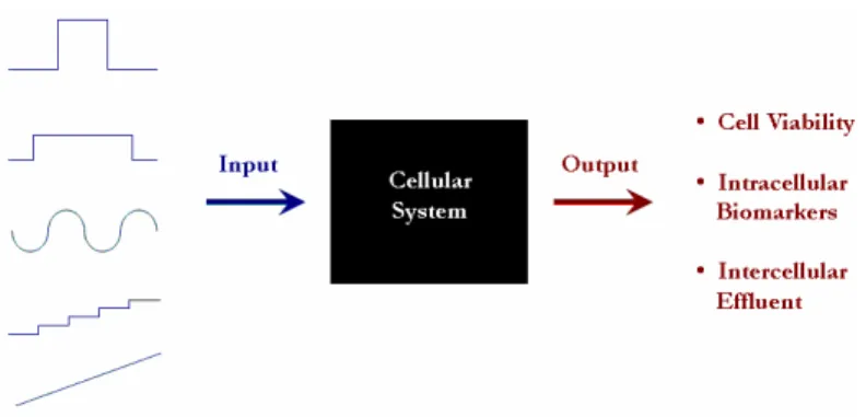
As just discussed, the use of microfluidic technologies provides the opportunity to establish a highly controlled environment in which to study cell signaling, and more precisely control the stimulation of cells. In particular, the ability to deliver reagents in discrete packets to cells with high spatiotemporal precision will greatly benefit the quantitative study of cellular signaling processes. In some scenarios, the reagent plug is analogous to an input signal for a “black-box” system. The output signal is embodied by the cellular response to the input signal. By probing cellular systems with a variety of input signals, a more complete picture of their behavior will emerge, leading to an increased understanding of many cell types. Figure 1, illustrates this concept of the cell as an input-output system.
Figure 1. Cell as an input-output system
cellular signaling information, the possibility arises to employ well-established computational approaches in the modeling and simulation of these systems. Long-term this information could further medical advancements, for instance it could reveal ways to disrupt the process in which cancer cells successfully metastasize elsewhere in the body.
1.2.1 Flow Theory
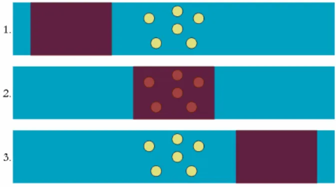
Microfluidic devices are primarily an arrangement of enclosed channels capable of
manipulating fluid on the sub-millimeter scale. Figure 2 illustrates a chemical stimulus packet, or plug, moving past cells within the channel. Again, these applied chemical signals are chosen so as to stimulate cell-membrane receptors and evoke a particular signaling response.
Figure 2. Plug moving over cells from left to right
Figure 3. Parabolic Dispersion of Plug
Diffusion acts to mix the concentration differences in the cross section of the channel across the width and along the length of the plug as well. Taylor dispersion is the combined effect of convection and diffusion, and although the plug is well defined at first, Taylor dispersion alters the shape of the plug as it flows down the channel. Figure 4, illustrates plug shape
dispersion with diffusion forces represented by the arrows extending in all directions.
Figure 4. Taylor dispersion acting on a plug
Although, spreading due to diffusion and convective transport change the shape of a plug flowing through a channel, Taylor showed that any finite cloud of solute eventually becomes uniformly spread out over the cross-section of the flow and takes up a Gaussian profile in the direction of flow [18]. The characteristic time for convective transport is the distance the plug travels divided by the flow velocity [19]. The mean plug flow velocity, u, (mm/s) can be calculated from the volumetric flow rate (µL/min), v, and the dimensions of the channel, height h and width w, as shown in Equation 1.
60 * w * h
ν
υ
= (1)The time scale for the plug to diffuse across the width of the channel, w, is on the order of O(w2/D), for a solute with diffusion coefficient, D [20]. This is when the solute has equilibrated over the cross-section of the channel, after which time the concentration profile can be
represented by a one-dimensional Gaussian profile in the direction of flow, as represented in Figure 5.
Several variables are required to calculate the concentration profile. The Peclet number is a ratio of the rate of advection to diffusion. Advection, or convection, affects how the plug is skewed based on velocity, and diffusion affects how fast the solute spreads in all directions in time. As shown in Equation 2, the Peclet number, Pe, is based on the characteristic length, L, which corresponds to the smallest dimension of the channel, the flow velocity, u, and the diffusion coefficient of the solute, D. Shown in Equation 3, the long-time effective dispersivity, Deff, can be calculated to account for both diffusion and convection. The effective dispersivity is based on Pe, D, and the constant k based on the geometric shape of the channel. For example, a rectangular channel with aspect ratio, w/h, of 10, the constant k is 33/560 [19].
D L
Pe=
υ
(2)D
eff=
D
(
1
+
kPe
2)
(3)The final factor that affects the profile is the initial plug length, p. The relative concentration of the solute at position, x, in a channel for time, t, can be calculated from the diffusion equation using Deff. Equation 4 gives the solution for the one-dimensional concentration profile centered at position at u*t [21].
+ − + − − = t D t x p erf t D t x p erf C t x C eff
eff 2 *
) * ( 2 * 2 ) * ( 2 2 1 ) , ( 0
υ
υ
(4)The position of the plug in time and its spreading due to Taylor dispersion can be calculated based on the flow velocity and diffusion coefficient. Equation 4 provides the
concentration at a specific position in a channel for a specific time. Therefore the concentration can be plotted with respect to time or position. For example, if you were riding on top of the plug, the profile would be a symmetrical Gaussian curve at any given time. If you were an observer sitting beside a channel measuring the concentration as the plug moved by, the
Consider a channel 10µm tall and 100µm wide with a plug 1mm long, with D of 0.001mm2/s, which you send down the channel at different flow rates. If you rode on the plug and took a snapshot once you had traveled 5 mm you would see the profiles in Figure 6. The red curve shows the initial shape of the plug.
Figure 6. Plug spreading compared to original square profile
If for the same plugs, instead of riding them you watched the plug move by through a window 5 mm down the channel you would see the concentration profiles shown in Figure 7.
Figure 7. Plug profiles observed from a fixed point
1.3 Problem Statement
allow cellular response to be studied at an unprecedented level of detail. In this scenario, the reagent plug is analogous to an input signal for a cellular system. The amplitude of the stimulus signal is controlled by the concentration of the chemical, while the time duration is controlled through the width of the plug and the flow rate. The output response of the system is
characterized by the resulting changes in measured intracellular and extracellular behavior. By probing cellular systems with input signals of varying complexity, along with measuring the output response at many points within the signaling network, we expect to obtain a more complete picture of cellular function and dysfunction.
Investigating cell signaling includes cell stimulation, response measurement and data analysis. The first place to start and weakest aspect in existing methodologies is in controlled cell stimulation. The goal of this research was to create a device that would show proof-of-concept for the controlled stimulation of cells that could further the effort in researching cell signaling. The main goals of this research included: 1) develop a microfluidic device that can deliver a pulse stimulus to cells in a highly controlled manner; 2) characterize the stimulus dose administered to the cells; 3) and validate the device design by exposing cells to a toxicant plug and measuring cell viability.
We have developed a microfluidic device that can deliver chemical treatments to cells with high temporal resolution while simultaneously allowing the ability to quantitatively measure the cellular response. The main structure of the device is made from multiple layers of
The plug flow profile has been characterized by imaging plugs within the microchannel as they flowed past the cell-seeding area. Plug profiles were evaluated in brightfield and
Chapter 2
MATERIALS AND METHODS
2.1 Device Design
2.1.1 Initial Design Concept
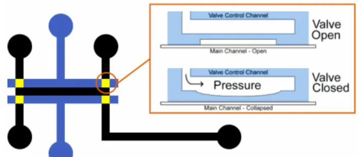
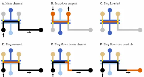
The purpose of the microfluidic device to be developed was to have a device that could deliver a pulse stimulus to cells in a controlled manner. This could be achieved by flowing a plug of chemical reagent over cells seeded within a channel. A system of valves is required to load the plug into the main channel, as shown in Figure 8. This was to be achieved by incorporating monolithic microfabricated valves into the device [22], which simply means the valves are an inherently built into the device based on the fabrication process.
Figure 8. Initial 2-layer design with monolithic valves: top-down view
below it. Using this system of valves, a reagent can be inserted into the main channel, and then the plug can be sent downstream as illustrated in Figure 9.
Figure 9. Diagram of loading reagent into main channel and flowing plug downstream
Figure 9A shows fluid flow in the main channel. Using the valves shown in 9B and 9C, flow can be directed from a separate input to fill a section of the main channel with a reagent. Then when the valves are manipulated to allow flow through the main channel again, the plug is moved downstream through convective transport with the flow through the main channel. Initially the plug has a square 100% concentration profile, but Taylor dispersion alters the shape of the plug into a Gaussian profile as it flows down the channel.
2.1.2 Final Device Design
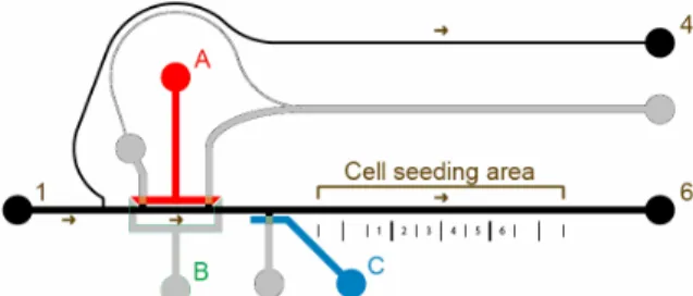
control the flow of fluid into the device. Valves exist where two channels overlap. The hydraulic valves are open by default due to the elasticity of the membrane and close when pressure is applied, forcing the membrane downward to seal the channel below.
Figure 10. Device Design - Main channels in black, Valve Control channels colored RGB.
Table 1. Fluid Inputs Table 2. Device Operation - only one valve-set open at a time
When valve-sets A and C are closed, there are the only two parallel paths for the fluid to flow through, shown in Figure 11.
Figure 11. Fluid flow in device with valves sets B and C closed
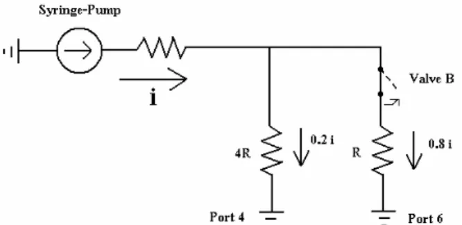
The channel dimensions (height - h, width - w, length - L) for the drain line that leads to port hole 4 correspond to four times the relative resistance of the main channel path to port hole 6, based on the resistance equation for a channel of a rectangular cross-section [23] shown in Equation 5.
1 1
192
12µL h ∞ nπw−
Port Input
1 Cell Medium 2 Reagent / Stimulus 3 Cells
Step Input Open Valve(s)
1. Seed cells C
2. Perfuse cells with cell medium B
3. Load reagent plug A
An equivalent electrical circuit can be made for the microfluidic device, representing fluid flow as current, i, shown in Figure 12. Based on Ohm’s Law, when only valve-set B is open, 80% of the fluid flows through the main channel to port 6 and 20% flows through the drain to port 4.
Figure 12. Equivalent electrical circuit model of microfluidic device with only Valve B open.
When valve-set B is closed (equivalent electrical model is open switch), 100% of the flow from the syringe pump flows to port 4, since it is the only path available. Typical flow rates used range from 0.005µL/min to 0.1µL/min, which translates to flow velocities in the main channel of 0.007mm/s to 0.148mm/s. It is necessary to have the drain line so that pressure does not build when valve-set B is closed. In order to have 100% of the flow from the syringe pump sending the plug down the main channel, a valve would have to be added to block the drain line and an electrically controlled valve system would have to be implemented to provide
instantaneous opening of the main valve and closure of the drain valve. We did not have such a sophisticated control and used a custom syringe holder to hold a syringe in a compressed state to maintain pressure on the valve, shown in Figure 13.
2.2 Device Fabrication
2.2.1 Micromolding Overview
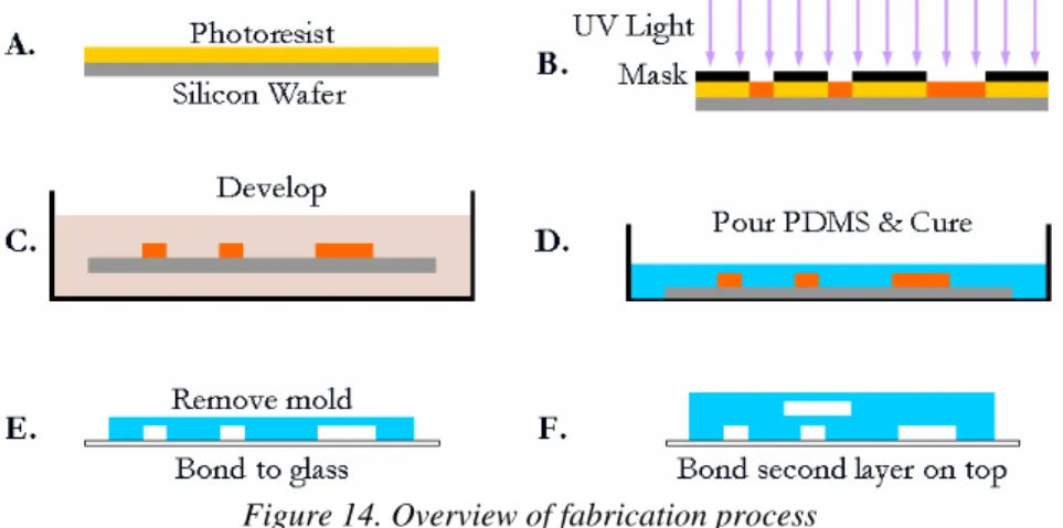
Microfluidic devices are made using rapid-prototyping techniques incorporating photolithography and micromolding. A mold, called a master, is created for each layer of a device, and PDMS is poured over the mold then cured to cast the channel features desired. The PDMS cast creates the top and sides of the channels and is bonded to glass for the bottom surface. This process is outlined in Figure 14.
Figure 14. Overview of fabrication process
First a mask is made from the design to selectively block UV light. Photoresist is sensitive to UV light and chemically changes when exposed to it, making the exposed areas more or less
susceptible to development depending on the type of photoresist. Development removes the portions of photoresist not wanted leaving the master, or mold from which devices can be made. PDMS devices can be cast from the mold. Port holes can be punched out with a hollow needle. Then PDMS layers can be bonded to glass or other PDMS layers.
2.2.2 Fabrication Challenges
aligned over one another. The device design was modified to make this process as easy as it could be throughout the development process, although the fabrication process proved a significant challenge. The membrane had to be robust and isolate the two layers but also be flexible. The PDMS layers also had to be bonded sufficiently to withstand the pressure required to deform the membrane to collapse the roof of the lower channel with pressure applied. These valves also had to operate reliably, seal completely and remain closed, or the stimulus dose would not be controlled.
We investigated several methods to create the membrane and bond the two layers. In the article by Unger et al, the process for creating these valves was described using a PDMS product from GE [22]. PDMS is created by mixing a base with a curing agent that covalently bond, curing in a certain amount of time based on the temperature. The base and curing agent are normally mixed in a 10:1 ratio. To promote bonding of the two PDMS layers, Unger used a 30:1 ratio on the top layer and a 3:1 ratio for the lower layer. Both layers were half-cured, then placed together and fully cured to ensure a solid bond. We use a different PDMS product from Dow Corning and were unable to get this method to work. On first attempt, the thin film would not peel up and destroyed the master. On a second attempt, the two layers did not bond sufficiently and could peel apart as shown in Figure 15.
Figure 15. Two layers not bonded and shifted when removed
apparent that a thin PDMS film ~ 50µm thick is far too thin to handle. Then we attempted to use a fluoropolymer transparency film to bond to the top of the membrane to add rigidity to the structure. After plasma treatment PDMS has a higher affinity to glass than the transparency. The bottom layer was bonded to glass and then the transparency was peeled off. Unfortunately bubbles that were in between the transparency and membrane destroyed the thin film, as shown in Figure 16.
Figure 16. Fluoropolymer transparency film method introduced bubbles that destroyed membrane
A final method was evaluated leaving the membrane on the wafer and plasma treating the membrane and top layer. Then the membrane was coated with methanol to allow precise
alignment of the layers and then they were heated evaporating the methanol and bonding the layers together. Then both layers were peeled off the master together and bonded to glass. In this method the two layers bonded together well, but the main channel collapsed when bonded to glass, shown in Figure 17.
Each method presented different challenges. It became apparent that the one of the methods would need to be perfected. After two attempts were made using each process, we evaluated each method based on the criteria shown in Table 3.
Table 3. Fabrication Bonding Techniques Evaluation
Method Pros Cons
Alternative ratios and half-curing Proven method based on article May require purchasing different
PDMS Half-cure method w/ normal
ratios
PDMS easier to work with than alternative ratios
Worst bonding based on initial trials
Transparency transfer of membrane to glass
Showed promise and bubbles could be prevented by careful application of transparency
Would need to bore port holes through PDMS and transparency
Plasma treatment and methanol alignment
Successfully bonded two PDMS layers on second attempt
Required cutting master to fit in plasma cleaner - risk shattering
With enough work, all of the methods were feasible, but we found that the
plasma/methanol procedure showed the most promise and we focused our efforts perfecting that method. Other challenges were encountered and the approaches for addressing these are described in more detail in the appendix. Eventually we developed a reliable process for fabricating the device with the monolithic valves for plug formation and delivery.
2.2.3 Final Fabrication Process
The multi-layer microfluidic device was fabricated by replica molding the two-part silicone elastomer (SYLGARD 184 Silicone Elastomer Kit, Dow Corning, Midland, MI)
polydimethylsiloxane (PDMS). Two masters were used to create the final multi-layer device, one for the bottom layer (main fluid channels) and another for the top layer (valve control channels). The designs for each layer are shown in Figure 18.
The final device consists of two PDMS channel networks separated by a thin PDMS membrane. Valves exist where channels in the top layer cross over channels on the bottom. The top layer master was created by spin coating negative tone photoresist (SU-8 2025, Microchem Corp., Newton, MA) on a silicon wafer. After a soft bake on a hot plate, the photoresist was selectively exposed with ultraviolet light for 50s (BlakRay B-100A, UVP, Upland, CA) through a high-resolution transparency containing the channel design.
These photolithography techniques typically create channels with vertical walls, so that the channels have rectangular cross sections. However, preliminary experiments indicated that the valves were not sealing properly, leaking on the sides of the valves, presumably because of their rectangular cross sections, as shown in Figure 19.
Figure 19. Valves leaking with square side walls
Figure 20. Composite master with SU-8 2025 positive photoresist rectangular structures and SPR 220-7 reflowed positive photoresist inserted into valve areas
Figure 21. Hydraulic valve control channel forces membrane downward collapsing main channel below. Square channel geometries do not close completely and leak. The valve areas require rounded geometries.
First, the majority of the mold was created by spin coating negative tone photoresist (SU-8 2025, Microchem Corp., Newton, MA) at 2.5k rpm for 30s on a silicon wafer to create a 30µm high coat. The negative photoresist was selectively exposed for 45s with UV light through a transparency mask containing the design, shown in Figure 22A.
Figure 22. Bottom-layer masks. A. Negative photoresist mask B. Positive photoresist mask
CA) through a high-resolution transparency mask, shown in Figure 22B. The master was allowed to sit for 2 h before development to allow the chemical change from the UV light to fully set in. After development, to create rounded channels the master was slowly ramped to 115 °C to prevent bubble formation and held there for 20 min to allow the positive resist to reflow.
To create the bottom layer and membrane, PDMS was poured over the bottom master and spun at 1000 RPM and then cured at 95 °C for 80 min to create a 60 µm thick coat from the Si wafer. The top layer was cast off the first master as a PDMS slab of arbitrary thickness. The top layer PDMS slab and bottom layer PDMS membrane, still on the wafer, were covalently bonded together using an oxygen plasma treatment. The PDMS layers were plasma treated and aligned under a stereoscope with methanol and then baked on a hot plate at 85°C for 60 min to evaporate the methanol. Weights totaling twenty pounds were placed on top of the stacked PDMS layers to manually force out any vapor bubbles that had formed between the two layers and ensure
complete bonding.
Once the two layers were bonded, they were peeled off the bottom layer master, cut into the desired shape and port holes were cored out with a blunt 16 gauge needle. The PDMS two-layer device was then bonded to a glass slide using plasma treatment. Flow was introduced into the microfluidic device via Tygon tubing (Cole-Parmer, Vernon Hills, IL) with dimensions of 0.51 mm I.D. x 1.52 mm O.D. The tubing was inserted into the PDMS port holes and connected to a syringe pump (Pump 11 Pico Plus, Harvard Apparatus) via syringes fitted with blunt 25 gauge dispensing needles (Howard Electronic Instruments, El Dorado, KS).
2.3 Experimental Process
2.3.1 Characterization
(Olympus IX71). Each brightfield image was captured using IPLab (Scanalytics, Rockville, MD) at an exposure time of 1 ms with the plug centered in the cell-seeding area, shown in Figure 10, for a range of flow rates. These images were manipulated using Matlab (Mathworks, Natick, MA) code that we developed to derive the concentration profile of the plug. A baseline image was taken before each plug arrived, which was used to calculate the percent of light transmission of the plug image. Then according to Beer’s Law, the percent of absorption was calculated which is linearly proportional to the percent of dye concentration to create a plot for the plug
concentration profile across the field of view.
Fluorescein (Acros Organics) was used to fluorescently quantify the concentration of the plug by dissolving it in acetone at a concentration of 10 mg/mL and then diluting it in DI water to 0.1mg/mL. Fluorescence images were acquired with a FITC cube (Chroma Technology,
Brattleboro, VT) and the Hamamatsu camera and Olympus microscope. Time series images were captured using IPLab with 150ms exposure times as the plug moved past the cell-seeding area, shown in Figure 10, for a range of flow rates. For each image, fluorescence intensity was averaged on a slice of an image centered in the seeding area, 104 pixels high and 4 pixels wide, which was scaled based on the initial intensity to create concentration versus time plots.
2.3.2 Experimental Validation
and B were closed. The channel between port 3 and 6 was then exposed to a Type I collagen solution (4.8 µl of 3.13 mg/ml Type I rat tail collagen, 1.0 µl of 2.0 N acetic acid, and 49.0 µl sterile water) for 1 h to promote cell adhesion. After exposure to collagen, the microchannels were flushed with PBS and then HEK cell medium (Clonetics KGM-2, Cambrex Corp.).
Twice passaged and cryopreserved normal neonatal human epidermal keratinocytes (NHEK) (Clonetics NHEK, Lonza Bioscience) were thawed in a 37°C water bath, suspended in 12 ml of cell medium, and centrifuged at 1000 rpm for 5 min. After aspirating the medium, the cells were resuspended to a concentration of 1,000 cells per microliter. HEK were seeded in the device between port 3 and 6 at flow rate of 0.20 µl/min. The device was then placed in the incubator at 37°C and 5% CO2 for 1-4hrs before running the ethanol plug. While in the incubator, the cells were perfused with medium at a flow rate of 0.15 µl/min.
The reagent was a mix of 30% ethanol, 50% PBS, and 20% food coloring by volume. The food coloring was present to verify the plug loaded properly and allowed visual confirmation that the valves were not leaking ethanol into the main channel. The syringe pump was set to the volumetric flow rate corresponding to the desired flow velocity in the main channel. The valve system was used to fill the reagent loading area with the 30% ethanol solution and then the plug was flowed past the cells at the desired flow rate. Once the plug reached port hole 6, the well was dried to prevent ethanol from diffusing back into the channel. The flow rate was set to 0.20
µl/min and the device was returned to the incubator for 15 minutes before the live-dead assay was introduced.
Chapter 3
RESULTS AND DISCUSSION
3.1 Plug Flow Characterization
To characterize the plug concentration profile changes due to Taylor dispersion we imaged dye plugs as they reached the cell-seeding area. Dye images can be taken in brightfield or fluorescence microscopy. In brightfield, food coloring dye is a good choice, although some calculations are necessary to determine the concentration from the percent of light transmission. Fluorescein is a fluorescent dye whose intensity is directly proportional to its concentration. Unfortunately, it was too dim to image the entire plug and the mercury lamp is non-uniform which would be difficult to correct for across the full field of view. Rhodamine is another fluorescent dye that fluoresced more brightly than fluorescein, but proved problematic since it leeched into the PDMS. We tried to correct for this using parylene deposition, but the parylene did not coat the entire channel, just near the port holes. Figure 23 shows the PDMS fluorescing after Rhodamine has been flowed through the channel and rinsed, revealing where the parylene coating ended.
In order to image a plug centered in the cell-seeding area, the best method proved to be food coloring dye plugs. We used the device to send plugs at various flow rates and captured images of the plugs, as shown in Figure 24. Although fluorescein was too dim to image the entire plug with a 2x objective, using a 10x objective we were able to image the intensity of fluorescein at the center of the seeding-area to determine the concentration profile exposure at a stationary point through time series images.
Figure 24. Plug loading and delivery (A) Plug loaded into main channel (B) Plug leaving loading area, flowing downstream (C) Plug once it has reached cell-seeding area where it is imaged
3.1.1 Image Processing
Imaging food coloring dye plugs in brightfield enabled us to use an exposure time of just 1 ms with the plug centered in the cell-seeding area, preventing blurring. Then using a baseline image of the channel before the plug arrived, the percent of light transmission could be extracted, as shown in Figure 25. The data from these images were processed using Matlab code that we developed to derive the dye concentration at each pixel value. The one-dimensional plug profile was calculated from averaging each column of pixels across the width of the channel.
The percent of light transmission was calculated on a one-to-one pixel basis. The
intensity value for each pixel in the plug image was divided by the respective pixel in the baseline image, which also corrected for the non-uniformity of the light source. According to Beer’s Law, the concentration of a dye is linear with absorbance. The percent of absorption, A, can be
calculated from the percent of light transmission, LT, as shown in Equation 6. The percent of absorption is linearly proportional to the percent of dye concentration, and therefore the plug concentration profile can be calculated as shown in Equation 7. Concentration was calculated from the percent of light transmission of the plug, scaled by the percent of light transmission of the full concentration C0, from images of the plug in the loading area before dispersion.
(
%LT)
log-A
% = 10 (6)
(
)
(
0)
10 10 C of LT % log LT % log =
C (7)
At high concentrations of dyes light absorption may become non-linear. We measured the absorbance levels for food coloring and verified that there was a linear relationship with absorbance and concentration through 50% concentration, as shown in Figure 26.
Figure 26. Food coloring concentration vs. percent of light absorbance
proportional with light emission. Therefore the concentration was calculated by dividing the intensity values for each time point, by the fluorescence intensity of the plug before it was released.
Figure 27. Fluorescein plug images – red line shows values used to calculate intensity
3.1.2 Theoretical Assumptions
Initially the plug had a length of 3 mm with square 100% concentration profile. As previously explained in section 1.2.1, Taylor dispersion alters the shape of the plug as it flows down the channel. Eventually the solute becomes uniformly spread out over the cross-section of the flow and takes up a Gaussian profile in the direction of flow. At this point the concentration is uniform across the width of the channel and can be represented by a one-dimensional model calculated from Equation 4. Profile measurements should be made after the transient region once the plug has taken the Gaussian form, which limits the flow rates that can be used.
The upper flow velocity at which the plug should be fully diffused over the cross-section of the channel is O(L*D/w2) [20]. The length, L, between the center of the plug loading area and the cell-seeding area is 10.8 mm. The diffusion coefficient, D, for diluted food coloring dye in water is 5 x 10⁻⁴ mm2/s [24] and the channel width, w, is 300 µm. Therefore using food coloring in our device, the assumptions for Equation 4 are met at flow velocities under 0.06 mm/s, or volumetric flow rates under 0.041 µL/min on the syringe pump. Fluorescein has a higher diffusion
3.1.3 Characterization Results
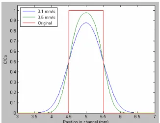
Plug flow profiles were characterized by imaging plugs within the microchannel as they flowed past the cell-seeding area. The plug is formed in the loading area at full, uniform concentration with a length of 3mm. As the plug travels down the channel, Taylor dispersion spreads the plug and morphs the initial square concentration profile into a Gaussian curve. Plug profiles were evaluated in brightfield and fluorescence microscopy by imaging the intensity of dye plugs and deriving their concentration profiles as previously explained. Food coloring plugs were imaged in brightfield centered in the cell-seeding area to derive the profile for the plug at an instant in time, using a 1 ms exposure time. Fluorescein plugs were imagined in time series images to provide concentration values at the center of cell-seeding area in time.
Qualitatively the plug profiles that were calculated from the experimental measurements of food coloring dye plugs correlate closely with the theoretical calculations. The measured and theoretical results for these experimental conditions show the general trend that dispersion is increased as the flow rate is decreased. Dispersion due to convective transport increases with increasing flow rates. Dispersion due to diffusion has the opposite effect, increasing with decreasing flow rates since it is time dependent and slower plugs take longer to reach the seeding area. These results confirm that diffusion is the dominating force for these conditions and provide confidence in the model.
The amplitudes for the measured results are lower than the theoretical, which may indicate that the plugs saw a higher effective dispersivity than expected. Regardless, the relative
differences amongst profiles for the measured and theoretical results are quite similar in terms of relative amplitude and spreading between the flow rates. It should be noted that the
one-dimensional model is a simplification of the system and therefore will yield differences no matter how precisely the parameters may correspond to the actual conditions.
Incidentally, there are factors that may contribute to an increase in effective dispersivity not included in the model. The valve system will affect the plug. Based on the footprint of the device, each valve has an active area of approximately 300 µm x 300 µm, each roughly 10% of the size of the plug. Opening of these valves will certainly disrupt the plug to some degree. The model also assumes that the plug has a constant flow velocity, while in reality it must accelerate which is not accounted for in the model. These results provide support that the model is a fair approximation for the system. However, the discrepancies also bring into question the system of measurement and the precision of Beer’s Law, that absorption is the negative log of light
transmission, for food coloring.
averaged together to create the intensity values which were scaled based on the initial
fluorescence intensity of the plug. The theoretical plot was created using D of 6.4 x 10⁻⁴ mm2/s, for fluorescein in water [25,26]. The plots are shown in Figure 29.
Figure 29. Plug concentration versus time centered in seeding area
previous works investigating Taylor dispersion on plugs of solute [18-20].
For experimental use, cells are stationary in the channel and the stimulus plug moves over them. The duration of the stimulus exposure is based on the flow rate and dispersion of the plug. It is the length of time it takes for the entire plug to move past the center of the cell-seeding area. Since the profile is asymptotic a more practical definition for the duration of exposure is the amount of time the concentration of the reagent is greater than 5% of C0 at the center of the cell-seeding area. The need for this definition and certain issues revealed through the characterization process expose limitations of this specific strategy of plug formation for stimulus delivery, which is discussed in the conclusion. However, these results show proof-of-concept and present a solid platform which can be built upon.
3.2 Biological Test / Validation
To validate that this device can be used for its intended purpose, we needed to conduct a biological test using cells. This confirmed that not only could we get cells into the device, but that we could stimulate them in a controlled manner. Proving the device was functioning as designed required using a test that would provide a predictable response. Therefore we decided to expose cells to toxicant plugs for a range of exposure times. We determined we would measure cell viability as the output. We hypothesized that cell viability would decrease with increased exposure time to a toxicant.
3.2.1 HEK Ethanol Exposure
However, cell viability versus time of exposure has not been studied and presents an appropriate validation test of the device.
The device was used to expose HEK cells seeded within the device to plugs of 30% ethanol by volume for a range of exposure times. A live-dead assay (calcein/EtH-D1 stain) was used to determine cell viability after the cells were exposed to an ethanol plug. As described in section 2.3.2, composite images were created using IPLab coloring live cells in green and dead cells in yellow or red. Live cells were counted and are indicated by exclusive fluorescence of calcein in green. Sample images are shown in Figure 30.
Figure 30. Sample fluorescence images taken after live-dead assay. Live cells are shown in green. (A) Control (B) 40s exposure (C) 2.5 min exposure (D) 5min exposure (E) 8min (F) 12.5min exposure
Figure 31. Ethanol plug exposure profiles in time
The live and dead cells were counted in the cell-seeding area from the composite fluorescence images created with IPLab, shown in Figure 30. Approximately 300-500 cells adhered to the collagen in the cell-seeding area for each experiment. Viability was calculated by dividing the number of live cells by the total number of cells. Figure 32 shows their mean and standard deviation error bars. The specific data points associated with Figure 32 are shown in Table 4.
Table 4. Experimental Results – Ethanol plug exposure and HEK viability
Exposure Time Trials (Viability) Mean Viability Std. Deviation
Control 95.56% 91.96% 83.29% 90.27% 6.31%
40 sec 70.49% 64.60% 57.45% 64.18% 6.53%
2.5 min 56.91% 52.58% 47.11% 52.20% 4.91%
5.0 min 53.21% 46.74% 46.00% 48.65% 3.97%
8.0 min 39.82% 28.43% 25.00% 31.09% 7.76%
12.5 min 26.97% 21.56% 18.36% 22.30% 4.35%
Cell Viability vs. Exposure to 30% Ethanol Plugs
0% 10% 20% 30% 40% 50% 60% 70% 80% 90% 100%
0.0 2.0 4.0 6.0 8.0 10.0 12.0 14.0
Exposure Time (min)
C e ll V ia b il it y ( % )
Cell viability dropped significantly after a short exposure and appeared to continue on a downward hyperbolic trend as length of exposure was increased. Based on unpublished work, after 30 minutes of exposure to 30% ethanol HEK cell viability drops to below 15%. The acquired data provides new insight into when the cells are dying in that 30 minute period while being exposed to a lethal concentration of ethanol. Although, most toxicology studies focus on viability versus concentration of a toxin, a variety of cytotoxicity studies have been conducted comparing cell viability based on the length of exposure to a toxicant. These viability curves vary and have included linear, hyperbolic and sigmoidal downward trends as exposure time is increased.
One study investigated the effect nicotine had on the viability of human oral keratinocytes, HOK. HOK cells were treated with 20 mM nicotine between 0 and 24 hrs of exposure and cell viability appeared to decrease in a linear downward trend dropping to approximately 20% viability after 24 hrs of exposure [10]. Another study investigated the cytotoxicity of triamcinolone acetonide (TA) suspensions on human retinal pigment epithelial (RPE) cells. Commercial TA suspension (cTA), which contains the preservative benzyl alcohol, appeared to show a hyperbolic downward trend of the percent of damaged cells, evaluated with trypan blue stain, for exposure times between 5 min and 2 hrs [8]. One study emphasized the importance of combining short-term toxicity studies with long-term apoptosis studies. Viability of human corneal epithelial cell viability was evaluated versus exposure to 20% ethanol in multi-well plates. Dilute alcohol is used for epithelial removal during photorefractive keratectomy (PRK) and laser subepithelial keratomileusis (LASEK). Exposure times between 20 and 45s were used and viability decreased in a sharp sigmoidal curve, with less than 10% viability over 30s of exposure [9].
Chapter 4
CONCLUSION
4.1 Project Synopsis
Microfluidic devices promise to enhance fundamental biological research by offering precise, consistent, and easily adjustable experimental conditions. In particular, the ability to deliver reagents in discrete packets to cells with high spatiotemporal precision will allow cellular response to be studied at an unprecedented level of detail. We developed a microfluidic device that can deliver chemical treatments in discrete packets, or plugs, to cells seeded within the device while simultaneously allowing the ability to quantitatively measure the cellular response through fluorescence microscopy. Taylor dispersion morphs the initial well-defined plug into a Gaussian curve. Application of the device was demonstrated by exposing human epidermal keratinocytes, HEK, to plugs of ethanol and examining cell viability versus exposure time. Using plugs of 30% ethanol by volume, HEK viability appears to decrease in a hyperbolic downward trend from 0 sec to 12.5 min exposure, decreasing from over 90% HEK viability to below 25%. Results suggest that this device can be used for the controlled stimulation of cells, with specific application to the analysis of cell signaling. Experiments that can be conducted with more tightly controlled stimulus parameters will significantly benefit the quantitative analysis of cell signaling and future modeling of multiscale biological processes.
The first place to start and weakest aspect in existing methodologies is in controlled cell stimulation. The goal of this research was to create a device that would show proof-of-concept for the controlled stimulation of cells that could further the effort in researching cell signaling. We successfully designed and developed a device that can deliver a discrete reagent plug to cells in a controlled manner. Results establish proof-of-concept for this device design as a means for the controlled stimulation of cells. Through the course of this research we learned limitations for the current strategy and ways on which we can build upon this work.
4.2 Design Improvements
Unfortunately, it is not possible to know the best approach to solve a problem before one begins. One must determine which solution shows the most promise and proceed in that
direction. Only through that process do new insights reveal themselves. Reflecting upon this work, it has become clear that this device is not the best way to deliver a pulse stimulus to cells. The fundamental problem with this device is that you cannot change one variable at a time. This is a critical flaw. Changing the flow rate to control the exposure time also changes the shape and amplitude of the stimulus signal. This is unacceptable even for this HEK application because simply comparing stimulus times and viability does not reveal whole picture. However, concepts learned from this work can allow devices to be better made to fit experimental conditions using similar techniques.
be the time the stimulus input valve is open. A flow rate can be used so that minimum dispersion is present, but channel sufficiently long so that solute is completely dissolved across channel. This could actually yield very close to square wave inputs.
One study was briefly discussed in the introduction that attempts to address the same motivations for this work with a different strategy for creating pulse stimuli in a microfluidic device. It is worth evaluating this article in consideration of the best direction to expand upon the work presented in this thesis. In the article by King et al, they present a device that can deliver pulse stimuli to a network of parallel channels [17]. The largest advantage of their device over the device presented in this paper is that they can conduct larger scale studies. However, like our current device they cannot change the amplitude of the pulses after initial setup. They do
examine coupling their design with gradient generating manifolds creating a range of amplitudes for individual experiments. However, they do not show this configuration in a cellular study and the amplitudes would still be constant for each individual cell chamber. Also, they control turning the stimulus on/off through pressure changes of the fluid inputs which create transitions over the course of 10-60 seconds, showing much less precision than could be achieved using a system of valves. Overall their work is quite impressive although there are significant limitations in the ability to create dynamic stimulus conditions of varying amplitudes. Additionally, the large number of parallel channels makes the device fabrication and experimental setup much more cumbersome and prone to failure mid-experiment.
4.3 Future Implications
There are many problems engineers can address to assist in the biological research of cell signaling. The technology of microfluidics provides an excellent tool to enable the development of devices that can tightly control parameters for cell stimulation. There are many quantitative forms for cellular response measurement, and powerful computational algorithms can be used to analyze the relationships in these cell signaling networks to model biological processes. As this understanding is increased, so will our capabilities to enhance positive biological processes and inhibit those that are detrimental.
APPENDIX A: Fabrication and Operations Manual
1. Equipment and Materials
Laurell Spinner GE vacuum pump
Michrochem SU-8 Developer
Rohm and Hass Microposit MF-CD-26 Developer Harrick Plasma – Plasma Cleaner PDC-32G DataPlate – digital hotplate
Nitrogen tanks
Precision Scientific Desacator Blak-Ray Long-wave UV Lamp Scientific Industries Vortex Genie 2 Olympus IX71 Microscope
Hammamatsu Camera w/ Uniblitz shutter driver
2. Master Fabrication
I. Make bottom layer master – main fluid channels
1. Cut wafer so that it can fit into plasma cleaner
a. During fabrication the 3” wafer will need to be plasma treated, however the inlet to the plasma cleaner is only about 2.75” wide b. The wafer has a short flat edge on one side. On the back side of the
wafer, where it is dull, place a straight edge over the wafer parallel to the other flat edge so that it is slightly longer than the other side (red line).
a. Turn on all valves on N2 gas
b. Blow off wafer shards with N2 gas, rinse with IPA, then blow off again c. Turn on the GE vacuum pump hooked up to the Laurel spinner, the
spinner should now have stopped flashing CDA (Clean Dry Air) d. Center the wafer on the chuck of the Laurel Spinner and press the
Vacuum button to hold the wafer
e. Spin the wafer at 50rpm to verify that it is centered and adjust as necessary by releasing vacuum, repositioning the wafer, applying the vacuum again and repeating
f. Then spin the wafer at 3500rpm, spray with IPA and wait for the rainbow to disappear, spray with Acetone, and then IPA then Acetone one more time
g. Place the wafer on a hot plate at 125°C for 5 minutes to ensure Acetone and IPA have fully evaporated
3. Make first layer
a. Spin coat of SU-8 2025 Negative Photoresist on wafer
1. Center wafer on the chuck of the Laurel Spinner as described in the previous step
2. Spin positive resist at 3k rpm for film thickness of 30µm b. Soft Bake @ 95°C for 25 min
c. Expose for 50s
d. Post Exposure Bake @ 95°C for 30 min
e. Develop using SU-8 Developer for 2-5 minutes until edges are free from photoresist
f. Rinse with IPA, if cloudy, quick rinse with Acetone, then IPA then blow dry
g. Hard Bake @ 150°C for 20 min 4. Make Second valve layer
a. Make sure wafer is clean, squirt with IPA and then blow dry if necessary
b. Spin coat of SPR 220-7.0 Postive Photoresist on wafer 1. Center on chuck of spinner
3. Spin cold at 1k rpm for 18µm thickness 4. Clean edge bead
c. Let sit covered over night d. Tape wafer to larger wafer e. Tape mask to glass filter
f. Align under stereoscope using minimal light g. Expose under UV lamp for ~10min
h. Let sit covered for 2 hours
i. Develop using Rohm and Hass Microposit MF-CD-26 Developer for ~ 5 minutes until features are clear of Positive resist (perimeter will never develop)
j. Rinse with DI water (IPA will destroy positive resist features, do not use)
k. Hard bake to reflow (slow ramp times minimize bubbling) 1. Place wafer on cool hot plate
2. Slowly ramp to 100°C, then 110°C 3. Then ramp to 115°C and hold for 5 min
4. Then ramp to 120°C and hold for 10 min and set auto off and let it cool down
l. Image shows bubble formations
1. Clean the wafer as described in Step (I. 2.)
2. Spin coat of SU-8 Negative Photoresist on wafer (minimum height of 20µm) a. Center wafer on the chuck of the Laurel Spinner as described in the
previous step
b. Spin SU-8 2025 resist @ 2.5k rpm for film thickness of ~30µm 3. Soft Bake @ 95°C for 25 min
4. Expose for 50s
5. Post Exposure Bake @ 95°C for 30 min
6. Develop using SU-8 Developer for 2-5 minutes until edges are free from photoresist
a. Rinse with IPA, if cloudy, quick rinse with Acetone, then IPA then blow dry
b. Hard Bake @ 150°C for 20 min
3. Device Fabrication
I. Prepare PDMS (10:1 Base to curing agent ration) 1. Measure 30g of PDMS base into plastic dish 2. Add 3.0g of curing agent
3. Stir for ~ 3-5 minutes
4. Place in desecator and apply vacuum until bubbles up, release vacuum and repeat until no more bubbles form
II. Prepare top layer master
1. Mold Aluminun foil dish around glass Petri dish and place on hot plate 2. Clean wafer with N2 gas, rinse with IPA then dry if dirty
3. Place wafer in foil dish and press down in center to ensure good contact with hot plate, and so that PDMS will not flow underneath it
III. Prepare bottom layer master
1. Turn on all valves on N2 gas
2. Turn on the GE vacuum pump hooked up to the Laurel spinner, the spinner should now have stopped flashing CDA (Clean Dry Air)
4. Spin the wafer at 50rpm to verify that it is centered and adjust as necessary by releasing vacuum, repositioning the wafer, applying the vacuum again and repeating
5. Prepare program to spin wafer at 1.0k rpm depending on height of negative resist
IV. Pour PDMS
1. Prepare bottom master
a. Pour ~5g of PDMS on the center of the wafer in spinner
b. Run program to spin wafer at 1.0k rpm to create a 60µm high coat c. Place wafer on hot plate
d. Slowly ramp hot plate to 95°C and bake for 80 min to cure 2. Prepare top master
a. Pour remaining PDMS onto wafer in foil dish
b. Ramp hot plate to ~80°C, then set to 125°C and set the timer to 35 min to cure PDMS for 30 minutes at 125°C
V. Combine layers
1. Prepare top layer to be bonded to bottom layer
a. Remove bottom master form the hot plate and cut PDMS around the wafer
b. Peel PDMS off wafer
c. Cut individual devices (there are three of them)
d. Punch holes in each valve inlet circle with sharpened 16 gauge dispensing needle
e. Thoroughly clean bottom of each PDMS device with scotch tape 2. Plasma treat both layers
a. Place each top layer PDMS piece and the bottom layer master with the PDMS membrane in the plasma cleaner
b. Close cap valve, close the plasma cleaner and turn on vacuum c. Set the RF level to high and turn on the plasma cleaner
d. Adjust the inlet valve so that the coils glow purple/pink and start the timer for 14 seconds
3. Bond PDMS layers together
a. Squirt 2-3 drops of methanol over first device to align b. Align top layer over bottom layer under the stereoscope
c. Do not place and pick back up more than three times to ensure quality bond, preferably leave in place on second attempt
d. Repeat with other two devices e. Place wafer on hot plate
f. Cover with TechniCloth, then glass glass circle centered over wafer g. Place 15-25lbs of weights on glass top of wafer
h. Bake on hot plate at 85°C for 40min
i. Wait a minimum of an additional 20 minutes before going to the next step or layers may not be sufficiently bonded
4. Complete device and bond to glass
a. Remove the weights and remove the wafer from the hot plate b. Cut membrane around edges of PDMS upper layers
c. Peel each PDMS device off of wafer from the left side (membrane should be bonded)
d. Punch holes for inlet and outlet ports with sharpened 16 gauge dispensing needle
e. Clean bottom side of PDMS with scotch tape f. Clean glass slide with IPA, then with scotch tape g. Plasma treat glass slide and PDMS
h. Place together and gently press PDMS onto glass moving from one side to the other (pressing too hard will collapse valves permanently making device useless)
i. Gently place scotch tape over top of device to keep clean in storage j. Let device sit for a minimum of 1 hour
k. Device is now fully constructed
4. Device Assembly and Use
I. Prime bottom layer fluid channels
2. Cut tubing with slight angle on insert end, and connect other end to syringe tip 3. Insert into main outlet port and fill device with PBS until no bubbles remain in
channels and into port holes II. Prime top layer valve control channels
1. Fill syringe with tap water and orange food coloring, cut tubing to connect to valve control syringes, fill tubing with dyed water and insert into valve control ports 2. Pull valve control syringes out to 0.25mL position with air
3. Cut tubing 3 inches long and stick on syringe tips
4. Break off syringe tips to use as tubing connectors and insert into other end of 3in tubing
5. Remove tubing from tap water food coloring syringe and connector to the connector of the valve control syringe
6. Close the valves and open a few times by compressing the syringe and then withdrawing it while watching through the stereoscope to verify valves open and close properly (you are applying approximately 40 PSI)
7. If valves are working properly, device has been successfully fabricated and can be used for an experiment, if not prepare a new device
8. Leave the valves in the compressed state under all the air has permeated out of the valve control channels and they are entirely filled with fluid
9. Then open them and force any bubbles out that may have permeated into the channel
III. Insert input tubing
1. Withdraw any fluid that is in the three inlet ports with a clean syringe
2. Slowly inject PBS into the device with the connected syringe to fill port holes but make sure no bubbles form in the port holes
3. Repeat 1 and two until there are no bubbles in the inlet port holes and the PBS meniscus is bulging out of the port hole
4. Prime another syringe with PBS and attach about 1 ft of tubing. Prime the tubing so that there is a meniscus bulge of PBS on the tip of the tubing
5. Slowing insert the tubing into Port Hole 2 bringing the meniscuses together to prevent introducing any air bubbles
1. Insert a 2” long piece of tubing into Port Hole 6
2. Prime a syringe with tap water and tubing 1-2’ long, place a connector on the end 3. Place it into a syringe pump and set it to withdraw at 5µL/min
4. Vortex the collagen and withdraw 30µL into a medium pipette tip 5. Close valve sets 1 and 2
6. Insert the pipette tip into Port Hole 3, twisting while you insert it
7. Turn on the syringe pump then connect the tubing to the piece in port hole 6 8. Run for approximately 4 minutes then disconnect tubing and turn off syringe pump 9. Set timer for 60 minutes
10. After approximately 30 minutes withdraw the collagen for another minute 11. After the timer goes off remove the pipette tip from port hole 3
12. Fill another pipette tip with 15µL of PBS and insert it into port hole 3
13. Withdraw the PBS through port hole 6 with the syringe pump at 3µL/min until the PBS is low in the pipette tip
14. Then disconnect tubing, turn off syringe pump and remove pipette tip V. Seed Cells
1. Set up device at microscope with cell medium syringe placed in syringe pump 2. Verify there are no bubbles present and force them out if there are, removing and
reinserting tubing if necessary. Make sure there is a meniscus on port hole 6 3. Set up syringe and pump used to withdraw collagen to pull cells into the device 4. Insert 2” piece of tubing into Port Hole 3
5. Close valve sets A and B
6. After cells are prepared, gently pipette 15µL up and down in a pipette tip to suspend the cells
7. Withdraw 15µL of the suspended cells and gently insert pipette tip into port hole 6 8. Connect syringe to tube on port hole 3 and withdraw at 0.20 µl/min for until the
cells are seeded at a desired density in the cell-seeding area
9. Then disconnect the syringe from port hole 3, close valve C and gently remove the pipette tip from port hole 6
10. Set cell medium syringe to perfuse at 0.15 µl/min, open valve set A and place the device in the incubator
VI. Deliver Plug Stimulus
2. Remove the device from the incubator, careful not to jar the device or the tubing 3. Secure the tubing flowing the cell medium so that it will move as minimally as
possibly when moving the stage on the microscope and set the syringe pump to the desired flow rate for plug delivery
4. Close valve set A
5. Gently compress the syringe controlling flow into port hole 2 creating a meniscus at port hole 5, then gently remove the tubing from port hole 2. Insert the tubing in port hole 5 until a meniscus appears at port hole 2 and remove the tubing again. 6. Place the syringe in a syringe pump and withdraw the plug solution into the tubing 7. Reverse the flow creating a meniscus on the end of the tube, turn off the pump,
then insert the tubing in port hole 2 careful not to introduce any bubbles. If you do they can be flushed out as in step 5. Open valve set A
8. Set the reagent syringe pump to 0.5µl/min and flow until the channel is flushed with the reagent indicated by the food coloring intensity. Then reduce the flow rate to 0.15 µl/min.
9. Then close valve set A, open valve set B, loading then plug, then close valve set B 10. Then open valve set A and the plug will flow downstream, once the plug reaches
the port hole 6 dry the port to prevent the reagent from diffusing back into the channel. Then set the flow rate to 0.20 µl/min and return the device to the incubator
REFERENCES
1 Alberts B, Bray D, Johnson A, Lewis J, Raff M, Roberts K, et al. Essential cell biology. New York: Garland Publishing; 1998.
2 Alberts B, Johnson A, Lewis J, Raff M, Roberts K, Walter P. Molecular Biology of the Cell. New York and London: Garland Science; 2002.
3 Kresty LA, Howell AB, Baird M. Cranberry proanthocyanidins induce apoptosis and inhibit acid-induced proliferation of human esophageal adenocarcinoma cells. Journal of agricultural and food chemistry. 2008;56(3):676.
4 Moser J, Meier HL. Comparison of cell size in sulfur mustard-induced death of keratinocytes and lymphocytes. Journal of applied toxicology. 2000;20 Suppl 1:S23.
5 Babich H, Zuckerbraun HL, Weinerman SM. In vitro cytotoxicity of (-)-catechin gallate, a minor polyphenol in green tea. Toxicology Letters. 2007;171(3):171.
6 Sayes CM, Wahi R, Kurian PA, Liu Y, West JL, Ausman KD, et al. Correlating
nanoscale titania structure with toxicity: A cytotoxicity and inflammatory response study with human dermal fibroblasts and human lung epithelial cells. Toxicological Sciences. 2006;92(1):174.
7 Riesenhuber A, Kasper DC, Vargha R, Endemann M, Aufricht C. Quercetin protects human mesothelial cells against exposure to peritoneal dialysis fluid. Pediatric nephrology. 2007;22(8):1205.
8 Chang Y, Wu C, Tseng S, Kuo P, Tseng S. Cytotoxicity of triamcinolone acetonide on human retinal pigment epithelial cells. Investigative ophthalmology visual science. 2007;48(6):2792.
9 Chen CC, Chang J, Lee JB, Javier J, Azar DT. Human corneal epithelial cell viability and morphology after dilute alcohol exposure. Investigative ophthalmology visual science. 2002;43(8):2593.
10 Lee H, Lee J, Min S, Guo H, Lee S, Kim H, et al. Differential induction of heme