Stagewise Estimating Equations

(1)

Doctoral Dissertations University of Connecticut Graduate School

7-7-2017

Stagewise Estimating Equations

Greg Vaughan

University of Connecticut - Storrs, [email protected]

Follow this and additional works at:https://opencommons.uconn.edu/dissertations Recommended Citation

Vaughan, Greg, "Stagewise Estimating Equations" (2017).Doctoral Dissertations. 1531.

(2)

Gregory Phillip Lucas Vaughan, Ph.D. University of Connecticut, 2017

ABSTRACT

Stagewise estimation is a slow-brewing approach for model building that has re-cently experienced a revival due to its computational efficiency, its flexibility in handling complex data structures, and its intrinsic connections with penalized estimation. Syn-thesizing generalized estimating equations to handle correlated non-Gaussian data with stagewise techniques, this thesis proposes general stagewise estimation approaches that perform model selection in the presence of complex covariate structures.

First, the setting where there is a prior covariate grouping structure or hierarchy is considered. As the grouping structure in practice is often not ideal as even impor-tant groups may contain unimporimpor-tant variables, the key is to simultaneously conduct group selection and within-group variable selection, or in other words, bi-level selection. This thesis presents two approaches to address the challenge. The first is the bi-level stagewise estimating equations (BiSEE) approach, which is shown to correspond to the sparse group lasso penalized regression. The second is the hierarchical stagewise estimat-ing equations (HiSEE) approach that can handle a more general hierarchical groupestimat-ing structure, in which each stagewise estimation step itself is executed as a hierarchical

(3)

The second setting explored is regression with interaction terms. As it is often re-quired that main effect terms be included when an interaction term is part of a model, the goal is to perform variable selection that maintains the variable hierarchy. Two approaches are proposed by this thesis. The first is a hierarchical lasso stagewise esti-mating equations approach, which is shown to directly correspond to the hierarchical lasso penalized regression. The second is a stagewise active set approach, which enforces the variable hierarchy by conforming the selection to a properly growing active set in each stagewise estimation step.

Simulation studies are presented to show the efficacy and superior computational effi-ciency of the proposed approaches. The approaches are also used to study the association between the suicide-related hospitalization rates among 15–19 year olds in Connecticut and the characteristics of the school districts in which they reside.

(4)

Gregory Phillip Lucas Vaughan

B.S., Mathematics, Trinity College, CT, USA, 2012 B.S., Computer Science, Trinity College, CT, USA, 2012

A Dissertation

Submitted in Partial Fulfillment of the Requirements for the Degree of

Doctor of Philosophy at the

University of Connecticut 2017

(5)

Copyright by

Gregory Phillip Lucas Vaughan

(6)

APPROVAL PAGE

Doctor of Philosophy Dissertation

Stagewise Estimating Equations

Presented by

Gregory Phillip Lucas Vaughan, B.S. Mathematics/ B.S. Computer Science

Major Co-Advisor Dr. Kun Chen Major Co-Advisor Dr. Jun Yan Associate Advisor Dr. Yuping Zhang University of Connecticut 2017

(7)

Dedication

To my family. You have always been there for me, and always made the juice worth the squeeze.

To Westley, who has been a constant comfort and reassurance.

To Bayleigh, who has seen me through all of the ups and downs of graduate school, and been my anchor throughout. The weight of writing a thesis was always that much lighter with you supporting me.

To my mother, Lucy, who made me everything that I am. You taught me to be kind, to work hard, and above all, how to endure. Without these lessons, I never would have made it to graduate school, let alone complete it.

(8)

Acknowledgements

“. . . once you set your heart to movin’ on, there ain’t no road too long”

-Follow that Bird, 1985

I first would like to acknowledge and thank the UConn statistics department as a whole. While our relationship was never a simple one, you were an integral part of my development as a student, an academic, a teacher, and as a person. They say it takes a village to raise a child, and I feel that the saying is true for making a PhD. You will always be a part of who I am.

I want to thank Dr. Aseltine for his guidance throughout my career at UConn as a graduate assistant and as a researcher. Additionally, he provided the data that this work is motivated by; this work is made invaluable by his contribution.

Thank you to Dr. Zhang for being my associate advisor to evaluate my work. Your unbiased critiques of my work are greatly appreciated.

Thank you to Megan Petsa and Tracy Burke. You were always kind and supportive. I am certain I would have floundered constantly without you.

To the faculty of the mathematics department at Trinity college, who knew I would want to teach before I did. Their constant support and dedication to me, and all of their students, has shaped so much of who I was and who I am, as both a student and a person.

(9)

To my fellow students, especially my cohort, I will always be indebted to you. Throughout all of the struggles of graduate school we have been there for each other. There is no doubt I would not have made it to this point without you. Thank you.

I want to thank Jen McGinniss and Gregory Matthews, those students who came before me, but continue to leave their mark on me. Full of wise guidance and always supportive, both of you have always helped me to put my graduate school woes in perspective, often while putting a smile on my face.

I want to thank Valerie Nazzaro for being my academic big sister. From my earliest days as a young graduate student studying for the qualifying exam, to working on my thesis, to developing my applications to academia, and beyond, you have supported me throughout. Your help and guidance have been essential to my development as a student and as a teacher, and I will never be able to thank you enough.

Finally, I would like to thank my advisors Dr. Jun Yan and Dr. Kun Chen. The heart of a truly great teacher is one that is full of an intense passion not simply for teaching, but for the students themselves; and both of you truly are demonstrations of this. Though at times I felt that I had let you down, I could always tell what appeared to be disapproval was in fact truly deep caring. You saw potential in me, and thus only ever expected the best of me. Your continued dedication to me and to your craft has made me into a better version of myself. Thank you for everything.

(10)

List of Tables

1 Simulation results with ρy = 0.3 from 100 replicates. Reported are the

mean and standard deviations (sd) of the predictive measure (Msr), the

false positive rate (FP), and the false negative rate (FN). . . 33

2 High response correlation: simulation results with ρy = 0.6. Reported

are the average values and standard deviations of the predictive measure

(Msr), the false positive rate (FP), and the false negative rate (FN). . . 34

3 Moderate response correlation: simulation results withρy = 0.3, and with

a between different covariate correlation of (.4)|i−j|+1_{, where} _i _and _j _are group indices. Reported are the average values and standard deviations of the predictive measure (Msr), the false positive rate (FP), and the false

negative rate (FN). . . 41

4 High response correlation: simulation results with ρy = 0.6, and with

a between different covariate correlation of (.4)|i−j|+1_{, where} _i _and _j _are group indices. Reported are the average values and standard deviations of the predictive measure (Msr), the false positive rate (FP), and the false

(14)

5 Suicide study: the fitted Poisson regression models for the overall hospi-talization counts and the suicide-related hospihospi-talization counts. BiSEE, HiSEE, and group lasso were used for model selection, and the estimation results were from refitted models using GEE. Between BiSEE and HiSEE, BiSEE produced the best model for the overall hospitalizations, whereas HiSEE produced the best model for the suicide-related hospitalizations. Models selected using group lasso are presented in the gLasso columns.

The linear terms are presented with superscript1_{, and the quadratic terms}

are presented with 2. . . 48

6 Simulation results with from 100 replicates. Reported are the mean and in

the parentheses the standard deviations of the predictive measure (Msr), the partial area under the curve (pAUC), and the true positive count at

model size 40 (TP40). . . 77

7 Suicide study: the fitted Poisson regression models for the overall

hospi-talization counts and the suicide-related hospihospi-talization counts. HiLa and ACTS were used for model selection, and the estimation results were from refitted models using GEE. Between HiLa and ACTS, ACTS produced the best model for the overall hospitalizations, whereas HiLa produced

(15)

List of Figures

1 The illustration example: paths of individual coefficient estimates against

the `1 norm of the estimates, generated by lasso (a), HiSEE (b), group

lasso (c), and BiSEE (d). All the paths are plotted against the`1 norm of

the solution, e.g., kβkb ₁, along the path. Each grouped coefficients share the same line style. Paths of irrelevant predictors are marked with “x”

and those of important predictors are left unmarked. . . 30

2 The illustration example: the path of mean prediction error as a function

of the`1norm of the coefficient estimates, generated by lasso, group lasso,

HiSEE, and BiSEE, averaged over 1000 replicates. . . 31

3 Gaussian example: boxplots of the predictive measures over 100 replicates. 35

4 Poisson example: boxplots of the prediction errors over 100 replicates. . 38

5 Gaussian example: boxplots of the predictive measures over 100

repli-cates, with a between different covariate correlation of (.4)|i−j|+1_{, where} _i

and j are group indices. . . 39

6 Poisson example: boxplots of the predictive measures over 100 replicates,

with a between different covariate correlation of (.4)|i−j|+1_{, where} _i _and _j

(16)

7 Coefficient Trace plots: paths of individual coefficient estimates against

the `1 norm of the estimates, generated by HiSEE (a) – (c) and BiSEE

(d) – (f). Each grouped coefficients share the same line style and color. Paths of dashed lines represent irrelevant predictors and those of solid

lines represent important predictors. . . 43

8 Predictive Error: the path of prediction error as a function of the`1 norm

of the coefficient estimates, generated by HiSEE (a) and BiSEE (b) using

different values of. . . 44

9 The illustration example: paths of individual coefficient estimates against

the`1norm of the estimates, generated by the all-pairs approach(lasso) (a), HiLa (b), hierarchical lasso (c), and ACTS (d). All the paths are plotted

against the `1 norm of the solution, e.g., kβkb 1, along the path. Main

effects are denoted with a solid line while interaction effects are denoted with a dashed line. Paths of irrelevant predictors are marked with “x”

and those of important predictors are left unmarked. . . 73

10 Time trials: the average run times in seconds to generate a full path for

HiLa, ACTS, and hierarchical lasso with strong hierarchy (hierNetS) and weak hierarchy (hierNetW). Error bars are constructed using one standard

(17)

11 Gaussian setting: boxplots of the trimmed predictive performance (MSR) and trimmed partial area under the curve paths (pAUC) over 100

repli-cates, where the top and bottom 2% have been excluded. . . 78

12 Poisson setting: boxplots of the trimmed predictive performance (MSR)

and trimmed partial area under the curve paths (pAUC) over 100

repli-cates, where the top and bottom 2% have been excluded. . . 80

13 Grouped covariate selection coefficient trace plot . . . 103

(18)

Chapter 1 Introduction

1.1 Overview

In contemporary scientific research, data of large size and variety are routinely collected in various fields such as genetics, medical imaging, health sciences, etc (Fan et al., 2014). In man cases, the data is categorized as high dimensional data; that is, the data set has a large number of variables to investigate. Consider an adolescent suicide risk study from the State of Connecticut (Chen and Aseltine, 2017). Adolescent suicide prevention is a major public health concern as suicide is one of the leading causes of death among adolescents. In this study, annual suicide-related hospitalization counts for the 15–19 age group in each of 119 school districts were obtained during 2010 to 2014 from all hos-pitals in the state. The research interest is the association between adolescent suicide risk proxied by hospitalization counts and school district characteristics. Several cate-gories of covariates were collected, such as demographics, prosperity measures, academic measures, and time trend.

In high dimensional settings such as the suicide risk study, there are two common goals that the researcher may have. The first possible goal is to establish a general

(19)

relational structure between the different variables; this type of task is referred to as unsupervised learning. The second possible goal is characterized by a target that the researcher is aiming for; usually this target is one of the variables that the researcher would like to be able to predict in the future. This target is usually referred to as the dependent or response variable, while the other variables in the data set used to predict the response are called the independent variables or covariates. In the context of the suicide risk study, the response variable would be suicide related hospitalizations, and the covariates would be the all of the variables in the various categories describing the school districts. Trying to predict the response variable with the covariates creates a feedback mechanism that can be used to train the model. For this reason, this goal is referred to as supervised learning. In the statistics literature, this approach is usually referred to as regression, and will be a core focus of this thesis.

When performing regression, either to investigate inferential statements or to develop a predictive model, in the high dimensional setting, it is beneficial to perform a task that is called model selection, or variable selection. Model selection is the task of identifying the best subset of covariates to perform regression with in order to reach a particular goal. In the high dimensional setting this is beneficial because performing model selection will likely result in fewer covariates being used in the final model. This can greatly improve both a model’s predictive capability if the covariates are strongly correlated, as well as ease the interpret-ability of the model. Additionally, in the high dimension setting, there may be so many covariates that performing direct regression without any model selection

(20)

is not physically possible; performing model selection can also address this issue. The basic premise of most model selection techniques can be thought of as an op-timization of what is known as the combinatorial approach. In the combinatorial ap-proach, the research decides on a criterion by which he or she will evaluate different models. This criterion is not usually an absolute measure of goodness, but rather a comparative one; that is the criterion can only tell the research whether one model is better than another. With a chosen criterion, the researcher then performs some method of regression using all possible combinations of the covariates, and calculates that cri-terion for each resulting model. The model with the optimal cricri-terion value is then selected.

In the case of high dimensional data however, this approach can become infeasible.

If there are p possible covariates, where each one may either be in or out of the model,

then there will be a total ofp2 _{different subsets of covariates. Even if there were only 100} covariates and it took on average 1 second to make each model, the comparison of all of

these models would take over two and a half hours. If p were increased to 300 it would

take more than a day. A wildly popular approach to performing model selection that addresses the computational issues of the combinatorial approach is called penalized regression.

The computational deficiencies of the combinatorial approach are addressed by pe-nalized regression by reducing the number of possible subsets to be considered by dis-regarding clearly poor subsets. Typical regression generally takes the form where a loss

(21)

or objective function f is optimized with respect to a set of parameters, denoted as a

p×1 vectorβ, that each reflect the importance of different covariates. The loss function

describes how good a certain relationship, as described by the values of β, between the

covariates and the response is. One common loss function is called the observed least squares, which is the sum of the squares of the difference between values predicted by a model and the observed response values.

Penalized regression instead uses a technique called regularization where the loss

function is still optimized, but the possible values ofβ are constrained by what is called

a penalty function. One common penalty function example is the `1 norm, φ(β) =

Pp

j=1βj, where βj is the jth element of β. This penalty function is constrained to be

a pre-specified value t, and then f is optimized subject to the penalty of the value of

β being less than t. The penalized regression approach then looks at several solutions

calculated using a range of values fort. The resulting models are the candidate models

from which the researcher selects using the desired criterion.

A different approach to model selection is the recently revitalized stagewise estima-tion approach. The main idea of a stagewise procedure is to build a model from scratch, gradually increasing the model complexity in a sequence of learning steps in a way that the computation in each step is kept cheap. Consider the familiar linear regression model

(22)

whereYi is the ith response,Xi is ap×1 covariate vector, β is ap×1 coefficient vector,

andei’s are independent random errors of zero mean. For simplicity, we assume that the

responses and the predictors are centered so that there is no intercept term. Starting with

β[0] = 0, a stagewise procedure determines a small increment δ[t] in learning step t and

updates the coefficients withβ[t] ₌_β[t−1]₊_δ[t]_{. Depending on the learning objective, there}

are different ways to determine the “optimal” δ[t]. For example, in forward stagewise

regression, if the jth covariate is most correlated with the current residual vector ˆe[t−1]

with correlation r[_jt−1], then, with a predetermined , the components in δ are set with

δ_j[t]=·sign(r_j[t−1]) and δ_i[t]= 0 for all i6=j.

In general, a properly designed/implemented stagewise procedure can efficiently trace out a path of potential models with repeated simple calculations, making it attractive in complex statistical modeling problems. Under certain conditions, the classical forward stagewise regression path converges exactly to the solution path of the most popular penalized regression approach, lasso (Tibshirani, 1996), as the step size goes to zero (Efron et al., 2004; Zhao and Yu, 2007). Nonetheless, the merit of a stagewise method does not rely on the existence of such equivalency: even when the stagewise solution path deviates from its penalized estimation counterpart, its performance can remain competitive (Tibshirani, 2015).

Variable selection in modeling non-Gaussian clustered data, such as in the suicide risk study where the suicide related hospitalization counts are not well described by a Gaussian distribution, is an important but less studied problem. The term clustered data

(23)

refers to situations where there is a clear clustering of observations or rows within the data set. These clusters usually indicate potential correlation between the observations. For example the data may come from a longitudinal study where the observations are coming from the same person at different time points. In the suicide risk study, because the hospitalization counts for each district are collected over 5 consecutive years, we expect there to be some correlation or relationship between the measurements from year to year. In these cases, accounting for the within cluster correlation would improve estimation efficiency. When the response variable takes on non-Gaussian forms such as only non-negative integers, accounting for these correlations can be difficult. One popular approach is to use Generalized Estimating Equations (GEE) (Liang and Zeger, 1986) to perform standard regression. GEEs specify only the structure of the mean and the variance of the response, as opposed to the whole distribution, and propose an approximation of the correlation structure with what is called a working correlation matrix. Though GEEs are complicated to work with, the flexible nature of stagewise techniques makes the pair a good combination that together can perform model selection in the presence of non-Gaussian correlated data.

(24)

1.2 Literature Review

1.2.1 Penalized Regression

The task of penalized regression can be formulated as solving the following constrained optimization problem,

min

θ f(θ) subject to φ(β)≤s, (1.1)

where f is a loss function reflecting lack of fit, φ is a penalty function controlling the

complexity of model parameter vector β, usually a subset of θ, and s ≥ 0 is a tuning

parameter that determines the amount of regularization. When φ is the`1-norm

func-tion, the technique is referred to lasso (Tibshirani, 1996). The development of lasso is considered pioneering work, and the use of other penalty forms have been investigated.

Using a pure `2-norm on all of the coefficients, the technique is called ridge regression

(Miller, 2002; Draper and Smith, 1998), which performs estimation shrinkage that can address multicollinearity issues and reduce variation. A mixture of the lasso penalty and the ridge penalty gives elastic net (Zou and Hastie, 2005), which combines the benefits

of both penalties. Techniques using penalties based on the `2 norm, the group lasso

(Yuan and Lin, 2006) and the sparse group lasso (Friedman et al., 2010; Simon et al., 2013b), were developed to address grouped covariates. Non-convex penalties such as the smoothly clipped absolute deviation (SCAD) penalty (Fan and Li, 2001), and the minimax concave penalty (MCP) (Zhang, 2010) reduce penalization for larger coefficient

(25)

estimates, thereby reducing bias from estimates.

Penalized regression approaches have also undergone other exciting developments in recent years. the concept of an adaptive lasso that uses pdetermined weights to re-duce the bias and improve accuracy of the model selection of the penalized regression techniques was introduced by Zou (2006). Efficient algorithms the improve computation time have also been developed for lasso (Efron et al., 2004). Additionally, the develop-ment of post model selection inference has become a popular topic (Berk et al., 2013; Tibshirani et al., 2016; Lee et al., 2016). For a broader overview of penalized regression

techniques, see B¨uhlmann and van de Geer (2011); Huang et al. (2012).

1.2.2 Generalized Estimating Equations

GEE has become an indispensable tool for analyzing clustered data when the marginal regression parameters are of primary interest. Efficiency can be gained if the working correlation structure is closer to the truth than working independence (Liang and Zeger, 1986). Commonly-used working correlation structures include independence, exchange-able, autoregressive, and unstructured. A major advantage of GEE is that the consis-tency of the estimator is not affected by misspecification of the correlation structure of the clusters. The sandwich variance estimator of the GEE estimator is asymptoti-cally justified regardless of the working correlation structure. GEE has been extended in various ways, e.g., to allow a second estimating equations for covariance parame-ters (Prentice and Zhao, 1991), to model binary responses (Prentice, 1988), to model

(26)

categorical responses (Liang et al., 1992), to perform model comparison (Pan, 2001), and to incorporate covariates into nuisance parameters (Yan and Fine, 2004). Several implementations of GEE are available in major statistical software and packages (e.g., Halekoh et al., 2006).

1.2.3 Stagewise Estimation

In parallel to the developments in penalized regression, there has also been a revival of interest in some classical model selection techniques. In particular, the forward stagewise

procedures, also known as the -boosting methods, have drawn much attention (e.g.,

Friedman et al., 2000; Wolfson, 2011; Tibshirani, 2015), for which an extensive body of

literature exists in both statistics and machine learning (e.g., B¨uhlmann and Hothorn,

2007; Schapire and Freund, 2012; Efron et al., 2004; Breiman, 1998; Hastie et al., 2009). In the context of linear regression, the stagewise selection procedure starts from a null model, at each step selects one predictor that can best explain the current model

residuals, and then updates its corresponding coefficient by a small amountto partially

adjust for its predictive effect. This process is repeated until a model with a desirable complexity level is reached or the model becomes excessively large. By directly linking the stagewise procedure to the regularized estimation problem, Tibshirani (2015)

(27)

the procedure at step t = 1,2, . . . performs the following:

δ[t] = arg min

δ∈_Rp

f(β[t−1]+δ)−f(β[t−1]) subject to φ(β[t−1]+δ)−φ(β[t−1])≤,

β[t] =β[t−1]+δ[t],

where > 0 is the step size. When the penalty function φ satisfies the triangular

inequality φ(b+c) ≤ φ(b) +φ(c) for all b and c, the constraints can be simplified to

φ(δ) ≤ . For several commonly-used penalty forms including lasso and group lasso,

the triangle inequality holds and the computation is very fast. Furthermore, to simplify and accelerate the minimization problem, f(β[t−1]+δ)−f(β[t−1]) can be approximated, using Taylor expansion around β[t−1]_{, by} _h∇f₍_β[t−1]₎_{, δi}_{, where} _∇ _{denotes the partial}

derivative and h·,·i denotes the inner product. With these substitutions, the resulting

procedure becomes the following: start from β[0] = 0, and for each step t= 1,2, . . .

δ[t]= arg min

δ∈_Rp

h∇f(β[t−1]), δi subject to φ(δ)≤, β[t]=β[t−1]+δ[t].

(1.2)

Tibshirani (2015) showed that the stagewise path produced by (1.2) well approximates its counterpart from regularized estimation.

The connections to regularized estimation, the impressive empirical performance, and the computational efficiency, all make stagewise estimation very attractive. In the

(28)

however, only considered individual variable selection corresponding to the `1 penalty, which is not suitable in the presence of complicated covariate structures. Additionally, neither Wolfson (2011) nor Tibshirani (2015) addressed the handling of nuisance

param-eters. The presence of such parameters are often inevitable, e.g., the intercept term β0

in generalized linear models and the parameters of the working correlation structure in GEE.

1.2.4 Model Selection with Grouped Covariates

In many applications such as the suicide risk study, the predictors may have some prior grouping structure or more generally certain hierarchical structure, and it is important to incorporate such information into the selection procedure. Under the penalized es-timation framework, the most popular approach is the group lasso (gLasso) (Yuan and Lin, 2006; Meier et al., 2008; Breheny and Huang, 2009), where each group of variables is either kept or removed from the model altogether. A stagewise estimation approach analogous to group lasso was proposed by Tibshirani (2015). In practice, however, some groups may be a mix of both important and irrelevant variables. Therefore, identifi-cation of the important variables within each of the selected groups is preferred. The sparse group lasso (sgLasso) (Friedman et al., 2010; Simon et al., 2013b) conducts such bi-level selection with a convex penalty. Non-convex approaches have been developed as well (Wang et al., 2007; Huang et al., 2009; Breheny and Huang, 2009; Chen et al., 2016). Bi-level selection however, has not yet been studied in stagewise estimation.

(29)

We propose two general forward stagewise approaches for variable selection, under the general framework of generalized estimating equations (GEE) (Liang and Zeger, 1986), that allows for flexible marginal modeling for clustered data without fully specifying the within-cluster dependence structure. While some versions of penalized GEE (Fu, 2003; Wang et al., 2012; Deshpande et al., 2016) or boosted GEE (Wolfson, 2011) have been proposed, no existing GEE approach addresses the group or bi-level selection problem.

1.2.5 Interaction Selection

In the interaction selection literature, a key concept is model hierarchy. There are two forms of hierarchy that are used with interaction models that allow for simpler model interpretation. Weak hierarchy requires that a particular interaction term may be in-cluded in the model only if at least one of its corresponding main effects is inin-cluded. Strong hierarchy requires that both main effects be included. Liu et al. (2013) intro-duced a mixture of the minimax concave penalty (MCP) and group MCP, much like the sparse group lasso (Friedman et al., 2010) for gene-environment interactions that preserves strong hierarchy, but this technique only considers model selection with in-teraction terms where one of the corresponding main effects are unpenalized, and thus are always included in the model. Lim and Hastie (2015) suggested a novel way to use group lasso to induce strong hierarchy in a computationally efficient way when the co-variates are categorical. Zhao et al. (2009), Jenatton et al. (2011), and Bach et al. (2012) proposed penalization techniques for imposing specific hierarchical structures that can

(30)

be adapted to the interaction setting. Bien et al. (2013) also proposed a penalization approach that extended the traditional lasso approach, which elucidates the effect of imposing a hierarchical structure. Though these penalization approaches do success-fully impose the desired structure, they do so at a computational expense. Zhu et al. (2014) developed a stagewise approach for model selection that maintains these hierarchy structures that has both competitive performance compared to these penalization tech-niques and a computational advantage; but neither this technique nor the penalization approaches are able to handle non-Gaussian clustered data.

1.3 Outline

This thesis aims to present novel methods to perform model selection in the presence of non-Gaussian clustered data with overlaying covariate structures. To demonstrate the value of these techniques, they will be applied to the suicide risk study.

In the suicide risk study, the categories of the covariates, or groups of covariates, may indicate an underlying structure that would be useful in improving estimation. So, in Chapter 2, the concept of grouped covariates is explored, and new techniques are developed to harness this structure. Two new techniques, Bi-Level Stagewise Esti-mating Equations (BiSEE) and Hierarchical Stagewise EstiEsti-mating Equations, are pre-sented. Theses approaches utilize these potential structures while accounting for the non-Gaussian clustered form of the data. Illustrative examples and multiple numerical

(31)

studies are presented to demonstrate the efficacy of the techniques and demonstrate their advantages over other current techniques. The chapter concludes with an analysis of the suicide risk data using the new approaches.

Additionally, it may be beneficial to investigate the interactions between the various covariates in the study. So, in Chapter 3, the challenges of performing model selec-tion when considering interacselec-tion terms is discussed and new techniques are presented to address these issues. Again, two new methods, Hierarchical Lasso Stagewise Esti-mating Equations (HiLa) and Active Set Stagewise EstiEsti-mating Equations (ACTS), are presented. these approaches enforce typical structures associated with interaction mod-els while accounting for the non-Gaussian clustered form of the data. As in Chapter 2, illustrative examples and simulation studies are presented to highlight the strengths of the new techniques. The chapter will conclude with a second analysis of the suicide risk study using the new techniques to evaluate possible interaction effects between the covariates and the response.

The thesis concludes in Chapter 4. A summary of the contributions of this work are presented and various new directions for further study of stagewise techniques, with or without the inclusion of GEEs is discussed. In the appendix the software implementation

(32)

Chapter 2 Stagewise Generalized Estimating

Equations with Grouped Variables

2.1 Grouped Covariates

This chapter focuses on solutions to the bi-level selection problem, where the covariates

have a grouping structure, but those groups may not perfectly separate important and un-important variables. This requires a group level selection in which important groups are identified, and an individual level selection in which important individual covariates are identified. Building upon Wolfson (2011) and Tibshirani (2015), we develop a bi-level stagewise estimating equations (BiSEE) approach that corresponds to the sparse group lasso penalized regression. The essence of forward stagewise estimation is to build a model by gradually adding well-chosen “weak learners”, which motivates a general hi-erarchical stagewise estimating equations (HiSEE) approach. By properly designing the process of selecting weak learners to enter the model, HiSEE can flexibly take advantage of the hierarchical group structure.

(33)

2.2 Notation

LetYibe aki×1 response vector in clusteri, fori= 1, ..., n. LetXi = (1ki, XiI1, . . . , XiIJ),

where 1ki is a ki × 1 vector of 1

0_s _and _X

iIj is a ki × pj matrix of grouped

covari-ates for Yi where PJ_j₌₁pj = p. It is assumed that the groups do not overlap. The

conditional mean of Yi given Xi is specified as E[Yi | Xi] = µi = g−1(ηi), where

ηi =β01ki+XiI1βI1+. . .+XiIJβIJ,βIj is a pj×1 coefficient vector for j = 1, . . . J, β0

is the scalar intercept, andg is a known link function. The regression coefficient vector

β = (β_I>_∞, . . . , β_I>_J)> is of primary interest. The conditional variance of each component

Yij of Yi, j = 1, . . . , ki, is V[Yij | Xij] = ψv(µij), where ψ is a scalar, and v(·) is a

variance function as in the exponential families.

The regression coefficients (β0, β) given (ψ, α) are estimated by solving

U(β, β0, ψ, α)≡ − n X i=1 D_i>V_i−1(Yi−µi) = 0, where Di = (∂µi/∂ηi>)Xi, Vi = A 1/2 i Ri(α)A 1/2 i , Ai = ψdiag{v(µi1), . . . , v(µiki)}, and

Ri(α) is anki×ki working correlation matrix parameterized as a function of a parameter

vector α. A major advantage of GEE is that the consistency of the estimator is not

affected by misspecification of the correlation structure of the clusters (Liang and Zeger, 1986).

Given (β0, β), estimates of (α, ψ) can be obtained by method of moments or

(34)

In what follows, we write U(β, β0, ψ, α) = U(β, ν), where ν = (β0, ψ, α) collects all the nuisance parameters that are not directly related to variable selection. The

esti-mating equations U(β, ν) can also be partitioned based on the group structure, i.e.,

U(β, ν) = (U0(β, ν), UI1(β, ν)>, . . . , UIJ(β, ν)

>₎> _where _UI

j(β, ν) ∈ R

pj _for _j _{= 1}_{, .., J}

and U0(β, ν)∈R pertains to the intercept term.

2.3 Stagewise Generalized Estimating Equations

2.3.1 Bi-level Stagewise Estimating Equation

From (1.2), only the gradient of the objective function being minimized is needed in com-putation. Although there is no explicit objective function in a GEE setting, it is helpful

to view the estimating functionU(β, ν) as the gradient of some convex and differentiable

f(β, ν), possibly of no closed form. The stagewise estimation can still be carried out

usingU itself without knowingf (e.g., Wolfson, 2011). There remains, however, several

challenges in applying the framework in (1.2) to our setup. Besides the regression

coef-ficients β, the nuisance parameters have to be properly estimated/updated during the

stagewise estimation. A main advantage of stagewise estimation is its computational efficiency, which requires that the optimization problem in each step is easy to solve. This is true for the stagewise procedures corresponding to either lasso or group lasso (Tibshirani, 2015). For more sophisticated bi-level or hierarchical variable selection, it is unclear what penalty permits efficient computation.

(35)

We consider the following BiSEE procedure: starting from β[0] = 0, for t = 1,2, . . .

(t.1) Given β[t−1]_{, update the nuisance parameters to obtain} _ν[t]_, (t.2) δ[t]= arg min δ∈_Rp hU[0](β[t−1], ν[t]), δi subject toφ(δ)≤, (t.3) β[t]=β[t−1]+δ[t], where U[0](β[t−1], ν[t]) = (UI1(β[t−1], ν[t])>, . . . , UIJ(β [t−1]_{, ν}[t]₎>₎>_{. Here} _δ _∈ Rp is

par-titioned in the same way as β; i.e. δ> = (δ_I1>, . . . , δ_I>

J)

>_{, where} _δ>

Ii is a pi ×1 vector.

We propose to use the sparse group lasso penalty (Friedman et al., 2010; Simon et al., 2013b) φ(δ) = λ1 J X j=1 wjkδIjk2 +λ2kδk1, (2.1)

where wjs are some group-level weights, k · kk indicates the `k norm, and λ1 and λ2

are two tuning parameters controlling the relative degrees of group level and individual

level penalization, respectively. The relationship between λ1 and λ2 is best described as

λ1+λ2 = 1 with λ1 ∈[0,1]. If these parameters instead summed to some value c, then

the step size could simply be scaled by c. Unless otherwise noted, we use wj =

√ pj

to adjust for the sizes of the groups. The nuisance parameters ν and the regression

coefficients β are updated separately at each step. Following Tibshirani (2015), we

(36)

satisfies the triangle inequality. Consequently, the simplified constraint guarantees that

the increment in φ is at most .

The central task is to solve (t.2). Define

BI_j(i)(γ) = sign{−UIj(i)(β

[t−1]

;ν[t])}{|UI_j(i)(β[t−1];ν[t])| −γλ2}+/(γλ1wj), (2.2)

as a function of scalar γ for j = 1, . . . , J, where BI_j(i)(γ) indicates the ith element of the pj×1 vectorBIj(γ), and (x)+ = max(x,0). The following theorem shows that (t.2)

can be solved efficiently, and as expected, at each step the update only changes a subset of coefficients within a particular group.

Theorem 2.1. Consider the problem in (t.2), where φ is the sparse group lasso penalty

in (2.1) with λ1 >0. Then the problem is solved as follows. First select k to be

k= arg max

j:j∈{1,...,J} γj

where γj is such that kBIj(γj)k2 = 1, with BIj(γj) as defined in (2.2). Thenδ

[t] _{is given} by δ_I[t] k = BI_k(γk) λ1wk+λ2kBIk(γk)k1 , and δ[_It] j = 0, ∀j 6=k. (2.3)

Theorem 2.1 is proven by using the Karush–Kuhn–Tucker conditions of (t.2).

Intu-itively, γj evaluates the importance of a group as a whole. The group with the largest

(37)

determined. Theorem 2.1 ensures that BiSEE can achieve bi-level selection efficiently.

Furthermore, the results encompass lasso with λ1 = 0 and the group lasso with λ2 = 0

as special cases. The proof of Theorem 2.1 and more specifics of the BiSEE method are available in the Web-based Supplementary Materials.

In practice, the tuning parameters involved in φ need to be selected. Because λ1+

λ2 = 1, we can choose a sequence ofλ1values between [0,1] and fit BiSEE with each fixed

λ1 value. We then refit each of the unique models that appear in the paths generated

by BiSEE using traditional GEE and use cross-validation to select the best model. The

step size also needs to be selected with care. In general, too large a step size would

produce inaccurate and unstable paths while too small a step size may cause unnecessary computation burden. We suggest examining the trace plot when selecting the step size. A sensitivity study using the illustrative example in Section 2.3.6 is reported in the Web-based Supplementary Materials.

2.3.2 Proof of Theorem 2.1

Proof. In the problem (t.2), i.e., min

δ∈Rp

hU[0](β[t−1], ν[t]), δi subject toφ(δ)≤,

bothhU[0](β[t−1], ν[t]), δiandφ(δ) are convex functions ofδ. Specifically, since the `1 and

(38)

is linear inδ, the convexity of the function is also clear. Since the problem is convex, the regularity conditions have thus been met and it only remains to show that the solution

proposed by Theorem 2.1 satisfies the Karush–Kuhn–Tucker (KKT) conditions for (t.2).

For notational simplicity, U[0](β[t−1];ν[t]) from Equation (t.2) will be shortened to just U, and the scaling factor /(λ1wk +λ1kBIk(γk)k1) from Equation (2.3) will be

represented as c.

Let W = diag{diag (w11>p1), . . . , diag (wJ1 >

pJ)} be a p×p block diagonal matrix,

SI_j(δ[t]_{) be an element of the subgradient of the}_`

2 norm evaluated at δ

[t]

Ij, andQIj(i)(δ

[t]₎

be an element of the subgradient of the absolute value function evaluated at δ_I[t]

j(i). The

forms of the `2 norm and the absolute value function sub-gradients are

∂kyk2 y=x=        x kxk2 x6=0 L ∈ {L:kLk2 ≤1} x=0 , and ∂|y| y=x=        sign(x) x6= 0 L ∈[−1,1] x= 0 .

The KKT conditions that correspond to Equation (t.2) evaluated at δ =δ[t] _are

−U =γk{λ1W S(δ[t]) +λ2Q(δ[t])}, (2.4) γk ≥0, γk(λ1 J X j=1 wjkδI[tj]k2+λ2 J X j=1 pj X i=1 |δ_I[t] j(i)| −) = 0, λ1 J X j=1 wjkδ [t] Ijk2 +λ2 J X j=1 pj X i=1 |δ_I[t] j(i)| −≤0.

(39)

By construction, γk ≥0 andφ(δ[t]) =, so only (2.4) remains to be demonstrated.

We proceed by showing that each equality −UI_j(i) =γk{λ1W S(δ[t]) +λ2Q(δ[t])}Ij(i)

for j ∈ {1, . . . , J} and i ∈ {1, . . . , pj} from Equation (2.4), holds. Each equation is

demonstrated in one of the following cases: 1) when j =k and i is such that |UI_k(i)|>

γkλ2, 2) when j =k and i is such that |UIk(i)| ≤γkλ2, and 3) when j 6=k.

Consider case 1,) which implies that δ_I[t]

k(i) =csign(−UIk(i))(|UIk(i)| −γkλ2)/γkλ1wk.

Then γk{λ1W S(δ[t]) +λ2Q(δ[t])}Ik(i) =γk λ1wkSIk(i)(δ [t]_{) +}_λ 2QIk(i)(δ [t]₎ =γk λ1wk cBI_k(i)(γk) kcBk(γk)k2 +λ2sign(cBIk(i)(γk)) =γk λ1wk c c sign(−UIk(i))[|UIk(i)| −γkλ2] γkλ1wkkBk(γk)k2 +λ2sign csign(−UIk(i))[|UIk(i)| −γkλ2] γkλ1

=−UIk(i)−sign(−UIk(i))γkλ2+λ2sign(−UIk(i))γk

=−UI_k(i).

So, the equations hold in this case.

Now consider case 2), which implies thatδ_I[t]

k(i) = 0 and thatQIk(i)(δ

[t]_{) can be selected}

to be−UI_k(i)/γkλ2. We see that the equations hold in this case:

γk{λ1W S(δ[t]) +λ2Q(δ[t])}Ik(i)=γk{λ1wkSIk(i)(δ

[t]_{) +}_λ

2QIk(i)(δ

(40)

=γk{λ2QIk(i)(δ [t]₎_}₌_γ kλ2 −UIk(i) γkλ2 =−UI_k(i).

Consider now case 3). Since δ_I[t]

j = 0, we must select SIk(δ

[t]_{) from the set} _{L _:

kLk2 ≤ 1} and QIk(i)(δ

[t]_{) from [}₋₁_,_{1] for all} _i_{. Since} _γ

k ≥ γj ∀j and kBIj(γj)k2 = 1

by construction, we can conclude that kBI_j(γk)k2 ≤ kBIj(γj)k2 = 1. Thus, it is valid to

select

SI_j(i)(δ[t]) =BIj(i)(γk) =

−sign(UIj(i))[|UIj(i)| −γkλ2]

γkλ1wj

,

and we do so. We now proceed in two sub-cases: 3a) wheniis such that |UIj(i)|> γkλ2,

and 3b) when i is such that |UI_j(i)| ≤γkλ2.

For the first sub-case we can let QI_k(i)(δ[t]) = sign(−UIj(i)) and we see that

γk(λ1W S(δ[t]) +λ2Q(δ[t]))Ij(i) =γk λ1wjSIj(i)(δ [t]_{) +}_λ 2QIj(i)(δ [t]₎ =γk λ1wj

sign(−UI_j(i))[|UIj(i)| −γkλ2]

γkλ1wj

+λ2sign(−UIj(i))

=−UI_j(i)−sign(−UIj(i))γkλ2+λ2sign(−UIj(i))γk

=−UIj(i).

(41)

see that the KKT conditions continue to hold: γk(λ1W S(δ[t]) +λ2Q(δ[t]))Ij(i)=γk{λ1wjSIj(i)(δ [t]_{) +}_λ 2QIj(i)(δ [t]₎_} =γk{λ2QIj(i)(δ [t]₎_}₌_γ kλ2 −UIj(i) γkλ2 =−UI_j(i).

2.3.3 Lasso and Group Lasso As Special Cases

Our results in Theorem 2.1 generalize both the special case of lasso that corresponds to

λ1 = 0 and the special case of group lasso which corresponds to λ2 = 0.

When λ2 = 0, it is clear that γj = kUIj(β

[t−1]_;_ν[t]₎_k

2/wj for all j which in turn

yields an update of δ[_It] k = −UIk(β [t−1]_;_ν[t]₎_/w kkUIk(β [t−1]_;_ν[t]₎_k 2 when k is selected to be arg max j:j∈{1,...,J} γj.

In the case of λ1 = 0, Theorem 2.1 does not directly provide a solution, but as

λ1 goes to 0, the solution given in Theorem 2.1 does converge to the solution

ob-tained when λ1 = 0. Specifically, as λ1 → 0, we see that at some point, for all

j ∈ {1, . . . , J}, BIj(γj) contains only one non-zero element, BIj(lk)(γj), where lk is

such that |UI_j(lk)(β

[t−1]_;_ν[t]₎_{| ≥ |UI}

j(i)(β

[t−1]_;_ν[t]₎_| _{for all} _i _{∈ {}₁_{, . . . , p}

j}. At this point

kBI_j(γj)k2 =|BIj(lk)(γj)|= 1, which implies that γj =|UIj(lk)(β

[t−1]_;_ν[t]₎_|/₍_λ

2 +λ1wj).

Therefore, we have γj → |UIj(lk)(β

[t−1]_;_ν[t]₎_|_{, and thus to select} _k _{= arg max}

j:j∈{1,...,J} γj is

(42)

δ[_It]

k(lk) =−sign{UIk(lk)(β

[t−1]_;_ν[t]₎_}_.

For completeness, we present these two special cases in the following corollaries.

Corollary 2.2. When φ(δ) = PJ

j=1wjkδIjk2, the solution to (t.2) is

δ[_It] k =−UIk(β [t−1]_;_ν[t]₎_/w kkUIk(β [t−1]_;_ν[t]₎_k 2, δ[_It] j = 0, ∀j 6=k,

where k= arg max

j:j∈{1,...,J}

kUI_j(β[t−1]_;_ν[t]₎_k 2/wj.

Corollary 2.3. When φ(δ) = kδk1, the solution to (t.2) is

δ[_It]

k(lk) =−sign{UIk(lk)(β

[t−1]_;_ν[t]₎_},

δ_I[t]

j(i) = 0, ∀(j, i)6= (k, lk),

where (k, lk) = arg max

(j,i):j∈{1,...,J},i∈{1,...,pj}

|UI_j(i)(β[t−1];ν[t])|.

2.3.4 Hierarchical Stagewise Estimating Equation

Despite the attractive equivalency to sparse group lasso, BiSEE has some limitations. The relative weights of the group-level and the individual level regularization need to be tuned, which increases computation cost. A simpler and more direct way to achieve bi-level selection is to treat the update as a hierarchical selection process, according to the prior grouping structure of the variables. The most important group based on a

(43)

certain criterion can be identified first, and then the important variables within that group can be identified.

We thus propose the following HiSEE procedure. Starting from β[0] _{= 0, for} _t ₌

1,2, . . .

(t.a) Givenβ[t−1]_{, update the nuisance parameters to obtain} _ν[t]_. (t.b) δ(g) = arg min

δ∈_Rp

hU[0](β[t−1], ν[t]), δi subject to φ1(δ)≤1, and let K[t]={j :δ (g) Ij 6= 0}. (t.c) δ[t]= arg min δ:δI_j=0,∀j /∈K[t] hU[0](β[t−1], ν[t]), δi subject toφ2(δ)≤2. (t.d) β[t]=β[t−1]+δ[t].

Hereφ1is a group-level sparsity-inducing penalty whileφ2 is an individual-level sparsity-inducing penalty. We propose to use the group lasso penalty for φ1(δ) =P_jJ₌₁wjkδIjk2

and lasso penalty for φ2(δ) =kδk1. This pair of penalties leads to very simple updating rules, enabling efficient computation. For simplicity, we set the group and the individual

step sizes to be equal, i.e., 1 = 2 = . The details of the procedure are given in the

Web-based Supplementary Materials.

Although we mainly focus on bi-level selection here, HiSEE can be extended to hierarchical variable selection with more than two levels. In each step, at each level of the hierarchy one or more subgroups are selected until the lowest level of the structure is reached.

(44)

2.3.5 Algorithm Details

Specifics of the BiSEE and HiSEE methods are summarized in Algorithms 1 & 2. In

both Algorithms, the model is initialized with an empty model, indicated byβ[0] _{= 0. In}

the initial step, the intercept is updated to be β₀[t], the root ofU0(β[t−1], β0, ψ[t−1], α[t−1])

with respect to β0. Other nuisance parameters ψ and α are updated with the method

of moments from the Pearson residuals evaluated at β[t−1]_{(Liang and Zeger, 1986). Our}

algorithm can be extended to incorporate covariates in ψ and α (Yan and Fine, 2004).

In the next step the optimal update is determined using the corresponding penalty

(penalties). Finally, the update is applied to yield β[t]_{, which is the used in the next}

iteration.

The algorithm can be terminated in several ways. For the stagewise estimation

framework in (1.2), a general approach is to stop the algorithm when the change in f

falls below certain threshold. In the GEE setup, as there is no such loss function, the algorithm can be terminated when|hU[0](β[t−1], ν[t]), δ[t]i|is below certain threshold, e.g.,

10−4_{. The number of maximum iterations can also be roughly estimated, e.g., based on}

the ratio between the value of φ evaluated at a regular GEE solution (when available)

and the step size . An advantage of the stagewise estimation is that if a given number

(45)

2.3.6 An Illustration

To illustrate the efficacy of BiSEE and HiSEE, we consider a Poisson regression with

a simulated data set of 50 clusters of size 4. There are 7 covariate groups of size

3. Only the first three groups have non-zero regression coefficients: βI1 = (0,0, .2)>, βI2 = (−.25,0, .15)>, and βI3 = (.2, .15,−.15)>. The covariates within each group are correlated. See Section 2.4 for the details of the data generation process.

The solution paths of β generated by lasso, group lasso, BiSEE (λ1 = λ2 = 0.5),

and HiSEE are presented in Figure 1. Both lasso and group lasso bring in unimportant covariates before all the important ones enter the model. As a consequence, neither of them produces the correct model structure on their paths. In contrast, both BiSEE

Algorithm 1 Bi-level Stagewise Estimating Equations (BiSEE)

Initialize: β[0] _{= 0 ,} _ν[0]_, _w

j >0,λ1 >0, λ2 >0, and >0. for t= 1,2, . . . do

(t.1) Given β[t−1], update the nuisance parameters to obtainν[t]. (t.2) Solve kBIj(γj)k2 = 1 to obtainγj and let k = arg max

j:j∈{1,...,J} γj. (t.3) β_I[t] k =β [t−1] Ik +BIk(γk)/(λ1wk+λ2kBIk(γk)k1). end for

Algorithm 2 Hierarchical Stagewise Estimating Equations (HiSEE)

Initialize: β[0] = 0 , ν[0], wj >0, and >0.

for t= 1,2, . . . do

(t.a) Given β[t−1]_{, update the nuisance parameters to obtain}_ν[t]_. (t.b) k = arg max j:j∈{1,...,J} kUIj(β [t−1]_;_ν[t]₎_k 2/wj. (t.c)lk= arg max i:i∈{1,...,pk} |UI_k(i)(β[t−1];ν[t])|. (t.d) β_I[t] k(lk)=β [t−1] Ik(lk)+sign{UIk(lk)(β [t−1]_;_ν[t]₎_}_. end for

(46)

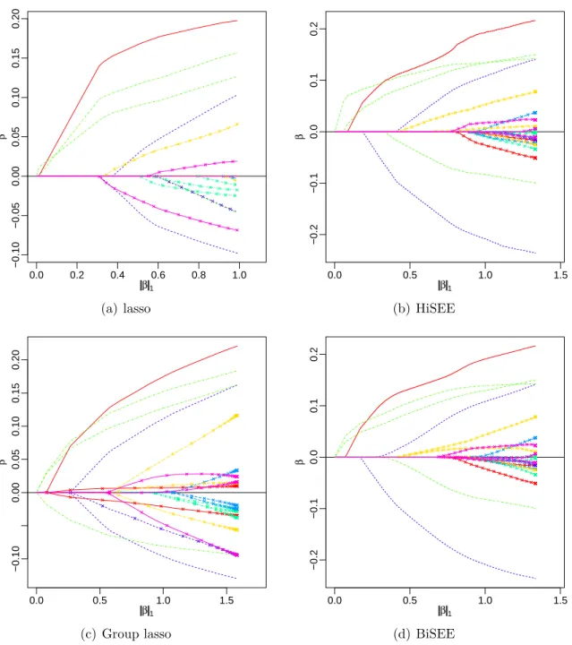
and HiSEE are able to distinguish all the important variables from the irrelevant ones. The lasso and group lasso methods are outperformed by the proposed methods mainly because they fail to utilize the bi-level variable grouping structure. First, many of the groups contain only irrelevant predictors. Considering the predictors individually, as lasso does, is wasteful and creates a greater risk of false discovery. Second, the groups that do contain useful predictors may also contain irrelevant ones. However, group lasso can only include or exclude a group as a whole.

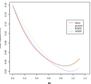
Figure 2 presents the corresponding paths of the mean squared prediction errors, based on 1000 replications. At first, all paths are comparable, but later on, the stagewise approaches, especially HiSEE, achieve lower mean predictive errors than lasso and group lasso.

2.4 Numerical Studies

We consider a longitudinal setting with cluster sizeki =k = 4 and covariates in groups of

size pj =p0 = 24. Both low and high dimension settings are considered, with (n, p, J) =

(100,72,3) and (n, p, J) = (50,216,9), respectively. Each set of p0 covariates in the same group is generated from a multivariate normal distribution with mean zero and

covariance matrix Σxof an exchangeable correlation structure, with off diagonal elements

ρx = 0.4. Three patterns of group sparsity are investigated: (I) no sparsity, (II) moderate

(47)

0.0 0.2 0.4 0.6 0.8 1.0 −0.10 −0.05 0.00 0.05 0.10 0.15 0.20 β1 β (a) lasso 0.0 0.5 1.0 1.5 −0.2 −0.1 0.0 0.1 0.2 β1 β (b) HiSEE 0.0 0.5 1.0 1.5 −0.10 0.00 0.05 0.10 0.15 0.20 β1 β (c) Group lasso 0.0 0.5 1.0 1.5 −0.2 −0.1 0.0 0.1 0.2 β1 β (d) BiSEE

Figure 1: The illustration example: paths of individual coefficient estimates against

the `1 norm of the estimates, generated by lasso (a), HiSEE (b), group lasso (c), and

BiSEE (d). All the paths are plotted against the `1 norm of the solution, e.g., kβkb ₁,

along the path. Each grouped coefficients share the same line style. Paths of irrelevant predictors are marked with “x” and those of important predictors are left unmarked.

(48)

0.0 0.2 0.4 0.6 0.8 1.0 1.2 0.02 0.04 0.06 0.08 0.10 0.12 0.14 0.16 β1

Mean Squared Error

lasso gLasso BiSEE HiSEE

Figure 2: The illustration example: the path of mean prediction error as a function of

the `1 norm of the coefficient estimates, generated by lasso, group lasso, HiSEE, and

BiSEE, averaged over 1000 replicates.

always set to bep0 = 24, with all the corresponding regression coefficients set to be 1; all other covariates have zero regression coefficients. In (I) thep0covariates in the first group

are set as the important covariates, in (II) there are p0/2 = 12 important covariates in

each of the first two groups, and in (III), there arep0/3 = 8 important covariates in each

of the first three groups. Finally, eachk×1 response vector for each cluster is generated

from the multivariate normal distribution with mean Xiβ (where the intercept value

is β0 = 1) and covariance matrix Σy of an exchangeable correlation structure, i.e., Σy

has diagonal elements σ2

y and off diagonal elements σy2ρy. The variance σy2 is chosen

to fix the signal to noise ratio (SNR) to be 2, where SNR = PJ

j=1β

>

IjΣxβIj/σ

2

y. We

consider ρy ∈ {.3, .6}, corresponding to moderate and high within-cluster correlations.

(49)

The methods to be compared with BiSEE and HiSEE include group lasso (gLasso)

and sparse group lasso (sgLasso), which have been implemented in R packageSGL(Simon

et al., 2013a). In BiSEE and HiSEE, we use exchangeable working correlation, and set

the number of iterations as N = 2000 and the step size as = 0.05. For BiSEE and

sgLasso, the tuning parameters are set to beλ2 = 1−λ1, whereλ1 ∈ {0,0.1, . . . ,0.9,1}. To compare all methods fairly, they are tuned based on independently generated testing data of large size. Specifically, the prediction error of a given solution on a given solution path/surface is defined asPñ_i₌₁( ˜Yi−µî)>Vi−1( ˜Yi−µî)/n˜, where {Y˜i, i= 1, . . . ,n˜ = 10n}

denotes the testing data, ˆµi denotes the prediction of ˜Yi based on the fitted model, and

Vi = Σy. The solution with the lowest prediction error in each solution path/surface is

then selected as the final solution for that path/surface. We also use the lowest prediction error as a predictive measure for comparing different methods. The prediction error of an oracle estimator, obtained by fitting GEEs with the true set of important covariates, is also computed. To evaluate the variable selection performance, we report both the false positive rate and the false negative rate. The false positive rate is the percent of true zero coefficients that were identified as non-zero. The false negative rate is the percent of true non-zero coefficients that were identified as zero.

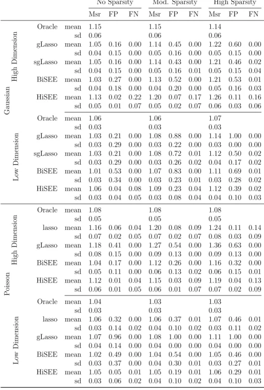
Table 1 reports the simulation results when ρy = 0.3; results when ρy = 0.6 are

provided in Table 2. Figure 3 shows the boxplots of the predictive measure. Across all simulation settings, BiSEE has the lowest predictive measure among all competing techniques. HiSEE’s predictive performance is close to, or better than, that of either

(50)

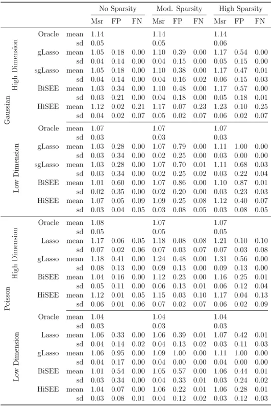
Table 1: Simulation results with ρy = 0.3 from 100 replicates. Reported are the mean

and standard deviations (sd) of the predictive measure (Msr), the false positive rate (FP), and the false negative rate (FN).

No Sparsity Mod. Sparsity High Sparsity

Msr FP FN Msr FP FN Msr FP FN Gaussian High Dimension Oracle mean 1.15 1.15 1.14 sd 0.06 0.06 0.06 gLasso mean 1.05 0.16 0.00 1.14 0.45 0.00 1.22 0.60 0.00 sd 0.04 0.15 0.00 0.05 0.16 0.00 0.05 0.15 0.00 sgLasso mean 1.05 0.16 0.00 1.14 0.43 0.00 1.21 0.46 0.02 sd 0.04 0.15 0.00 0.05 0.16 0.01 0.05 0.15 0.04 BiSEE mean 1.03 0.27 0.00 1.13 0.52 0.00 1.21 0.53 0.01 sd 0.04 0.18 0.00 0.04 0.20 0.00 0.05 0.16 0.03 HiSEE mean 1.13 0.02 0.22 1.20 0.07 0.17 1.26 0.11 0.16 sd 0.05 0.01 0.07 0.05 0.02 0.07 0.06 0.03 0.06 Lo w Dimension Oracle mean 1.06 1.06 1.07 sd 0.03 0.03 0.03 gLasso mean 1.03 0.21 0.00 1.08 0.88 0.00 1.14 1.00 0.00 sd 0.03 0.29 0.00 0.03 0.22 0.00 0.03 0.00 0.00 sgLasso mean 1.03 0.21 0.00 1.08 0.72 0.01 1.12 0.50 0.02 sd 0.03 0.29 0.00 0.03 0.26 0.02 0.04 0.17 0.02 BiSEE mean 1.01 0.53 0.00 1.07 0.83 0.00 1.11 0.69 0.01 sd 0.03 0.34 0.00 0.03 0.23 0.01 0.03 0.28 0.02 HiSEE mean 1.06 0.04 0.08 1.09 0.23 0.04 1.12 0.39 0.02 sd 0.03 0.04 0.05 0.03 0.08 0.04 0.04 0.10 0.03 P oisson High Dimension Oracle mean 1.08 1.08 1.08 sd 0.05 0.05 0.05 lasso mean 1.16 0.06 0.04 1.20 0.08 0.09 1.24 0.11 0.14 sd 0.07 0.02 0.05 0.07 0.02 0.07 0.08 0.03 0.09 gLasso mean 1.18 0.41 0.00 1.27 0.54 0.00 1.36 0.63 0.00 sd 0.08 0.15 0.00 0.09 0.13 0.00 0.09 0.13 0.00 BiSEE mean 1.04 0.17 0.00 1.12 0.26 0.00 1.16 0.32 0.00 sd 0.05 0.11 0.00 0.06 0.13 0.02 0.06 0.15 0.01 HiSEE mean 1.12 0.01 0.04 1.15 0.03 0.09 1.19 0.04 0.13 sd 0.06 0.01 0.05 0.06 0.01 0.07 0.07 0.02 0.09 Lo w Dimension Oracle mean 1.04 1.03 1.03 sd 0.03 0.03 0.03 lasso mean 1.06 0.32 0.00 1.06 0.37 0.01 1.07 0.46 0.01 sd 0.03 0.14 0.02 0.04 0.10 0.02 0.03 0.11 0.02 gLasso mean 1.07 0.96 0.00 1.08 1.00 0.00 1.11 1.00 0.00 sd 0.04 0.14 0.00 0.04 0.00 0.00 0.04 0.00 0.00 BiSEE mean 1.02 0.49 0.00 1.04 0.54 0.00 1.05 0.46 0.00 sd 0.03 0.37 0.00 0.04 0.30 0.01 0.03 0.27 0.01 HiSEE mean 1.05 0.05 0.01 1.05 0.19 0.01 1.06 0.29 0.01 sd 0.03 0.06 0.02 0.04 0.10 0.02 0.04 0.10 0.03

(51)

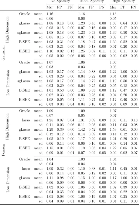
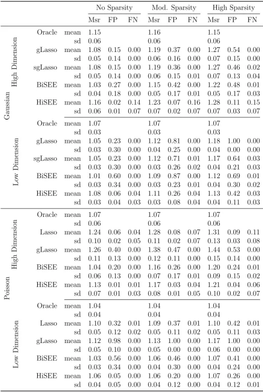
Table 2: High response correlation: simulation results with ρy = 0.6. Reported are

the average values and standard deviations of the predictive measure (Msr), the false positive rate (FP), and the false negative rate (FN).

No Sparsity Mod. Sparsity High Sparsity

Msr FP FN Msr FP FN Msr FP FN Gaussian High Dimension Oracle mean 1.16 1.16 1.15 sd 0.06 0.06 0.05 gLasso mean 1.08 0.18 0.00 1.23 0.45 0.00 1.36 0.64 0.00 sd 0.05 0.15 0.00 0.07 0.16 0.00 0.09 0.17 0.00 sgLasso mean 1.08 0.18 0.00 1.23 0.43 0.00 1.36 0.50 0.02 sd 0.05 0.15 0.00 0.07 0.16 0.02 0.09 0.17 0.04 BiSEE mean 1.03 0.31 0.00 1.18 0.47 0.00 1.30 0.52 0.01 sd 0.03 0.21 0.00 0.04 0.18 0.00 0.07 0.20 0.03 HiSEE mean 1.16 0.02 0.13 1.25 0.07 0.11 1.33 0.11 0.09 sd 0.05 0.02 0.06 0.06 0.02 0.06 0.09 0.02 0.05 Lo w Dimension Oracle mean 1.07 1.06 1.06 sd 0.03 0.03 0.03 gLasso mean 1.05 0.17 0.00 1.14 0.88 0.00 1.22 1.00 0.00 sd 0.03 0.29 0.00 0.04 0.22 0.00 0.04 0.00 0.00 sgLasso mean 1.05 0.17 0.00 1.14 0.72 0.01 1.19 0.50 0.02 sd 0.03 0.29 0.00 0.04 0.25 0.02 0.05 0.18 0.03 BiSEE mean 1.01 0.53 0.00 1.09 0.83 0.00 1.12 0.47 0.00 sd 0.02 0.33 0.00 0.03 0.28 0.01 0.04 0.20 0.01 HiSEE mean 1.08 0.05 0.04 1.11 0.27 0.01 1.12 0.40 0.00 sd 0.03 0.04 0.04 0.04 0.10 0.02 0.04 0.09 0.01 P oisson High Dimension Oracle mean 1.09 1.09 1.07 sd 0.07 0.05 0.07 lasso mean 1.25 0.07 0.04 1.31 0.09 0.09 1.35 0.11 0.13 sd 0.11 0.03 0.06 0.11 0.03 0.08 0.11 0.03 0.08 gLasso mean 1.29 0.39 0.00 1.42 0.52 0.00 1.53 0.61 0.00 sd 0.12 0.12 0.00 0.14 0.09 0.00 0.14 0.12 0.00 BiSEE mean 1.05 0.19 0.00 1.17 0.29 0.00 1.21 0.29 0.00 sd 0.06 0.14 0.00 0.06 0.16 0.01 0.08 0.14 0.01 HiSEE mean 1.15 0.01 0.02 1.19 0.03 0.04 1.22 0.05 0.07 sd 0.09 0.01 0.04 0.07 0.02 0.05 0.09 0.02 0.07 Lo w Dimension Oracle mean 1.04 1.03 1.04 sd 0.04 0.04 0.04 lasso mean 1.09 0.32 0.00 1.10 0.38 0.01 1.11 0.45 0.01 sd 0.06 0.14 0.01 0.05 0.12 0.02 0.06 0.11 0.02 gLasso mean 1.11 0.98 0.00 1.15 1.00 0.00 1.17 1.00 0.00 sd 0.06 0.09 0.00 0.06 0.00 0.00 0.06 0.00 0.00 BiSEE mean 1.02 0.56 0.00 1.06 0.50 0.00 1.07 0.39 0.00 sd 0.04 0.35 0.00 0.04 0.29 0.00 0.04 0.22 0.00 HiSEE mean 1.05 0.08 0.00 1.06 0.19 0.00 1.07 0.25 0.00 sd 0.04 0.09 0.01 0.04 0.10 0.01 0.04 0.11 0.00

(52)

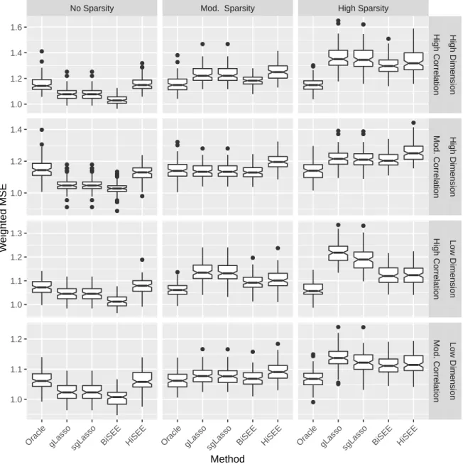
No Sparsity Mod. Sparsity High Sparsity ● ● ● ● ● ● ● ● ● ● ● ● ● ● ● ● ● ● ● ● ● ● ● ● ● ● ● ● ● ● ● ● ● ● ● ● ● ● ● ● ● ● ● ● ● ● ● ● ● ● _● ● ● ● ● ● ● ● ● ● ● ●_● ● ● ● ● ● ● ● ● ● ● 1.0 1.2 1.4 1.6 1.0 1.2 1.4 1.0 1.1 1.2 1.3 1.0 1.1 1.2 High Correlation Mod. Correlation High Correlation Mod. Correlation High Dimension High Dimension Lo w Dimension Lo w Dimension

Oracle _{gLasso sgLasso BiSEE HiSEE} Oracle _{gLasso sgLasso BiSEE HiSEE} Oracle _{gLasso sgLasso BiSEE HiSEE} Method

W

eighted MSE

(53)

group lasso or sparse group lasso. Also, the advantage of BiSEE and HiSEE becomes more visible when the response correlation increases. This is largely due to the fact that both BiSEE and HiSEE are based on GEEs, which accounts for within cluster dependence. In the no sparsity setting, we notice that the lowest predictive measure is not necessarily produced by the oracle estimator. Further investigation shows that this is because the stagewise estimators and the penalized estimators are all capable of inducing shrinkage estimation, which can be beneficial to deal with multi-collinearity. For variable selection, BiSEE yields comparable false positive rate compared to gLasso and sgLasso, and all of them have very low false negative rate. This is expected as it is known that convex penalization methods tend to select more variables when tuned based on predictive performance. HiSEE has the lowest false positive rate across all settings, at the expense of a higher false negative rate.

The study with Poisson response is similar to that with Gaussian response. The dif-ferences are described as follows. The within-cluster dependence of Poisson responses is set to be a normal copula with an exchangeable correlation structure whose off-diagonal

values are ρy ∈ {.3, .6}. The marginal Poisson distributions are set to have mean

g−1₍_X

ijβ) for thejth observation in theith cluster, whereg is the log link function. The

group size of the covariates is set to be p0 = 12, and the model dimensions in low and

high dimension settings are set as (n, p, J) = (100,36,3) and (n, p, J) = (50,216,18), respectively. The three group sparsity patterns are set in the same fashion as in the

(54)

Gaussian study, with the coefficients of p0 = 12 important variables set to be 0.1 dis-tributed in the first three groups. Since sgLasso implementation for Poisson regression is not available, we only consider lasso and gLasso in the comparison, using

implementa-tions from R package grpreg (Breheny and Huang, 2009). HiSEE and BiSEE use step

size of = 0.025. Each configuration is replicated 100 times. The performance of

differ-ent methods is still compared in terms of prediction error, false positive rate, and false negative rate, as defined earlier. In the prediction error, however,Vi, the variance matrix

of ˜Yi, is approximated asA

1/2

i R( ˆα)A

1/2

i , where ˆαis estimated from an independent data

set of size 10n.

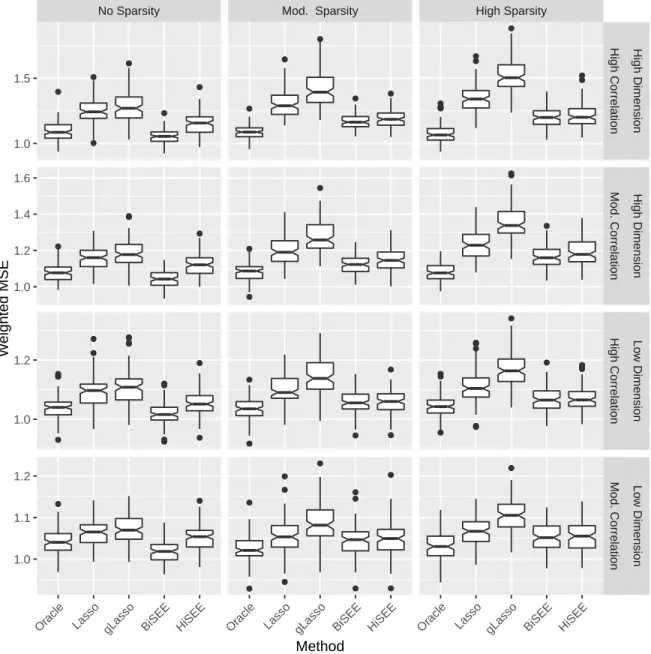
The simulation results are summarized in Tables 1 and 2. Figure 4 presents the box-plots of the predictive measures of different methods. Most observations in the Gaussian case remain. BiSEE and HiSEE outperform both lasso and gLasso in prediction. The variable selection performance of BiSEE is in between those of lasso and gLasso. HiSEE in general yields the smallest false positive rates among all methods, with well-controlled false negative rates. The advantages of BiSEE and HiSEE become more visible as the within-cluster dependence increases.

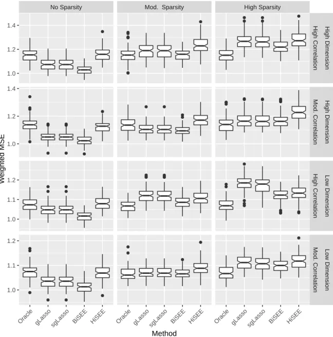
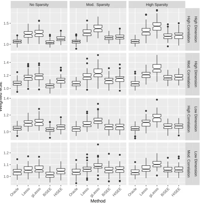
2.4.1 Between Group Correlation

We conducted an additional simulation study to examine the effect of between group correlation. All of the same simulation settings described in Section 2.4 are used with correlation induced between groups in a manner similar to that which is described in

(55)

No Sparsity Mod. Sparsity High Sparsity ● ● ● ● ● ● ● ● ● ● ● ● ● ● ● ● ● ● ● ● ● ● ● ● ● ● ● ● ● ● ● ● ● ● ● ● ● ● ● ● ● ● ● ● ● ● ● ● ● ● ● ● ● ● ● ● ● ● ● ● ● ● ● ● ● ● ● ● ● ● ● ● ● ● ● ● ● ● 1.0 1.5 1.0 1.2 1.4 1.6 1.0 1.2 1.0 1.1 1.2 High Correlation Mod. Correlation High Correlation Mod. Correlation High Dimension High Dimension Lo w Dimension Lo w Dimension

Oracle Lasso gLasso BiSEE HiSEE Oracle Lasso gLasso BiSEE HiSEE Oracle Lasso gLasso BiSEE HiSEE Method

W

eighted MSE

Stagewise Estimating Equations

Stagewise Estimating Equations

Greg Vaughan

ABSTRACT

APPROVAL PAGE

Stagewise Estimating Equations

Dedication

Acknowledgements

Contents

List of Tables

List of Figures

Chapter 1

Introduction

1.1

Overview

1.2

Literature Review

1.2.1

Penalized Regression

1.2.2

Generalized Estimating Equations

1.2.3

Stagewise Estimation

1.2.4

Model Selection with Grouped Covariates

1.2.5

Interaction Selection

1.3

Outline

Chapter 2

Stagewise Generalized Estimating

Equations with Grouped Variables

2.1

Grouped Covariates

2.2

Notation

2.3

Stagewise Generalized Estimating Equations

2.3.1

Bi-level Stagewise Estimating Equation

2.3.2

Proof of Theorem 2.1

2.3.3

Lasso and Group Lasso As Special Cases

2.3.4

Hierarchical Stagewise Estimating Equation

2.3.5

Algorithm Details

2.3.6

An Illustration

2.4

Numerical Studies

2.4.1

Between Group Correlation