Irish Mortgage Default Optionality

Irish Mortgage Default Optionality

Gregory Connor and Thomas Flavin

Department of Economics, Finance & Accounting

National University of Ireland, Maynooth

October 22, 2013

Abstract

The owner of a residential property subject to a nonrecourse mort-gage essentially has a put option against the market value of the prop-erty. If the market price of the property falls su¢ ciently, the owner can surrender the property to the mortgage issuer and in exchange receive full o¤set of the cash ‡ow liability of the mortgage loan. A similar but diluted put optionality holds for recourse mortgages if there are legal or practical limits to the mortgage issuer’s recourse claim against the owner’s future income. Previous research based on American data …nds that put optionality is an important, but not exclusive, determi-nant of mortgage default. This paper utilizes a database of troubled Irish mortgages to analyze the in‡uence of put optionality on Irish property owners’default behaviour. We …nd that put optionality is a very important explanatory variable for observed Irish mortgage de-faults, complementing and strengthening existing empirical …ndings from US mortgage markets.

We wish to acknowledge support from the Science Foundation of Ireland under grant 08/SRC/FM1389. We would like to thank Permanent TSB for provision of the data used in this study; Liam Delaney, Conall MacCoille, Donal O’Neill, and participants at the National University of Ireland Maynooth economics seminar and the Dublin Economics Workshop for helpful comments; and Anita Suurlaht for excellent research assistance.

y_{Connor: Tel. (353) 1 708-6662, Email. [email protected]; Flavin: Tel. (353) 1}

1

Introduction

The owner of a residential property subject to a nonrecourse mortgage who is willing to renege on his loan essentially holds a put option against the market value of the property. If the market price of the property falls su¢ -ciently, the owner can surrender the property to the mortgage lender and in exchange receive full o¤set of his cash ‡ow liability from the mortgage loan. In options terminology, the homeowner has a long-term American put option on a dividend-paying asset (the implicit rental yield of the property serves as the dividend ‡ow) with exercise price equal to the cash-equivalent value of the mortgage liability. The moneyness of the put option is one minus the reciprocal of the loan-to-value ratio of the mortgage. A similar, but diluted, put optionality holds for recourse mortgages, since there are legal and prac-tical limits to a mortgage lender’s recourse claim against the owner’s future income, for example, relief from this claim through personal bankruptcy. In most situations, both the homeowner and mortgage lender incur substantial transactions costs upon exercise by the homeowner of this put option. This two-sided transactions-cost feature of the put option leads to a bargaining game between the homeowner and mortgage lender, with the homeowner po-tentially able in some circumstances to gain mortgage payment concessions by threatening to surrender the asset but not doing so. The bargaining power of the mortgage borrower in default seeking repayment concessions increases with the moneyness of the put option.

Particularly in the case of a recourse mortgage, there are reputational costs and social/ethical considerations for the homeowner from defaulting, since in doing so the homeowner has violated the terms of an agreed contract for personal gain. In many cases, the mortgage lender will continue to re-ceive (more valuable) required mortgage payments even when options theory predicts that it will be forced to accept surrender of the property.

Most existing Irish residential mortgages are contractually written to be full recourse and with unhindered security against the property. However, in recent years a number of legislative and regulatory changes have altered the

de facto nature of mortgage claims. Irish residential mortgages are now, in practice, limited-recourse contracts and have strictly limited security against the property asset, and high transactions costs for the mortgage lender in exercising the security claim. Given the extremely large falls in Irish res-idential property values during the period 2008 to 2012, it is sensible to examine whether put optionality helps to explain the explosive increase in

Irish mortgage arrears over roughly that same period.

This paper empirically examines the in‡uence of put optionality on the default behaviour of Irish mortgage borrowers. We rely on a large database of Irish mortgages provided to us by a mortgage lender in Ireland, Permanent TSB. The database covers all mortgages at Permanent TSB for which the holder has submitted a Standard Financial Statement (SFS), giving a sample of 28,377 mortgage accounts. Submitting an SFS is a required component of the Central Bank of Ireland’s mandated mortgage arrears resolution process (MARP). The entry of a mortgage borrower into MARP is either at the initiation of the bank after one or more missed mortgage payments or, less commonly, by the mortgage borrower looking to engage with the bank for help with their mortgage payment di¢ culties. The sample is doubly-censored since it consists only of mortgages which have been brought into MARP, and does not include troubled mortgages which should be in MARP but where the mortgage borrower has refused to submit the required SFS. Our data panel consists of information from the SFS collated with information from the original loan application and some other loan-speci…c data items. Roughly half the mortgages in our sample are in default, de…ned as greater than 90 days worth of accumulated payment arrears, and half are not in default.

Our main empirical task is to build a model explaining which of this ob-served subset of all mortages, that is the subset of mortgages in MARP where the mortgage borrower has submitted an SFS, are in default, and which are not in default. We use a combination of analysis of variance, multivariable probit models and nonparametric and semiparametric kernel-based estima-tors. We …nd that put optionality is a signi…cant explanatory variable for Irish mortgage default. The loan-to-value ratio, which measures the money-ness of the implicit put option, is the most powerful variable in generating di¤erences in average default rates across portfolios of loans double-sorted by levels of explanatory variables. In a multivariate probit model of mort-gage default, loan-to-value is again the most important explanatory variable, measured by marginal contribution to the probability of default. The put-optionality e¤ect is particulary strong when combined with household income stress, supporting the "dual trigger" model of mortgage default. Whereas in US data, a¤ordability is generally found to be more important than put-optionality as a predictor of default, within our (doubly-censored) Irish sam-ple, put-optionality appears more important than a¤ordability as a predictor of default.

for an options-type convexity in the functional link of loan-to-value to mort-gage default probability. This convex relationship also conforms to …ndings in US-based research on the e¤ect of loan-to-value on mortgage default rates. Section two reviews the existing literature and critically examines the insights which options theory can provide regarding mortgage default behav-iour in Ireland. Section three describes our econometric model of mortgage default. Section four empirically examines the default behaviour of mort-gages in our database. Section …ve summarizes the paper.

2

Optionality and Mortgage Contracts

There is a large research literature examining the impact of the implicit put option in mortgage contracts on default behaviour by mortgage borrowers. The empirical component of this research is mostly based on US mortgage market data. We will brie‡y review a few of the papers with particular relevance.

The original insight for modeling mortgage default as a put option is cred-ited to Asay (1978). Deng et al. (2000) show empirically that a continuous-time, frictionless market, Black-Scholes-type theory of mortgage default as put option exercise provides useful empirical content, but is not su¢ cient as an empirical model. Unlike the exercise of a securities-market traded put option on a stock, defaulting on a mortgage has large …xed costs, and a po-tentially large impact on the future economic opportunities of the mortgage borrower, particularly through its impact on their personal credit rating and the availability of new mortgage …nance to them. Deng et al. also note that mortgage default is not fully "rational" in the sense of cash-‡ow maximizing – there are moral/social/psychological aspects to the default decision. Most of the recent literature does not rely on the continuous-time, frictionless market assumptions of Black-Scholes type models.

Elmer and Seelig (1998) build a model of mortgage default which com-bines both inability-to-pay and put-optionality as causes of default. Us-ing US data aggregated at the state and regional level, they …nd that both causes play a role in mortgage default, but that inability-to-pay is relatively stronger. The data used in the paper pre-dates the volatile US property price declines of the post-2007 period.

Using loan-level data, Tirupattur et al. (2010) conclude that defaults driven by negative equity, rather than ability to pay, are a signi…cant

phe-nomenon in US residential mortgages over their sample period. A borrower is de…ned as strategically in default (that is, exercising their put option) when their mortgage goes from current to 30-, 60- and then 90-days in arrears without any payment during this period or any subsequent payments, while the borrower continues to service non-mortgage loans. Strategic defaults in-crease over time in concert with the decline in US residential property prices and by the end of the sample (February 2010), they represent 12% of all defaulted mortgages. Wyman (2009) uses a similar approach and estimates that by second quarter of 2009, 19% of all defaults were strategic.

Bhutta et al. (2010) build a theoretical model of mortgage borrower default decisions combining inability-to-pay and put-optionality reasons for default. They test the model using a loan-level database, combined with micro-regional property price indices, covering several US states with large property price declines (and business cycle recessions) in the post-2007 pe-riod. They …nd that, considered separately, inability to pay is the more important source of default decisions, but that put optionality also plays a prominent role. They …nd that when negative equity exceeds 50 percent of the property’s value, half of the defaulters are exercising their put option rather than experiencing any inability to pay. Also, Bhutta et al. argue that their empirical …ndings support Foote’s (2008) "dual-trigger" model of default –default is highest when householders experience both simultaneous income fallsand negative equity increases. The two causes of default interact and reinforce each other.

Bhutta et al. note that a contributory factor in strategic default is the long "free-rent" period between original default and repossession; this period lasts at least eight to twelve months in most US states, dependent upon the speci…c legal statutes of the state. The implicit cash value of the free-rent pe-riod adds to the put-optionality payo¤ from default and further incentivizes strategic default. Cutts and Merrill (2008) look in detail at cross-state dif-ferences in the length of the free-rent period associated with necessary legal delays in the repossession process. They …nd that states with relatively shorter periods have generally better outcomes in terms of cure-rates (the proportion of households with mortgages in arrears that get back on track and keep their property). They estimate an "optimal" repossession interval of 270 days from original missed payment to physical repossession, consist-ing of 150 days of customer counselconsist-ing/assistance with mortgage arrears, a default declaration notice by the lender, and then 120 days before physical repossession.

Relying on survey data, Guiso et al. (2011) …nd that social considerations, such as morality and fairness, in‡uence borrowers on the acceptability of strategically defaulting. They estimate that in their sample 26% of existing defaults are strategic. They …nd that almost no households will deliberately choose to default (given ability to pay) if negative equity shortfall is less than 10% of the value of the house; 17% of households will choose to default even if they can a¤ord to pay their mortgage when negative equity reaches 50% of the value of the property. Burke and Mihaly (2012), also based on survey data, …nd that social perceptions about the acceptability of strategic default, and …nancial literacy (the ability to navigate the US bankruptcy system) in‡uence household’s tendency toward strategic default. Seiler et al. (2012) report that networks are an important determinant of strategic default: borrowers who have family and friends in default are more likely to strategically default themselves. Towe and Lawley (2010) also …nd that social interactions play a signi…cant role in the decision to default, in that having a neighbour in foreclosure increases the probability of default by 28%. Elul et al. (2010) use an econometric framework somewhat similar to our own. They de…ne default as accumulated arrears of 60 days or more, and estimate a logit model of binary default outcomes based on individual-credit-record data, together with nationwide quarterly interest rate data and quarterly US state-level unemployment rate changes. They …nd that both negative equity, which they interpret as put-optionality, and inability to pay have a signi…cant e¤ect on mortgage default probability. They also …nd that the two causes interact, so that mortgage default rates are particularly high when negative equity is combined with stressed ability to pay. Elul et al. also explore the possibility of a nonlinear impact of negative equity on mortgage default rates and …nd some con…rmatory evidence.

Trautmann and Vlahu (2011) build a game-theoretic model of borrower runs: the tendency of borrowers to deliberately choose default when they perceive balance sheet weakness at the lending bank. Borrowers know that weak banks are likely to be less aggressive in quickly repossessing property, and also that the long-term relationship of the borrower with the bank has less value if the bank is weak. Since borrower loan nonpayments aggravate the weakness of the bank’s balance sheet, borrower runs can self-reinforce in the same way as bank depositor runs.

The bargaining-game perspective of Trautmann and Vlahu highlights an important bargaining-game bene…t to strategic default which increases as the moneyness of the implicit put option increases. Mortgage borrowers are

aware that the lending bank must pay a large transactions cost in repossessing a property, and that the bank would bene…t if it could negotiate reduced-value payment terms rather than repossess a negative-equity property. If the bank does not have full recourse to all the borrower’s future income, then negative equity in the loan creates a gap between the present value of full mortgage payments and the present value of the minimum mortgage pay-ments that the bank will hypothetically accept to avoid costly repossession. Strategic default (particularly in Ireland where repossession is very costly and di¢ cult for banks) can be employed as a credible threat in negotiations for improved payment terms. Given the structure of Irish mortgage contracts (limited recourse, very costly repossession, banks with weak balance sheets) this is likely to be an important consideration in the Irish case.

Lydon and McCarthy (2011) provide an analysis of Irish mortgage market default based on data collected from four Irish banks during the Central Bank of Ireland’s 2010 stress-testing review of the domestic banking sector. Like Elul et al. (2010) and this paper they use a static probit model of mortgage default based on individual loan characteristics. They argue that their static probit model results support a ‘dual-trigger’ model of default in which both a¤ordability and put-optionality (that is, high loan-to-value ratios) impact household mortgage default. They also …nd that the regional unemployment rate, as a proxy for local economic shocks, has an impact on regional average default rates. Using a dynamic model applied to regional loan portfolios rather than individual loans, they can not con…dently identify a put-optionality e¤ect on default for regional home loan portfolios, but the e¤ect is statistically signi…cant for regional buy-to-let loan portfolios.

One obvious concern is the applicability of US-based research for mod-eling the default behaviour of Irish mortgage borrowers. There are impor-tant social, cultural, regulatory, and legal di¤erences between U.S. and Irish residental mortgage markets. The Irish legal and regulatory environment has not been constant over the our sample period. Starting with the 2009 Land Reform Act, which contained a legal ‡aw rendering residential prop-erty repossession virtually impossible in Ireland, there have been a variety of changes to repossession, bankruptcy, and personal insolvency laws and regulation. The legal ‡aw in the 2009 Land Reform Act was eventually re-moved after sustained pressure from Ireland’s international lenders under the sovereign bail-out programme (the International Monetary Fund, European Central Bank and European Union). From an international perspective, the current Irish system is borrower-friendly and repossession is slow and costly;

see Mac Coille et al. (2013) for a review. Coincidentally or otherwise, dur-ing the economically-turbulent period in which these regulatory and legal changes to mortgage contract enforcement were implemented, Irish mort-gage arrears grew explosively. Figure 1 compares the time-series patterns of Irish mortgage defaults, the unemployment rate, per capital real income, and residential property prices over the period Q4 2002 - Q2 2013; all the series are normalized to 100 at the starting date of mortgage default data availability, Q3 2009.

3

Linear, Nonparametric, and Partially

Lin-ear Index Probit Models of Mortgage

De-fault in a Panel Dataset

3.1

Linear Index Probit: A Brief Review

Our basic econometric model is a linear-index probit model of default. We assume that for each mortgage, the mortgage borrower’s default outcome is based on an unobserved (by the econometrician) decision index vi; ifvi >0

then the mortage holder defaults. Each mortgage borrower’s decision index is a linear combination of a k vector of explanatory variables xi with linear

coe¢ cients plus an unobservable individual-speci…c random component "i

capturing default-relevant idiosyncratic e¤ects:

vi = 0+ 0xi+"i (1)

and we assume that"i has a standard normal distribution and is independent

across mortgage borrowers. Let di denote the observable binary variable

which is 1 if the mortgage borrower has defaulted and0otherwise. Let ( )

denote the cumulative probability function of a standard normal variate. Given observation of_fdi; xigi=1;:::;n maximum likelihood estimation of( 0; ) is straightforward: ( 0; ) = arg max ( 0; ) 1 n n X i=1 dilog( ( 0+ 0xi))+ (2) (1 di) log(1 ( 0 + 0xi))

which is easily solved by nonlinear maximization and gives consistent, as-ymptotically normal estimates with consistently-estimated standard errors,

see, e.g., Greene (2000). The empirical results will be presented in the next section. Readers who are not interested in the econometric technicalities re-quired to allow nonlinearity in the decision index (1) may wish to skip ahead to that section.

3.2

Nonparametric Estimation of the Link between

Loan-to-Value and Default

A potential weakness of standard probit, in our application, is the assumption of a linear decision index (1). Options pricing theory predicts that the put-option component of the value of default depends nonlinearly upon the loan-to-value ratio. The exact nonlinear shape is not possible to derive due to the complexity of the embedded put option. The put-option-based value of default is near zero for loan-to-value below one and then slopes positively. There is corresponding empirical evidence from US research that strategic mortgage default is nonlinear in the loan-to-value ratio, which again argues against the linearity assumption in the decision index.

In this subsection we analyze a probit model with a fully nonparametic decision index. This model is theoretically estimable by maximum likelihood, see Matzkin (1992), but it is not feasible in our application due to the curse of dimensionality (we have six explanatory variables). Nonetheless we can use the general model to estimate the conditional expected rate of default as a function of loan-to-value. This conditional expectation function is estimable, and can be compared to the predicted conditional expectation function im-plied by the linear-index probit model. Comparison of the two estimates of this conditional expectation function provides the basis for a nonparametric test of index-linearity of the probit model. We are able to test the linear-index probit model against a general nonparametric alternative without being able to completely estimate the nonparametric alternative.

We replace the linear decision index with a nonlinear generalization:

vi =f(xi) +"i (3)

where f( ) is a thrice continuously di¤erentiable multivariate function. We continue to assume that"ihas a standard normal distribution and is

indepen-dent across i. We assume that for eachi the vector of explanatory variables

xi is a realization from a multivariate joint distribution, independent of "i :

with the restrictions on D described later. Let the …rst component of xi;

that is x1i; be the loan-to-value ratio. Note that conditional upon a realized

value of xi and given knowledge of f( ); the probability distribution for di

has the same form as in the case of linear-index probit:

Pr(di = 1) = (f(xi));

recall that ( )denotes the cumulative normal probability function. Sincedi

is a binomial zero-one this implies:

E[dijxi] = (f(xi)):

Recall that we assume thatf( )is a smooth multivariate function. We require that the joint density of the explanatory variables, D, is su¢ ciently smooth so that the following conditional expectation is well-de…ned and thrice con-tinuously di¤erentiable in xi1:

g(x1i) =E[E[dijxi]jx1i] =E[ (f(xi))jx1i]: (4)

Nonparametric regression provides a natural method for estimating g(x1i)

based on the conditional moment expression (4). In large samples, the con-ditional expected default at a particular point x1i is consistently estimated

by the local-weighted average default in the neighbourhood of x1i :

plim n!1 1 Sn n X j=1 dj (x1j; x1i) = g(x1i) (5) where (x1j; x1i) =dens( x1j x1i

hn )for some density functiondens( )and

band-width hn, and sum of weights Sn = n

P

j=1

dj (x1j; x1i): See the Technical

Ap-pendix for conditions guaranteeing the consistency and asympotic normality of the estimator (5).

Note that this fully nonparametric model encompasses the linear-index probit model as a special case. This allows us to test the linear decision index against a fully nonlinear alternative without maximum likelihood estimation of (3). First estimating the linear index probit model by maximum likeli-hood (2), we then use the same kernel regression to estimate the conditional expectation function using the estimated linear index probit model. Any di¤erence between these two nonparametric estimates of the conditional ex-pectations function captures a linear model bias of the probit model. Under

the joint assumptions of this subsection and of the probit model in subsection 3.1 above: plim n!1 1 Sn X (b0 +b0xj) (x1j; x1i) =g(x1i) (6)

where the kernel regression terms are identical to (5) above. See the Technical Appendix for conditions guaranteeing consistency of the estimator (6). The di¤erence between the unrestricted (5) and restricted (6) estimates of g(x1i)

we call the linear model bias.

3.3

Partially Linear Index Probit: A Brief Review

There are a number of semiparametric extensions of the standard linear pro-bit model, designed to add ‡exibility to the functional form without unduly sacri…cing estimation accuracy. The partially linear index probit model is a particulary appropriate model choice in our application. It sacri…ces some of the ‡exibility of the fully nonparametric model discussed in the last sub-section, by imposing linearity for all but one of the explanatory variables. The decision index is assumed to take the following additive semiparametric form:

vi =f(x1i) + (1)0 x(1)i +"i (7)

where x(1)i is a (k 1) vector of the explanatory variables excluding the

loan-to-value ratio x1i and (1)is a(k 1) vector of associated linear coe¢ -cients. The univariate function f(x1i) is assumed to be thrice continuously

di¤erentiable, and "i is standard normal. The intercept 0 is not included in the model since it is not identi…ably separable fromf(x1i).

We follow the estimation algorithm proposed by Carroll, et al. (1997). To get initial values, the linear-index probit model (1) is estimated by maximum likelihood (2). Then for a grid point x1i a local quasi-maximum likelihood

problem is solved for scalar estimate fbx1i :

b fx1i = arg max 1 Sn n X i=1 (x1i; x1i)fdilog( (fbx1i +b 0 (1)x(1)i))+ (8) (1 di) log(1 (fbx1i +b 0 (1)x(1)i))g

where (x1i; x1i)is a kernel-weighting scheme andSnis the sum of the kernel

a set of …nely spaced grid points covering the sample range of x1i: A

cross-section of implied estimates forf(x1i)is found by interpolating between grid

points:

b

f(x1i) =fbx1i+ (x1i x1i)(fbx1i fbx1i) (9)

where x_1i > x1i are the two contiguous grid points containing x1i: Next, we

return to the linear-index probit maximum likelihood problem but replacing 0+ 1x1i with the pre-estimated f(xb 1i)from (9):

b₍₁₎ = arg max (1) 1 n n X i=1 dilog( (f(xb 1i) + (1)0 x(1)i))+ (10) (1 di) log(1 (fb(x1i) + (1)0 x(1)i)):

The two steps (8) and (10) are iterated to convergence. See Carroll, et al. (1997) and Bellemare, et al. (2002) for discussion of convergence properties, optimal bandwidth choice, and related issues. Our estimates appear in the next section.

4

Empirical Analysis of Irish Mortgage

De-faults

4.1

The Database and Key Variables

Our database was provided by Permanent TSB bank and consists of all prop-erty loans at Permanent TSB that have submitted a Standard Financial Statements (SFS). The bank collates the information in the SFS with exist-ing bank information on the loan account, includexist-ing application information and payment records.

The Central Bank of Ireland mandates that all mortgage lenders must col-lect an SFS from each home loan mortgage borrower in arrears, as part of the Mortgage Arrears Resolution Process (MARP). MARP is the Central Bank mandated process that all regulated mortgage lenders must follow in deal-ing with customer mortgage payment di¢ culties. Each regulated mortgage lender must treat every loan which has been arrears of any amount for more than 31 calendar days as in MARP and must write to the mortgage borrower within 3 business days after these 31 days are elapsed and tell them that they are covered by MARP. The lender must provide an SFS to the borrower in

MARP, give them assistance in …lling out the SFS as needed, and then must pass the completed SFS to the Arrears Support Unit within the lending bank which must follow speci…c regulations in dealing with each MARP case. If the mortgage borrower fails to return the SFS then they can be classi…ed under Central Bank of Ireland regulations as a noncooperative borrower and borrower protections under MARP may be lifted. Mortgage borrowers may also voluntarily submit an SFS, for example in order to negotiate mortgage restructuring without falling into arrears.

There are a total of 28,377 loan accounts in the database, 25,235 home loan accounts and 3,142 residential property investor loan accounts (called buy-to-let loans). Mortgage borrowers with both home and buy-to-let loans are included in the buy-to-let loans …gure. For each multiple-loan account we aggregate the individual loan characteristics and e¤ectively treat it as one loan observation. Taking account of borrowers with multiple loans the database covers 37,547 individual home loans and 4,285 individual buy-to-let loans; this compares to a total outstanding portfolio of 140,060 home loans and 23,133 buy-to-let loans at Permanent TSB, so 23.7% of the bank’s total home loans portfolio are in the database and 18.5% of its buy-to-let loans portfolio. The database includes a default dummy for any loan that has accumulated arrears of greater than 90 days. A multiple account is treated as in default if accumulated arrears on any of the loans is greater than 90 days of required payments. Table 1 shows the percentages of the two loan types in default in the database. In the Permanent TSB total loan book, 15.3% of home loans and 17.9% of buy-to-let loans are in default; this of course di¤ers sharply from our database (SFS-linked loans only) with 48.7% for home loans and 49.9% for buy-to-let loans in default.

In addition to the default dummy, the database has the "number of days" of accumulated arrears (30 x arrears amount/monthly required payment). Table 2 summarizes this data. This measure has the advantage over the de-fault dummy that it captures the level of accumulated arrears rather than only giving a binary indicator of default. However, the range of values runs very high - half of the mortgages in arrears have almost a year (314 days) of accumulated arrears. The di¤erence between a loan that is …ve years in arrears and a loan which is one year in arrears seems mostly a matter of timing for when the default began, rather than a di¤erent decision by the mortgage borrower. Also, there is extant research literature on mortgage loan default but no comparable non-Irish data or research on multi-year ac-cumulated arrears. Hence we focus on models explaining loan default rather

than accumulated arrears.

There are two sources of censoring in our database, both of which limit the general applicability of our empirical analysis. First, we only have informa-tion on mortgages for which there is an SFS on …le at the bank. Completely non-distressed mortgages do not appear in our database, and so we do not model their holders’decision-making in choosing non-default.

The second source of censoring comes from imperfect compliance with the Central Bank of Ireland requirement for an SFS for each troubled mort-gage. It is not possible from the database to compute the compliance rate for all mortgage types since SFS submissions can be required by the bank or voluntarily chosen by the mortgage borrower. One exception is home mort-gages in default, where submission of an SFS is mandated in all cases by MARP. Permanent TSB records 21,398 home loan accounts in default, but they have only 14,996 SFS submissions from home loan mortgage borrowers in default, giving a SFS submission compliance rate of 70.1% for this sub-category. The potential statistical interaction between the non-cooperation decision of mortgage borrowers in arrears and our model of their mortgage default decision (based only on data for those who have complied) limits the applicability of our results for mortgages outside the conditioning set. It seems possible that non-cooperation is more tempting for borrowers with cer-tain characteristics, and these characteristics may also impact their default decision-making. We can only o¤er the caveat that our model is of borrower default outcomes conditional upon their submitting an SFS, and is not de-pendable for non-cooperating borrowers, who are outside this conditioning set.

We rely on six explanatory variables for loan default. Application LTV is the loan-to-value ratio at the time the loan was issued (we also have the date of issue, which we use in Table 3 below). LTV is the estimated current loan to value ratio. The current loan to value ratio takes the most recent physical valuation of the property available to the bank (for the majority of loans this will be the valuation done at the application date, but it may be more recent) and then uses a property price index to adjust forward the valuation to account for price increases and/or decreases since the physical valuation date. The forward price adjustment uses the most relevant of the following four property price indices for each individual property: Dublin houses, Dublin apartments, non-Dublin houses, and non-Dublin apartments. The loan amount is adjusted for amortization or reverse-amortization of the capital balance using the bank’s payment records on the individual loan.

The payment to income index, or a¤ordability index for short, is de…ned as required payment commitments divided by net income. Net income is the after-tax income of the borrower (or multiple borrowers). The de…nition of required payment commitments di¤ers between home loans and buy-to-let loans:

Required payment commitments for home loans = existing short term debt payments + existing mortgage payments + existing buy-to-let de…cit + maintenance costs + proposed buy-to-let de…cit + proposed mortgage payments - tax relief.

Required payment commitments for buy-to-let loans = existing short term debt payments + existing mortgage payments + existing buy-to-let de…cit + maintenance + proposed buy-to-let de…cit - tax relief.

The same formulas are used for the application values and current values of the a¤ordability index. The current values are at the date on which the most recent Standard Financial Statement was received, and use information provided by the household on the SFS.

The loan-to-value ratios for a multiple-loan account are computed as the sum of the multiple loan amounts divided by the sum of the property values, both currently and at the application date of the most recent loan. The a¤ordability ratio for a multiple-loan account sums the required payment commitments from all the loans and then divides by net income.

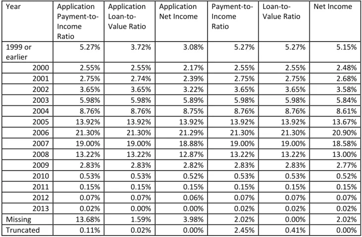
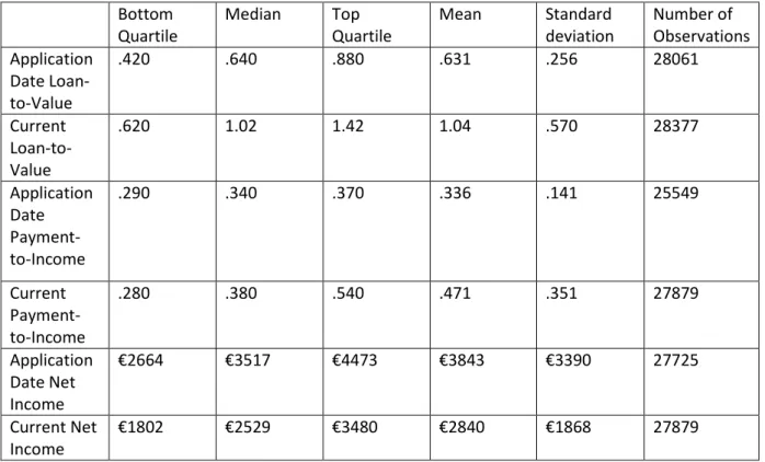
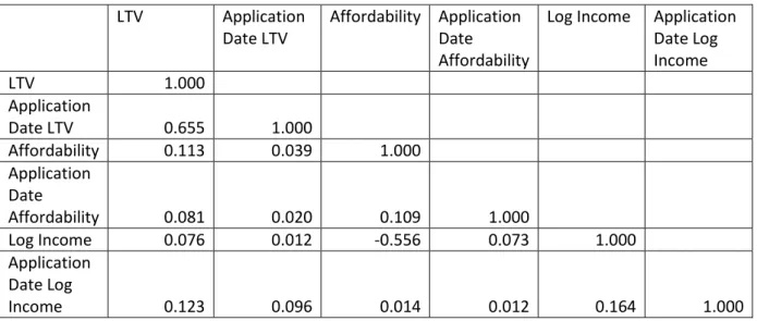
We examined the database for data outliers and other discernible errors. The only notable problem we could identify was that 0 had been used in some cases in place of missing data. Since all six of our explanatory variables should be strictly positive, except in most unusual circumstances, we treat all zero entries as missing. We truncated application LTV and LTV at 5.0, and the a¤ordability index at 3.0, to dampen the in‡uence of extreme values (which may be data errors) on the estimation routines. Table 3 shows the number of mortgage entries in our database for each year of loan origination, along with the number of data points truncated. The columns in the table di¤er since some variables have missing data, particularly for application data at earlier loan origination dates. Sixty-seven percent of the mortgages in the database originate in the four years 2005-2008. Table 4 provides descriptive statistics on the six explanatory variables. Table 5 shows the correlation matrix of the explanatory variables.

4.2

Estimation of the Model

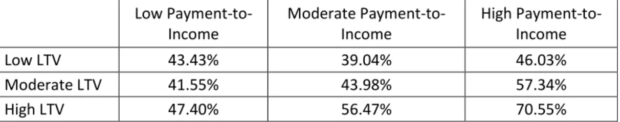
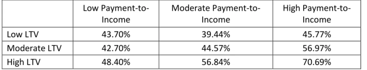
As a preliminary step we double-sort all loans using each pair of the three current variables: loan-to-value, payment-to-income, and log income, and then compute the average default rate within each subset. For each variable the …rst breakpoint is the 25% fractile of its univariate distribution and the second breakpoint is the 75% fractile, so that the middle category captures the interquartile range. The interquartile range is (0:62;1:42) for loan-to-value, (0:28;0:54) for payment-to-income, and (log(1;802);log(3;480)) for log of net monthly income. The results appear in Table 6. All three of the variables seem to contain information about default rates. The strongest double-sort comes from using loan-to-value and log income together, but all three variables show some explanatory power. The corresponding tables for home loans and buy-to-let loans examined separately are shown in the supplementary tables in the appendix.

The results in Table 6a are particularly interesting. For purposes of infor-mal analysis the three columns in the table can be thought of as a¤ordable payment, stressed payment, and una¤ordable payment; the three rows can be thought of as positive equity, zero to moderate negative equity, and large negative equity. Note that the (1;1) subset (a¤ordable payment, positive equity) has an average default rate of 43.4% whereas the (3;3) subset (un-a¤ordable payment, large negative equity) has a default rate of 70.6%. The

(3;1) and (1;3) subsets have roughly equal average default rates which are not that much higher than for the(1;1)subset. The big jump in the default rate comes when the loan has both low a¤ordability and large negative eq-uity: the joint e¤ect seems much bigger than the sum of the two individual e¤ects. This conforms to Foote’s (2008) dual-trigger model of default, and supports the US-based …ndings of Bhutta et al. (2010) and Elul et al. (2010). The probit model which we use below also captures this empirical feature.

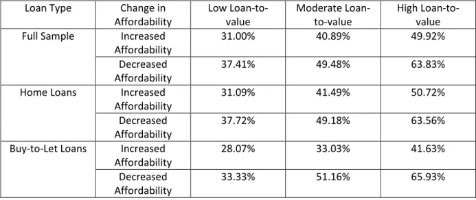
Table 7 follows on from Table 6a. We subdivide the loans into those that have undergone a decrease in a¤ordability since loan origination (for example due to unemployment, lower household income, or higher short-term debt obligations) and those have undergone an increase, and look at the default rates for the three levels of current loan-to-value, using the interquartile range for the middle loan-to-value category, as in Table 6. Both decreased a¤ordability and the current loan-to-value ratio have an impact on default rates, and the two e¤ects interact, as in Table 6.

six explanatory variables:

Prob(defaulti) = ( 0+ 1LTVi+ 2A¤ordi+ 3LogIncomei+

4AppLTVi+ 5AppA¤ordi+ 6AppLogIncomei

The results are shown in Table 8, for all loans in the database, and then for the subsample of home loans and buy-to-let loans estimated separately.

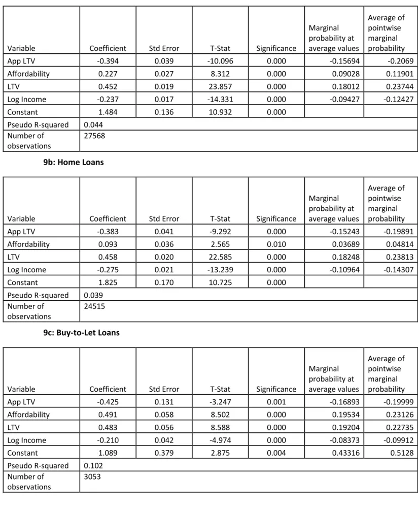
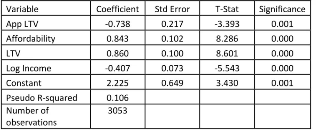
Application-date a¤ordability index and application-date log income have weak explanatory power in Table 8. In Table 9 we re-estimate the probit models dropping these two variables. In Table 10 we show estimates of this same model using the logistic distribution in place of the normal distribution. We will focus on the probit model with four explanatory variables (Table 9). The last two columns in Table 9 show the marginal impact on default probability of a marginal change in each explanatory variable, calculated two ways: using the sample average of the other explanatory variables, and computed individually at each sample point and then averaged across the sample. Both measures are used in the literature but the latter is generally considered preferable; see Green (2000). Current log income has more impact on the default decision than the current a¤ordability index. A strong and surprising …nding is the notable power of current loan-to-value in determining Irish mortgage default decisions, as measured by these marginal probabilities. This strong relative explanatory power is further increased by the fact that current loan-to-value has a wider interquartile range than the a¤ordability index and log income.

A key topic in the existing US research literature is measuring the pro-portion of mortgage defaulters which are distressed (inability to pay) versus strategic (put-optionality) defaults. The current loan-to-value ratio is the key variate in a strategic defaulter’s decision calculus, whereas loan-to-value has no role in a distressed defaulter’s decision calculus. The high explana-tory power of current loan-to-value is evidence of strategic decision-making playing at least a partial role (explicitly or subconsciously) by Irish mortgage defaulters. The evidence indicates that Irish mortgage defaulters in our sam-ple have mixed motives, in‡uenced simultaneously by stressed a¤ordability and put optionality. Any "pure" strategic defaulters, with no a¤ordability pressure and motivated solely by put-optionality, are more likely to be in the 30% or so of non-cooperating mortgage defaulters, who do not submit an SFS and are not in our sample.

Lastly, we use nonparametric and semiparametric methods to examine potential nonlinearity in the response of default to loan-to-value. We use

the Gaussian kernel throughout and set the bandwidth h using Silverman’s rule of thumb, h = (4 d2

3n)

1

5;where 2

d is the sample variance of observed

de-faults and n is the number of observations in the sample or subsample. We estimate over the range 0<LTV<3but note with caution that kernel meth-ods are unreliable in the tails of the data range. The 99% middle range of the data, leaving 0:5% in each tail of the sample, is (:06;2:62) for all loans,

(:02;2:28)for home loans, and(:17;3:07)for buy-to-let loans. Nonparametric or semiparametric estimates outside this middle range are untrustworthy.

Figure 2 shows unconditional expected default as a nonparametric func-tion of loan-to-value using kernel-based nonparametric regression; see equa-tion (5) in Secequa-tion 3.2. Figure 3 takes the nonparametrically-estimated ex-pected defaults from Figure 2 and compares them to the conditional exex-pected defaults from the probit model in Table 9; see equations (3) and (5) in Sec-tion 3.2. There is evidence for the type of nonlinearity predicted by opSec-tions theory in Figures 2 and 3, with the response curves ‡attening for LTV< 1

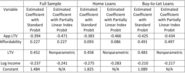
and curving upward at high LTV. Figure 4 shows the nonlinear LTV re-sponse functions estimated by the partially linear index probit model (see equation (7) in Section 3.2). The results are suggestive, but not de…nitive, regarding a convex nonlinearity in the link between loan-to-value and loan default; see Elul et al. (2010) for related evidence for the US market us-ing di¤erent estimation methods (step-wise linearity over intervals in a logit model). The convex nonlinearity, as re‡ected in a nonzero linear model bias, seems to start at a loan-to-value ratio of 1.5 for home loans. For buy-to-let mortgages, the convex nonlinearity starts earlier, near a loan-to-value ratio of 1.0. The coe¢ cient estimates for the other …ve variables (for which the linearity assumption is maintained) are shown in the supplementary tables in the appendix.

5

Conclusion

Following the collapse of the Irish credit/property bubble, Irish residential property prices fell sharply and mortgage arrears grew explosively. From the peak in Q2 2007, residential property prices fell 50.3% to the trough in Q2 2012, subsequently recovering 1.2% from the trough by Q2 2013. The number of home mortgages in default (greater than 90 days of accumulated arrears) grew 272.6%, from 26,271 in Q3 2009 to 97,874 in Q2 2013; as of Q2 2013, 12.7% of home loan mortgages are in default. Data on buy-to-let

defaults is only available recently so the growth path is not known, but 20.4% of buy-to-let mortgages are in default as of Q2 2013.

Property price falls have been shown to have a strong causal link to house-hold mortgage default decisions, in a wide range of studies using US data. Although property resale price has no e¤ect on a household’s ability to pay the mortgage, it has a large e¤ect on the implicit put-option value of mort-gage default. Unless the lender has unhindered recourse to the household’s future income, the holder of a negative equity mortgage can e¤ectively "put" the property to the lender and in exchange stop paying the mortgage. This put-optionality e¤ect on mortgage default has been shown to be particulary strong when combined with household income stress. In the "dual trigger" model of mortgage default, households are particularly likely to default when household income stress is combined with large positive put-option value of default, captured by a loan-to-value ratio substantially above 1.0.

This paper con…rms key US-data …ndings on recent Irish mortage data. We rely on a data set which only contains borrowers within the Mortgage Arrears Resolution Process who have submitted a Standard Financial State-ment, so non-cooperating borrowers, and borrowers who have never experi-enced mortgage di¢ culties, are censored from the data. Within this restricted set of borrowers, the loan-to-value ratio is a very important, arguably the most important, predictor of mortgage default. Our evidence supports the dual-trigger model of default: Irish mortgage borrowers are most likely to de-fault when income stress is combined with strong put-optionality as re‡ected in the loan-to-value ratio. The consensus view from US-based research is that both a¤ordability and put-optionality a¤ect default rates, but a¤ord-ability is the more important in‡uence. In our doubly-censored Irish sample, put-optionality is a more powerful predictor of default than a¤ordability.

References

[1] Asay, M. R., 1978, Rational mortgage pricing. Ph.D. diss. University of Southern California, Los Angeles. (Also in Research Paper in Banking and Financial Economics, No. 30, Board of Governors of the Federal Reserve System, 1979.)

[2] Bellemare, Charles, Bertrand Melenberg, and Arthur van Soest, 2002, Semi-parametric models for satisfaction with income, Portuguese Eco-nomic Journal 1, 2, 181-203.

[3] Bhutta, Neil, Jane Dokko, and Hui Shan, 2010, The depth of negative eq-uity and mortgage default decisions, working paper no 2010-35, Finance and Economics Discussion Series Divisions of Research & Statistics and Monetary A¤airs Federal Reserve Board, Washington, D.C.

[4] Burke, Jeremy, and Kata Mihaly, 2012, Financial literacy, social percep-tion and strategic default, working paper no WR-937, RAND Corpora-tion, Santa Monica, CA.

[5] Carroll, R. J., Jianqing Fan, Irene Gijbels, and M. P. Wand, 1997, Gen-eralized partially linear single-index models, Journal of the American Statistical Association 92, 438, 477-489.

[6] Cunningham, D. F., and P. H. Hendershott, 1984, Pricing FHA mort-gage default insurance, Housing Finance Review, 13, 373-392.

[7] Cutts, A.C., and W. A. Merrill, 2008, Interventions in mortgage default: Policies and practices to prevent home loss and lower costs, Freddie Mac Working Paper #08-01

[8] Deng, Yongheng, John M. Quigley, and Robert van Order, 2000, Mort-gage terminations, heterogeneity and the exercise of mortMort-gage options,

Econometrica 68, 2, 275-307.

[9] Elmer, Peter J., and Steven A. Seelig, 1999, Insolvency, trigger events, and consumer risk posture in the theory of single-family mortgage de-fault, Journal of Housing Research 10, 1, 1-25.

[10] Elul, Ronel, Nicholas S. Souleles, Souphala Chomsisengphet, Dennis Glennon, and Robert Hunt, 2010, What "triggers" mortgage default?,

American Economic Review 100, 2, 490-494.

[11] Epperson, James, James B. Kau, Donald Keenan and Walter Muller, 1985, Pricing default risk in mortgages, Journal of the American Real Estate and Urban Economics Association 13, 3, 261-272.

[12] Foote, Christopher, Kristopher Geraldi and Paul Willen, 2008, Neg-ative equity and foreclosure: theory and evidence, Journal of Urban Economics 64, 2, 234-245.

[13] Greene, William, 2000, Econometric Analysis, Pearson, London.

[14] Guiso, Luigi, Paola Sapienza and Luigi Zingales, 2009, Moral and social constraints to strategic default on mortgages, working paper no. 15145, National Bureau of Economic Research.

[15] Horowitz, Joel, and N. E. Savin, 2001, Binary response models: Logits, probits and semiparametrics, The Journal of Economic Perspectives 15, 4, 43-56.

[16] Härdle, Wolfgang, Sylvie Huet, Enno Mammen, and Stefan Sperlich, 2004, Bootstrap inference in semiparametric generalized additive mod-els, Econometric Theory 20, 2, 265-300.

[17] Luca, G. De, 2008, SNP and SML estimation of univariate and bivariate binary-choice models, Stata Journal 8, 2, 190-220.

[18] Lydon, R., and Y. McCarthy, 2011, What lies beneath: Understanding recent trends in Irish mortgage arrears, paper delivered at the Central Bank of Ireland conference on the Irish mortgage market in context, Dublin, Ireland, October 2011.

[19] Mac Coille, C., S. Lyons, D. McNamara and E. Lang, 2013, Ireland’s de-teriorating mortgage arrears crisis, Davy research report: Irish economy and the banks, July 2013.

[20] Matzkin, Rosa L., 1992, Nonparametric and distribution-free estimation of the binary threshold crossing and the binary choice models, Econo-metrica 60, 2, 239-270.

[21] Seiler, Michael, Vicky Seiler, Mark Lane and David Harrison, 2012, Fear, shame and guilt: economic and behavioral motivations for strategic default, Real Estate Economics, forthcoming.

[22] Severini, Thomas A., and Joan G. Staniswalis, 1994, Quasi-likelihood es-timation in semiparametric models, Journal of the American Statistical Association 89, 426, 501-511.

[23] Shen, Xiangjin, Shiliang Li, and Hiroki Tsurumi, 2013, Comparison of parametric and semi-parametric binary response models, working paper no 201308, Rutgers University, Department of Economics.

[24] Tirupattur, Vishwanath, Oliver Chang and James Egan, 2010, ABS market insights: understanding strategic defaults, Morgan Stanley Re-search Note.

[25] Towe, Charles and Chad Lawley, 2010, The contagion e¤ect of neighbor-ing foreclosures on own foreclosures, National Center for Smart Growth, University of Maryland.

[26] Trautmann, Stefan, and Razvan Vlahu, 2011, Strategic loan defaults and coordination: An experimental analysis, working paper no 312, Nether-lands Central Bank, Research Department.

[27] Wyman, Oliver, 2009, Understanding strategic defaults in mortgages, Experian-Oliver Wyman Market Intelligence Report 2009 Topical Re-port Series.

Technical Appendix

This technical appendix contains background material on the nonpara-metric regression estimation procedure presented in Section 3.2. First we assume that the default decision index is fully nonparametric:

vi =f(xi) +"i

and wish the estimate the univariate nonparametric relationship between x1i

and expected default. De…ne g(x1i) as conditional expected default:

g(x1i) =E[dijx1i] =E[ff(xi) +"ig+jx1i]

where _{f g}+ _{equals one if the argument is positive and otherwise zero. In} order to implement nonparametric kernel regression, we assume that g( ) is thrice continuously di¤erentiable. This imposes implicit assumptions on the smoothness of f( ) and on D; the multivariate distribution of x; we take this assumption as primitive, noting in passing that there are many explicit special cases off( )andDwhich would justify the assumption. Let idenote

the mean-zero deviation of realized default from conditional mean default:

di =g(x1i) + i

where we assume that the density function ofx1i is thrice continuously

di¤er-ential and that i has uniformly bounded conditional variance 2(x1i): Using

the Gaussian kernel together with bandwidth h = cn 15 to estimate bg(x_1i)

by (5), we have by Theorem 2.2 in Li and Racine (2007):

dlimpnh(_bg(x1i) g(x1i) b(x1i)) N(0;

2_(x 1i)

dens(x1i)

)

where b(x1i)is a standard bias correction term; see Li and Racine, page 62.

In the restricted case, we …rst estimate( 0; )under the assumption that the multivariate probit holds, and then nonparametrically estimate _bg(x1i)

using (6) applied to the predicted default rates from the estimated probit model. We ignore the estimation error in(b0;b)since it converges to zero at a faster rate than_bg(x1i) g(x1i):The same Theorem 2.2 from Li and Racine

Table 1: Percentage Distributions of Loan Type and Default Rates

All Loans Home

Loans Buy-to-Let Loans All Loans 100% 88.9% 11.1% % Loans in Default in

the Category 48.8% 48.7% 49.9%

Table 2: Statistical Distribution of Days in Arrears for Loan Accounts with

Nonzero Arrears

All Loans Home

Loans Buy-to-let Loans 10% Fractile 34 34 40.6 25% Fractile 110 106 150 Median 314 305 423 Mean 451.8 443.8 516.8 75% Fractile 662 642 766.3 90% Fractile 1037 1034 1095

Table 3: Data Distribution of Each Explanatory Variable Across Years of Loan

Origination

Net Income Payment-to-Income Ratio

Loan-to-Value Ratio Net Income 1999 or earlier 5.27% 3.72% 3.08% 5.27% 5.27% 5.15% 2000 2.55% 2.55% 2.17% 2.55% 2.55% 2.48% 2001 2.75% 2.74% 2.39% 2.75% 2.75% 2.68% 2002 3.65% 3.65% 3.22% 3.65% 3.65% 3.58% 2003 5.98% 5.98% 5.89% 5.98% 5.98% 5.84% 2004 8.76% 8.76% 8.75% 8.76% 8.76% 8.61% 2005 13.92% 13.92% 13.92% 13.92% 13.92% 13.67% 2006 21.30% 21.30% 21.29% 21.30% 21.30% 20.90% 2007 19.00% 19.00% 18.88% 19.00% 19.00% 18.58% 2008 13.22% 13.22% 12.87% 13.22% 13.22% 13.00% 2009 2.83% 2.83% 2.82% 2.83% 2.83% 2.77% 2010 0.53% 0.53% 0.52% 0.53% 0.53% 0.52% 2011 0.15% 0.15% 0.15% 0.15% 0.15% 0.15% 2012 0.07% 0.07% 0.06% 0.07% 0.07% 0.07% 2013 0.02% 0.00% 0.00% 0.02% 0.02% 0.02% Missing 13.68% 1.59% 3.98% 2.02% 0.00% 2.02% Truncated 0.11% 0.02% 0.00% 2.45% 0.41% 0.00%

Table 4: Descriptive Statistics of Explanatory Variables

Bottom

Quartile Median Top Quartile Mean Standard deviation Number of Observations Application Date Loan-to-Value .420 .640 .880 .631 .256 28061 Current Loan-to-Value .620 1.02 1.42 1.04 .570 28377 Application Date Payment-to-Income .290 .340 .370 .336 .141 25549 Current Payment-to-Income .280 .380 .540 .471 .351 27879 Application Date Net Income €2664 €3517 €4473 €3843 €3390 27725 Current Net Income €1802 €2529 €3480 €2840 €1868 27879

Table 5: Correlation Matrix of the Explanatory Variables

LTV Application

Date LTV Affordability Application Date Affordability

Log Income Application Date Log Income LTV 1.000 Application Date LTV 0.655 1.000 Affordability 0.113 0.039 1.000 Application Date Affordability 0.081 0.020 0.109 1.000 Log Income 0.076 0.012 -0.556 0.073 1.000 Application Date Log Income 0.123 0.096 0.014 0.012 0.164 1.000

Table 6: Default rates for loans doubly-sorted by loan-to-value,

payment-to-income and net payment-to-income: Full Sample

6a: Default rates for loans sorted by loan-to-value and affordability

Low Payment-to-_Income Moderate Payment-to-_Income High Payment-to-_Income

Low LTV 43.43% 39.04% 46.03%

Moderate LTV 41.55% 43.98% 57.34%

High LTV 47.40% 56.47% 70.55%

6b: Default rates for loans sorted by loan-to-value and net income

High Income Moderate Income Low Income

Low LTV 31.91% 40.26% 48.85%

Moderate LTV 39.11% 47.40% 56.63%

High LTV 51.34% 59.78% 69.13%

6c: Default rates for loans sorted by affordability and net income

High Income Moderate _Income Low Income Low Payment-to-Income 38.40% 42.02% 51.39% Moderate

Payment-to-Income 45.11% 47.31% 60.27%

Table 7: Proportions of Loans in Default for Subcategory of Loan-to-value and

Increased/Decreased Affordability

Loan Type Change in

Affordability Low Loan-to-value Moderate Loan-to-value High Loan-to-value Full Sample Increased

Affordability 31.00% 40.89% 49.92% Decreased

Affordability 37.41% 49.48% 63.83% Home Loans Increased

Affordability 31.09% 41.49% 50.72% Decreased

Affordability 37.72% 49.18% 63.56% Buy-to-Let Loans Increased

Affordability 28.07% 33.03% 41.63% Decreased

Table 8: Probit Model of Default with Six Explanatory Variables

8a: Full Sample

Variable Coefficient Std Error T-Stat Significance App Affordability -0.063 0.058 -1.081 0.280 App LTV -0.617 0.043 -14.261 0.000 App Log Income 0.016 0.011 1.471 0.141 Affordability 0.312 0.031 10.170 0.000 LTV 0.620 0.022 28.443 0.000 Log Income -0.192 0.019 -10.310 0.000 Constant 0.901 0.159 5.664 0.000 Pseudo R-squared 0.059 Number of observations 25116 8b: Home Loans

Variable Coefficient Std Error T-Stat Significance App Affordability -0.078 0.066 -1.184 0.236 App LTV -0.619 0.046 -13.531 0.000 App Log Income 0.019 0.021 0.895 0.371 Affordability 0.225 0.043 5.274 0.000 LTV 0.628 0.023 26.865 0.000 Log Income -0.207 0.026 -7.965 0.000 Constant 1.024 0.197 5.200 0.000 Pseudo R-squared 0.054 Number of observations 22474 8c: Buy-to-Let Loans

Variable Coefficient Std Error T-Stat Significance App Affordability 0.043 0.135 0.318 0.750 App LTV -0.564 0.143 -3.930 0.000 App Log Income 0.021 0.013 1.663 0.096 Affordability 0.551 0.068 8.132 0.000 LTV 0.578 0.063 9.135 0.000 Log Income -0.205 0.048 -4.222 0.000 Constant 0.772 0.438 1.763 0.078 Pseudo R-squared 0.115 Number of observations 2642

Table 9: Probit Model of Default with Four Explanatory Variables

9a: Full Sample

Variable Coefficient Std Error T-Stat Significance

Marginal probability at average values Average of pointwise marginal probability App LTV -0.394 0.039 -10.096 0.000 -0.15694 -0.2069 Affordability 0.227 0.027 8.312 0.000 0.09028 0.11901 LTV 0.452 0.019 23.857 0.000 0.18012 0.23744 Log Income -0.237 0.017 -14.331 0.000 -0.09427 -0.12427 Constant 1.484 0.136 10.932 0.000 Pseudo R-squared 0.044 Number of observations 27568 9b: Home Loans

Variable Coefficient Std Error T-Stat Significance

Marginal probability at average values Average of pointwise marginal probability App LTV -0.383 0.041 -9.292 0.000 -0.15243 -0.19891 Affordability 0.093 0.036 2.565 0.010 0.03689 0.04814 LTV 0.458 0.020 22.585 0.000 0.18248 0.23813 Log Income -0.275 0.021 -13.239 0.000 -0.10964 -0.14307 Constant 1.825 0.170 10.725 0.000 Pseudo R-squared 0.039 Number of observations 24515 9c: Buy-to-Let Loans

Variable Coefficient Std Error T-Stat Significance

Marginal probability at average values Average of pointwise marginal probability App LTV -0.425 0.131 -3.247 0.001 -0.16893 -0.19999 Affordability 0.491 0.058 8.502 0.000 0.19534 0.23126 LTV 0.483 0.056 8.588 0.000 0.19204 0.22735 Log Income -0.210 0.042 -4.974 0.000 -0.08373 -0.09912 Constant 1.089 0.379 2.875 0.004 0.43316 0.5128 Pseudo R-squared 0.102 Number of 3053

Table 10: Logit Model of Default with Four Explanatory Variables

10a: Full Sample

Variable Coefficient Std Error T-Stat Significance App LTV -0.724 0.066 -10.954 0.000 Affordability 0.361 0.046 7.875 0.000 LTV 0.797 0.034 23.335 0.000 Log Income -0.406 0.027 -14.922 0.000 Constant 2.572 0.223 11.545 0.000 Pseudo R-squared 0.046 Number of observations 27568 10b: Home Loans

Variable Coefficient Std Error T-Stat Significance App LTV -0.712 0.070 -10.193 0.000 Affordability 0.125 0.060 2.085 0.037 LTV 0.811 0.037 22.069 0.000 Log Income -0.467 0.034 -13.703 0.000 Constant 3.123 0.279 11.211 0.000 Pseudo R-squared 0.040 Number of observations 24515 10c: Buy-to-Let Loans

Variable Coefficient Std Error T-Stat Significance App LTV -0.738 0.217 -3.393 0.001 Affordability 0.843 0.102 8.286 0.000 LTV 0.860 0.100 8.601 0.000 Log Income -0.407 0.073 -5.543 0.000 Constant 2.225 0.649 3.430 0.001 Pseudo R-squared 0.106 Number of observations 3053

Tables Appendix

Table A.1: Default rates for loans doubly-sorted by loan-to-value,

payment-to-income and net income: Home loans

A.1.a: Default rates for loans sorted by loan-to-value and affordability

Low Payment-to-_Income Moderate Payment-to-_Income High Payment-to-_Income

Low LTV 43.70% 39.44% 45.77%

Moderate LTV 42.70% 44.57% 56.97%

High LTV 48.40% 56.84% 70.69%

A.1.b: Default rates for loans sorted by loan-to-value and net income

High Income Moderate Income Low Income

Low LTV 32.70% 40.11% 48.63%

Moderate LTV 38.67% 46.83% 55.69%

High LTV 51.08% 59.41% 67.97%

A.1.c: Default rates for loans sorted by affordability and net income

High Income Moderate Income Low Income Low Payment-to-Income 39.37% 43.08% 45.69% Moderate

Payment-to-Income 45.28% 47.43% 59.59%

Table A.2: Default rates for loans doubly-sorted by loan-to-value,

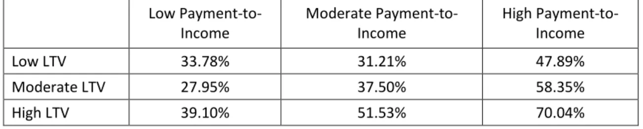
payment-to-income and net income: Buy-to-let loans

A.2.a: Default rates for loans sorted by loan-to-value and affordability

Low Payment-to-_Income Moderate Payment-to-_Income High Payment-to-_Income

Low LTV 33.78% 31.21% 47.89%

Moderate LTV 27.95% 37.50% 58.35%

High LTV 39.10% 51.53% 70.04%

A.2.b: Default rates for loans sorted by loan-to-value and net income

High Income Moderate Income Low Income

Low LTV 27.49% 43.90% 57.14%

Moderate LTV 40.29% 53.44% 69.85%

High LTV 52.15% 64.78% 85.00%

A.2.c: Default rates for loans sorted by affordability and net income

High Income Moderate Income Low Income Low Payment-to-Income 31.44% 38.29% 53.08% Moderate

Payment-to-Income 36.07% 43.94% 62.06%

Table A.3: Partially-linear Index Probit Model of Default with Four

Explanatory Variables

Full Sample Home Loans Buy-to-Let Loans

Variable Estimated Coefficient with Standard Probit Estimated Coefficient with Partially Linear Index Probit Estimated Coefficient with Standard Probit Estimated Coefficient with Partially Linear Index Probit Estimated Coefficient with Standard Probit Estimated Coefficient with Partially Linear Index Probit App LTV -0.394 -0.471 -0.383 -0.466 -0.425 -0.434 Affordability 0.227 0.227 0.093 0.086 0.491 0.497

LTV 0.452 Nonparametric 0.458 Nonparametric 0.483 Nonparametric Log Income -0.237 -0.241 -0.275 -0.283 -0.210 -0.217

0 50 100 150 200 250 300 350 400

Figure 1: Comparative Time Series of Irish Residential Property Price Index, Unemployment Rate, Per-capital Real Income and Home Loan

Default Rate

0 0.1 0.2 0.3 0.4 0.5 0.6 0.7 0.8 0.9 1 0 0.25 0.5 0.75 1 1.25 1.5 1.75 2 2.25 2.5 2.75 3

Figure 2: Local Proportion of Loans in Default as a Function of Loan-to-Value All Loans Home Loans BTL

-0.2 0 0.2 0.4 0.6 0.8 1 0 0.5 1 1.5 2 2.5 3

Figure 3a: Restricted and Unrestricted Nonparametric Estimation of the Probability of Default as a Function of Loan-to-Value, All Loans

Local Proportion of Defaults Explained Probability of Default Using Multivariable Probit

-0.2 0 0.2 0.4 0.6 0.8 1 0 0.5 1 1.5 2 2.5 3

Figure 3b: Restricted and Unrestricted Nonparametric Estimation of the Probability of Default as a Function of Loan-to-Value, Home Loans

Local Proportion of Defaults Explained Probability of Default Using Multivariable Probit Linear Model Bias

-0.2 0 0.2 0.4 0.6 0.8 1 0 0.5 1 1.5 2 2.5 3

Figure 3c: Restricted and Unrestricted Nonparametric Estimation of the Probability of Default as a Function of Loan-to-Value, BTL Loans

Local Proportion of Defaults Explained Probability of Default Using Multivariable Probit

-0.5 0 0.5 1 1.5 2 2.5 3 0 0.5 1 1.5 2 2.5 3

Figure 4a: Linear and Semiparametric Estimates of the Contribution of Loan-to-Value to the Default Decision Index, All Loans

Semiparametric Estimate Linear Estimate

-1 0 1 2 3 4 5 0 0.5 1 1.5 2 2.5 3

Figure 4b: Linear and Semiparametric Estimates of the Contribution of Loan-to-Value to the Default Decision Index, Home Loans

Semiparametric Estimate Linear Estimate

-0.5 0 0.5 1 1.5 2 0 0.5 1 1.5 2 2.5 3

Figure 4c: Linear and Semiparametric Estimates of the Contribution of Loan-to-Value to the Default Decision Index, Buy-to-Let Loans

Semiparametric Estimate Linear Estimate