CIRJE Discussion Papers can be downloaded without charge from: http://www.e.u-tokyo.ac.jp/cirje/research/03research02dp.html
Discussion Papers are a series of manuscripts in their draft form. They are not intended for circulation or distribution except as indicated by the author. For that reason Discussion Papers may not be reproduced or distributed without the written consent of the author.
CIRJE-F-745
Pricing Barrier and Average Options
under Stochastic Volatility Environment
Kenichiro Shiraya
Graduate School of Economics, University of Tokyo and Mizuho-DL Financial Technology Co., Ltd.
Akihiko Takahashi University of Tokyo
Masashi Toda
Graduate School of Economics, University of Tokyo May 2010
Pricing Barrier and Average Options
under Stochastic Volatility Environment
1
Kenichiro Shiraya
2,
Graduate School of Economics, the University of Tokyo, Mizuho-DL Financial Technology Co., Ltd.
Akihiko Takahashi
3Graduate School of Economics, the University of Tokyo 7-3-1, Hongo, Bunkyo-ku, Tokyo, 113-0033, Japan.
and
Masashi Toda
4Graduate School of Economics, the University of Tokyo 7-3-1, Hongo, Bunkyo-ku, Tokyo, 113-0033, Japan.
First Version: October 27, 2009, Current Version: May 12, 2010
1We are very grateful to anonymous referees and the editor, Professor Peter Forsyth for their efforts and precious
comments that improve the previous version substantially.
2Tel: 81-3-5219-2396, e-mail: kenichiro-shiraya@fintec.co.jp. The views expressed in this paper are those of the
author and do not necessarily represent the views of Mizuho-DL Financial Technology Co., Ltd.
3Tel: 81-3-3812-2111, e-mail: [email protected]. 4
Abstract
This paper proposes a new approximation method of pricing barrier and average options under stochastic volatility environment by applying an asymptotic expansion approach. In particular, a high-order expansion scheme for general multi-dimensional diffusion processes is effectively applied. Moreover, the paper com-bines a static hedging method with the asymptotic expansion method for pricing barrier options. Finally, numerical examples show that the fourth or fifth-order asymptotic expansion scheme provides sufficiently accurate approximations under theλ-SABR and SABR models.
Keywords: barrier option, average option, knock-out option, stochastic volatility, static hedge, asymp-totic expansion,λ-SABR model, SABR model
1
Introduction
Recently, it is a necessary and important task to evaluate exotic options such as barrier and average options based on calibration to liquid plain-vanilla option prices. Pricing vanilla options under some stochastic volatility model is a typical approach to calibration. However, to our knowledge closed-form solutions for exotic options’ prices under stochastic volatility models are rarely obtained and hence pricing should usually rely on numerical approximation methods such as Monte Carlo methods or finite difference/element methods. For example, Itkin and Carr [17] solved barrier options using a PDE method and Ninomiya-Victoir [28] computed an average option using a Monte Carlo method. Straightforward application of those methods are time-consuming or/and produces only inaccurate estimates. Thus, we need to develop some sophisticated technique with those methods to satisfy requirements in practice. Alternatively, if we can obtain a closed-form formula that creates an accurate and fast-computing approximation, it is very useful. This paper proposes an approximation method of pricing barrier and average options under stochastic volatility environment by applying an asymptotic expansion approach. In particular, a high-order expansion scheme for general multi-dimensional diffusion processes recently developed by Takahashi-Takehara-Toda [36] is effectively applied. Moreover, for pricing barrier options the paper combines the asymptotic ex-pansion method with a static hedging method by Fink [9]. Numerical examples show that the fourth or fifth-order approximation of an asymptotic expansion scheme provides sufficiently fast and accurate ap-proximations in practice under theλ-SABR model(Labordere [21]) and the SABR model(Hagan et.al. [15]); our method gives good approximations even in high volatility or/and high volatility on volatility situations, when it is usually difficult for numerical approximations to produce fast and accurate approximations.
For over a decade, static hedging techniques have been developed and investigated extensively for barrier type options. Bowie and Carr [2] and Carr, Ellis and Gupta [6] consider a static hedge method for barrier-type and lookback options by usingput call symmetry (Carr [3]). Derman, Ergener and Kani [8] proposes thecalendar-spreadsmethod. Carr and Picron [7] presents a method for static hedging of timing risk which is applied to pricing barrier options. Carr and Chou [4], [5] shows a representation of any twice differentiable payoff function and then develops the so called strike-spreadsmethod for static hedging of barrier, ratchet and lookback options under the Black-Scholes model.
Fink [9] generalizes the method of Derman, Ergener and Kani [8] for barrier options in a Heston’s stochastic volatility. More recently, Nalholm and Poulsen [26] proposes a new technique for static hedging of barrier options under general asset dynamics, such as a jump-diffusion process with correlated stochastic volatility. Furthermore, Nalholm and Poulsen [25] examines the sensitivity of dynamic and static hedging methods for barrier options to model risk.
The asymptotic expansion is first applied to finance for evaluation of an average option that is a popular derivative in commodity markets. Kunitomo and Takahashi [18] and Takahashi [30] derive the approxi-mation formulas for an average option by an asymptotic method based on log-normal approxiapproxi-mations of an average price distribution when the underlying asset price follows a geometric Brownian motion(under the Black-Scholes model). Yoshida [42] applies a formula derived by the asymptotic expansion of certain statistical estimators for small diffusion processes. Thereafter, the asymptotic expansion have been ap-plied to a broad class of problems in finance: See Takahashi [31], [32], Kunitomo and Takahashi [19], [20], Matsuoka, Takahashi and Uchida [23], Takahashi and Yoshida [37], [38], Muroi [24], and Takahashi and Takehara [33], [34], [35].
Although the asymptotic expansion method is applied to average options in [42], [30], [31], this paper is the first one that implements the expansion more than the second order and examines its numerical accuracy under stochastic volatility environment.
Moreover, to our best knowledge, other closed-form (approximation) formulas for barrier or average options under stochastic volatility environment have not been shown except Fouque, Papanicolaou and Sircar [10], [11] and Fouque and Han [12], [13]. They apply the singular perturbation method to pricing Barrier and Asian(average) options in a fast mean-reverting stochastic volatility model. See Yamamoto and Takahashi [40] for the accuracy of the approximation method; it shows through numerical experiments that the method provides sufficiently accurate option prices in a fast mean-reversion case of the volatility process while it does not in a non-fast mean-reversion case.
The organization of the paper is as follows: After a brief explanation of the asymptotic expansion in the next section, Section 3 introduces a new computation algorithm for the asymptotic expansion and derives an
approximation formula for a density function of the underlying asset. Section 4 proposes an approximation method for pricing barrier options under stochastic volatility models by applying the asymptotic expansion with a static hedging method. It also provides numerical examples under theλ-SABR model. Section 5 applies the high-order expansion scheme to pricing average options and presents numerical examples under the SABR andλ-SABR models. Section 6 concludes. Finally, some error analysis is given in Appendix.
2
An Asymptotic Expansion in a Multi-dimensional Diffusion
Process
This section briefly describes an asymptotic expansion method in a general multi-dimensional diffusion process. See Section 2 of [36] for the details.
Let (W, P) be the r-dimensional Wiener space. We consider ad-dimensional diffusion process Xt(ϵ) = (Xt(ϵ),1,· · ·, Xt(ϵ),d) which is the solution to the following stochastic differential equation:
dXt(ϵ),i=V0i(Xt(ϵ), ϵ)dt+ϵVi(Xt(ϵ))dWt (i= 1,· · ·, d) (1)
X0(ϵ)=x0∈Rd
whereW = (W1,· · ·, Wr) is ar-dimensional standard Wiener process, andϵ∈(0,1] is a known parameter.
Suppose thatV0= (V01,· · ·, V0d) :Rd×(0,1]7→RdandV = (V1,· · ·, Vd): Rd7→Rd⊗Rrsatisfy some regularity conditions.(e.g. V0 andV are smooth functions with bounded derivatives of all orders.)
Next, suppose that a function g : Rd 7→R to be smooth and all derivatives have polynomial growth
orders. Then, a smooth Wiener functionalg(XT(ϵ)) has its asymptotic expansion;
g(XT(ϵ))≈g0T +ϵg1T +· · ·
inLp for everyp >1(or inD∞) asϵ↓0. The coefficients in the expansiongnT ∈D∞(n= 0,1,· · ·) can be
obtained by Taylor’s formula and represented based on multiple Wiener-Itˆo integrals. Here,D∞ denotes the set of smooth Wiener functionals. See chapter V of Ikeda and Watanabe [16] for the detail.
Note that the leading term of the expansiong0T is deterministic and expressed as
g0T =g(X
(0)
T ),
whereXt(0)= (Xt(0),1,· · ·, Xt(0),d) is the solution of the ordinary differential equation:
dXt(0),i=V0i(Xt(0),0)dt (i= 1,· · ·, d) (2) X0(0)=x0∈Rd. Next, normalizeg(XT(ϵ)) to G(ϵ)= g(X (ϵ) T )−g0T ϵ forϵ∈(0,1]. Then, G(ϵ)≈g1T+ϵg2T +· · ·
inLpfor every p >1(or inD∞). Moreover, let
ˆ
V(x, t) = (∂g(x))′[YTYt−1V(x)]
whereY denotes the solution to the differential equation;
dYt=∂V0(X
(0)
t ,0)Ytdt; Y0=Id.
Here, ∂V0 denotes thed×dmatrix whose (j, k)-element is∂kV0j=
∂V0j(x,ϵ)
∂xk ,V
j
0 is thej-th element ofV0, andId denotes thed×didentity matrix.
Further, we make the following assumption: (Assumption 1) ΣT = ∫ T 0 ˆ V(Xt(0), t) ˆV(Xt(0), t)′dt >0.
Note that g1T follows a normal distribution with variance ΣT; the density function of g1T denoted by
fg1T(x) is given by fg1T(x) = 1 √ 2πΣT exp ( −(x−C)2 2ΣT ) where C= (∂g(XT(0)))′ ∫ T 0 YTYt−1∂ϵV0(X (0) t ,0)dt.
Hence, Assumption 1 means that the distribution ofg1T does not degenerate. In application, it is easy to
check this condition in most cases.
LetSbe the real Schwartz space of rapidly decreasingC∞-functions onRandS′be its dual space that is the space of the Schwartz tempered distributions. Next, take Φ∈ S′. Then, by Watanabe theory(Watanabe [39], Yoshida [41]) a generalized Wiener functional Φ(G(ϵ)) has an asymptotic expansion inD−∞ asϵ↓0 whereD−∞ denotes the set of generalized Wiener functionals. See chapter V of Ikeda and Watanabe [16] for the detail. Hence, the expectation of Φ(G(ϵ)) is expanded around ϵ= 0 as follows: ForN = 0,1,2,· · ·,
E[Φ(G(ϵ))] = N ∑ j=0 ϵj j ∑ m=0 1 m! ∫ R Φ(x) ∑ k∈Kj,m Cj,m,k(−1)m ∂ m ∂xm{E [ Xj,m,kg1T =x ] fg1T(x)}dx+o(ϵ N) (3) where Φ(m)(g1T) = ∂mΦ(x) ∂xm x=g1T , (4) Kj,m = { (k1,· · ·, kj−m+1);kn≥0, j−∑m+1 n=1 kn=m, j−∑m+1 n=1 nkn=j } , (5) Xj,m,k = j−∏m+1 n=1 gkn (n+1)T, (6) Cj,m,k = j−∏m+1 n=1 m! k1!· · ·kj−m+1! . (7)
3
General Computational Scheme of Asymptotic Expansion
This section explains a general computational scheme of the asymptotic expansion developed by [36]. See Section 4 of [36] for the details. First, to compute conditional expectations E[Xj,m,kg
1T =x
]
in the right hand side of (3) we introduce the following lemma which can be derived from a property of Hermite polynomials and leads us to compute the unconditional expectations instead of the conditional ones. Lemma 1 Let (Ω, F, P) be a probability space. Suppose that X ∈ L2(Ω, P) andZ is a random variable with Gaussian distribution with mean 0 and variance Σ. Then, the conditional expectation E[X|Z = x] has the following expansion in L2(R, µ)whereµis the Gaussian measure onRwith mean0 and variance Σ: E[X|Z=x] = ∞ ∑ n=0 anHn(x; Σ) (8)
whereHn(x; Σ) is the Hermite polynomial of degreenwhich is defined as
Hn(x; Σ) = (−Σ)nex 2/2Σ dn
dxne
and coefficientsan are given by an = 1 n! 1 (iΣ)n ∂n ∂ξn ξ=0 { eξ 2 2ΣE[eiξZX] } . (9)
(proof )See Lemma 4 of [36]. Here we define ˆg1T as ˆ g1T = (∂g(X (0) T )) ′∫ T 0 [YTYt−1V(X (0) t )]dWt=g1T −C, and define ZT⟨ξ⟩= exp{iξˆg1T+ ξ2 2 ΣT}.
Then, from Lemma 1 and (3), we have the following expression ofE[Φ(G(ϵ))]:
E[Φ(G(ϵ))] = N ∑ j=0 ϵj j ∑ m=0 1 m! ∫ R Φ(x) ∑ k∈Kj,m Cj,m,k(−1)m ∂ m ∂xm{ j∑+m l=0 aj,m,kl Hl(x−C; ΣT)fg1T(x)}dx+o(ϵ N) where aj,m,kl = 1 l! 1 (iΣT)l ∂l ∂ξl ξ=0 { E[Xj,m,kZT⟨ξ⟩] } .
In particular, let Φ be the delta function atx∈R, δx, we obtain the asymptotic expansion of density
ofG(ϵ): fG(ϵ)(x) = E[δx(G(ϵ))] = N ∑ j=0 ϵj j ∑ m=0 ∑ k∈Kj,m j∑+m l=0 aj,m,kl Cj,m,k m! (−1) m ∂ m ∂xm{Hl(x−C; ΣT)fg1T(x)}+o(ϵ N). (10)
3.1
Asymptotic Expansion of Density Function
This subsection summarizes a general computational method for the asymptotic expansion of the density function (10) developed by [36]. In particular, we show that coefficients in the expansion is obtained through a system of ordinary differential equations that is solved easily, and derive a concrete expression of the expansion up to ϵ2-order. Due to limitation of space, some equations necessary for the concrete expression of the expansion are omitted. See Section 4.1 of [36] for the full expressions.
First, the equation (10) is wrote down more explicitly up toϵ2-order:
fG(ϵ)(x) = a 0,0,(0) 0 H0(x−C; ΣT)fg1T(x) +ϵ { 2 ∑ l=0 a1l,1,(1)(−1) ∂ ∂x{Hl(x−C; ΣT)fg1T(x)} } +ϵ2 { 3 ∑ l=0 a2l,1,(0,1)(−1) ∂ ∂x{Hl(x−C; ΣT)fg1T(x)} +1 2 4 ∑ l=0 a2l,2,(2,0) ∂ 2 ∂x2{Hl(x−C; ΣT)fg1T(x)} } +o(ϵ2),
where coefficientsaj,m,kl are given by
a0l,0,(0) = 1 l! 1 (iΣT)l ∂l ∂ξl ξ=0 { E[ZT⟨ξ⟩] }
a1l,1,(1) = 1 l! 1 (iΣT)l ∂l ∂ξl ξ=0 { E[g2TZ⟨ ξ⟩ T ] } a2l,1,(0,1) = 1 l! 1 (iΣT)l ∂l ∂ξl ξ=0 { E[g3TZ⟨ ξ⟩ T ] } a2l,2,(2,0) = 1 l! 1 (iΣT)l ∂l ∂ξl ξ=0 { E[g22TZT⟨ξ⟩] } (11) To compute the unconditional expectations in (11), they derive ordinary differential equations (ODEs) of the components of the expectations.
We summarize the result of [36] as the following theorem (in the followings, for simplicity, it is assumed thatV0doesn’t depend onϵ, and writeV0(x, ϵ) asV0(x)) : See Section 4.1 of [36] for the details of derivation and the full expressions.
Theorem 1 The asymptotic expansion of the density of G(ϵ) up toϵ2-order is given by
fG(ϵ)(x) =fg1T(x) +ϵ { 3 ∑ l=1 C1lHl(x; ΣT) } fg1T(x) +ϵ 2 { 6 ∑ l=1 C2lHl(x; ΣT) } fg1T(x) +o(ϵ 2). where C1l= ΣTa 1,1,(1) l−1 , C21= ΣTa 2,1,(0,1) 0 , C2l= ΣTa 2,1,(0,1) l−1 + 1 2Σ 2 Ta 2,2,(2,0) l−2 (l≥2).
aj,m,kl are given by (11), and expectations in (11) are obtained as
E[g2TZ⟨ ξ⟩ T ] = 1 2 d ∑ i,j=1 ∂i∂jg(X (0) T )η i,j 2,2(t;ξ) + 1 2 d ∑ i=1 ∂ig(X (0) T )η i 2,1(t;ξ) E[g3TZ⟨ ξ⟩ T ] = 1 6 d ∑ i,j,k=1 ∂i∂j∂kg(X (0) T )η i,j,k 3,3 (t;ξ) + 1 2 d ∑ i,j=1 ∂i∂jg(X (0) T )η i,j 3,2(t;ξ) +1 6 d ∑ i=1 ∂ig(X (0) T )E[A i 3TZ⟨ ξ⟩ T ], E[g22TZT⟨ξ⟩] = 1 4 d ∑ i,j,k,l=1 ∂i∂jg(X (0) T )∂k∂lg(X (0) T )η i,j,k,l 4,4 (t;ξ) +1 2 d ∑ i,j,k=1 ∂i∂jg(X (0) T )∂ig(X (0) T )η i,j,k 4,3 (t;ξ) +1 4 d ∑ i,j=1 ∂ig(X (0) T )∂jg(X (0) T )η i,j 4,2(t;ξ)
whereηj,m are obtained as the solutions to the following system of ODEs:
d dtη j 1,1(t;ξ) = (iξ) ˆV(X (0) t , t)V j(X(0) t )′+ d ∑ j′=1 η1j′,1(t;ξ)∂j′V0j(Xt(0)) d dtη j 2,1(t;ξ) = 2(iξ) d ∑ j′=1 η1j′,1(t;ξ) ˆV(Xt(0), t)∂j′Vj(X (0) t )′ + d ∑ j′=1 η2j′,1(t;ξ)∂j′V0j(X (0) t ) + d ∑ j′=1 d ∑ k′=1 η2j′,,k2′(t;ξ)∂j′∂k′V0j(X (0) t )
d dtη j,k 2,2(t;ξ) = (iξ) { η1k,1(t;ξ) ˆV(Xt(0), t)Vj(Xt(0))′+η1j,1(t;ξ) ˆV(Xt(0), t)Vk(Xt(0))′ } +Vj(Xt(0))Vk(X (0) t )′+ d ∑ j′=1 d ∑ k′=1 ηj2,′2,k′(t;ξ)∂j′V0j(X (0) t )∂k′V0k(X (0) t ). (12)
Due to limitation of space, the remaining equations are omitted. See Proposition 2 in Section 4.1 of [36] for the full expressions.
Note that each ODE in (12) does not involve any higher order terms, and only lower or the same order terms appear in the right hand side of the ODE. So, one can easily solve (analytically or numerically) the system of ODEs and evaluate expectations. Indeed, for example, consider the following two-dimensional diffusion process with parameterϵ∈(0,1] which is known asλ-SABR Model(e.g. Labordere [21]):
dSt(ϵ) = µSt(ϵ)dt+ϵσt(ϵ)(S(tϵ))βdWt1, (13) dσ(tϵ) = λ(θ−σ(tϵ))dt+ϵν1σ (ϵ) t dW 1 t +ϵν2σ (ϵ) t dW 2 t.
Here, β ∈ [0,1] is a constant, W = (W1, W2) is a two dimensional Brownian motion and ν
1 = ρν,
ν2= (
√
1−ρ2)ν whereν is a positive constant andρ∈[−1,1].
To compute an option price on S, we need the density function of S whose asymptotic expansion is given by (10) with setting g(S, σ) = S. Then the corresponding differential equations up to the second order are given by
d dtη S 1,1(t;ξ) = (iξ)(S (0) t ) 2β(σ(0) t ) 2+µηS 1,1(t;ξ), d dtη σ 1,1(t;ξ) = (iξ)ν1(S (0) t ) β(σ(0) t ) 2−λησ 1,1(t;ξ), d dtη S 2,1(t;ξ) = 2(iξ)β(S (0) t ) 2β−1(σ(0) t ) 2ηS 1,1(t;ξ) + 2(iξ)(S (0) t ) 2βσ(0) t η σ 1,1(t;ξ) +µη S 2,1(t;ξ), where St(0) =S0eµt and σ (0)
t =e−λt(σ0−θ) +θ. Since these equations are linear and have hierarchical structure, one can easily integrate them as
η1S,1(t;ξ) = (iξ) ∫ t 0 eµ(t−t1)(St(0)1 ) 2β(σ(0) t1 ) 2dt 1, η1σ,1(t;ξ) = (iξ) ∫ t 0 e−λ(t−t1)ν 1(S (0) t1 ) β(σ(0) t1 ) 2dt 1, η2S,1(t;ξ) = 2(iξ)2 ∫ t 0 ∫ t1 0 eµ(t−t2)β(St1(0))2β−1(σt1(0))2(St2(0))2β(σ(0)t2 )2dt2dt1 +2(iξ)2 ∫ t 0 ∫ t1 0 eµ(t−t1)−λ(t1−t2)(St(0)1 ) 2βσ(0) t1 ν1(S (0) t2 ) β(σ(0) t2 ) 2dt 2dt1.
Integrals appeared in the right hand side can be analytically evaluated, but the expressions are lengthy and hence omitted. Other higher order terms can be easily integrated in the similar manner.
Then, the asymptotic expansion of the density function ofG(ϵ)= ST(ϵ)−S
(0) T ϵ can be expressed as fG(ϵ)(x)≈fg1T(x) +ϵC13H3(x; ΣT)fg1T(x) +· · · (14) where fg1T(x) = 1 √ 2πΣT exp ( − x2 2ΣT ) with ΣT = ∫ T 0 e2µ(T−t)(St(0))2β(σt(0))2dt
and C13 = 1 Σ3 T ∫ T 0 ∫ t1 0 eµ(T−t2)β(St1(0))2β−1(σt1(0))2(St2(0))2β(σt2(0))2dt2dt1 + 1 Σ3 T ∫ T 0 ∫ t1 0 eµ(T−t1)−λ(t1−t2)(S(0) t1 ) 2βσ(0) t1 ν1(S (0) t2 ) β(σ(0) t2 ) 2dt 2dt1.
Note that, since the first term of the expansion (14) is a normal density function, we can see that the asymptotic expansion method approximates the density function by a normal density function and its correction terms.
Moreover, we can provide some interpretations to the corrected terms of the expansion as follows: The
ϵ-order adjusts the approximated distribution partially to the skewness of implied volatilities because in the coefficient ofϵ, the correlation parameterρbetween the underlying asset price and its volatility appears for the first time. This is observed in Equation (13) whereC13includesν1=ρν. Also, theϵ2-order adjusts the approximated distribution partially to the smile, that is a fat tail of the true distribution of the asset price because full parameters of volatility on volatility (both ν1 and ν2) appear in the coefficient of ϵ2, though the equation is not reported in the paper due to its lengthy expression.
3.2
Asymptotic Expansion of Option Prices
This subsection applies the asymptotic expansion to option pricing. We consider the plain vanilla option on the underlying assetg(XT(ϵ)) whose dynamics is given by (1).
For example, an asymptotic expansion up to ϵ(N+1) of a call option price at time 0 with maturityT and strike priceK whereK=g(XT(0))−ϵy for arbitraryy∈Ris given by
C(K, T) = ϵP(0, T)
∫ ∞ −y
(x+y)fG(ϵ),N(x)dx+o(ϵ(N+1)).
Here,P(0, T) denotes the price at time 0 of a zero coupon bond with maturityT andfG(ϵ),N is the normal
asymptotic expansion of density ofG(ϵ) up toϵN-th order given by (10):
fG(ϵ),N(x) = N ∑ j=0 ϵj j ∑ m=0 ∑ k∈Kj,m j∑+m l=0 aj,m,kl Cj,m,k m! (−1) m ∂m ∂xm{Hl(x−C; ΣT)fg1T(x)}.
In particular, by Theorem 1, an asymptotic expansion up toϵ3of a call option price at time 0 with maturity
T and strike priceK whereK=g(XT(0))−ϵy for arbitraryy∈Ris expressed as
C(K, T) = ϵP(0, T) ∫ ∞ −y (x+y)fg1T(x)dx +ϵ2P(0, T) ∫ ∞ −y (x+y) { 3 ∑ l=1 C1lHl(x; ΣT) } fg1T(x)dx +ϵ3P(0, T) ∫ ∞ −y (x+y) { 6 ∑ l=1 C2lHl(x; ΣT) } fg1T(x)dx+o(ϵ 3). (15)
Remark that integrals appeared in the right hand side can be calculated by the following formulas related to the Hermite polynomial, which leads to a closed-form approximation formula for option prices.
∫ ∞ −y Hk(x; Σ)fg1T(x)dx = ΣHk−1(−y; Σ)fg1T(y) (k≥1), ∫ ∞ −y xHk(x; Σ)fg1T(x)dx = −ΣyHk−1(−y; Σ)fg1T(y) +Σ2Hk−2(−y; Σ)fg1T(y) (k≥2)
For example, if the underlying asset followsλ-SABR model (13), an approximate price of a call option on
S(ϵ)at time 0 with maturityT and strikeK=S(0)
T −ϵy up toϵ 2-order is given by C(K, T) = ϵP(0, T) ( ΣTfg1T(y) +yN ( y √ ΣT )) −ϵ2P(0, T)C13ΣT2yfg1T(y) +o(ϵ 2), (16)
where fg1T, ΣT and C13 are given by (14) and N(x) represents a cumulative distribution function of a
standard normal distribution. Note thatC11=C12= 0 in this case.
As a result, we are able to compute option prices very fast due to the closed-form approximation formula. This closed-form formula is very useful not only for pricing options but also for calibrations: Using the formula with some optimization algorithm, one can find the model parameters that fit the market prices in much more efficient way than Monte Carlo simulations. For an example of calibration with asymptotic expansion method, see Section 3.3.3 in p.17 of Takahashi and Takehara [35].
Moreover, Appendix examines how different choices ofϵandyaffect the approximation errors of option prices given their multiplication,ϵy is fixed, that is a strike priceK=S(0)T −ϵy is fixed.
4
Pricing Barrier Option
This section applies an asymptotic expansion scheme explained in the previous section with a static hedging method by Fink [9] to approximate the value of barrier options. First, we construct a portfolio of plain-vanilla and digital options that approximates the value of a barrier option. Especially, we show that in addition to plain-vanilla options, digital options are very useful in static hedging for an in-the-money knock-out call option. Then, the approximate values of the portfolio of plain-vanilla and digital options are computed by the asymptotic expansion scheme.
4.1
Static Hedge
First, we briefly describe the static hedging method used in this section.
The payoff of an in-the-money knock-out call with maturityT, strikeK and barrierB is expressed as
(ST −K)+1{MT<B},
whereStdenotes the underlying asset price att,Mt:= max{Su; 0≤u≤t}andB is a constant such that
B > K( andB > S0). On the other hand, the payoff of an out-of-the-money knock-out call with maturity
T, strikeKand barrier B is expressed as
(ST −K)+1{QT>B},
whereQt:= min{Su; 0≤u≤t}andB is a constant such thatB < K ( andB < S0).
Hereafter, C(t, T, K, v) denotes the price of a plain-vanilla call option att with maturityT, strikeK
and time-t volatilityv, and D(t, T, K, v) denotes the price of a digital option attwith maturityT, strike
K and time-tvolatilityv. Note that the payoff of the digital is given by 1 ifST ≥K and 0 otherwise.
In the following, we describe the procedure of our static hedging method.
• First of all, for replication of the value of the barrier option at maturity when the barrier is not hit until the maturity T, we long one unit of a plain-vanilla call option with maturity T and strikeK. In addition, for an in-the-money knock-out call we may shortα(B−K) (whereα= 1 orα= 2) units of a digital option with maturity T and strikeB to replicate the value when the barrier is hit just before the maturity. We describe this point by using the following example.
• (Example)
A portfolio for static hedging of this option:
(a) long one unit of a plain-vanilla call option withK= 90.
(b) short 10 units whenα= 1 or 20 units whenα= 2 of a digital option withK= 100. (c) a portfolio of call options with K≥100 explained below.
Suppose that the barrier is hit just before the maturity. The values of (a), (b) and (c) are given as follows: (a) about 10,
(b) about 5 when α= 1, or 10 when α= 2 (the value of a digital option at ATM just before the maturity is about a half of its payoff.),
(c) about 0.
When α= 1, the replication error is reduced to about half of the error for the replication without digital options.
Whenα= 2, the replication error is reduced to about 0. However, remark that the error shows up when the barrier is hit at maturity.
In numerical examples of the next subsection, we will show that using a digital option for static hedging of an in-the-money knock-out call is effective. In particular, comparing result of using digital options with that of using only European options, we will see that the number of time points(ti,
i = 1,· · ·, N below) used for static hedging can be decreased substantially to achieve sufficient accuracy in practice, which leads to speed up the computation dramatically.
• Next, we fix some t1(< T), T1(∈ (t1, T]) and v1, v2,· · ·, vmthat are volatility levels at t1 used for static hedging.
Then, we consider the case when the barrier is hit at t1.
We choose plain-vanilla call options with maturityT1so that the total value combined withC(t1, T, K, vi)−
α(B−K)D(t1, T, K, vi) is 0 when the volatility att1 isvj(j= 1,· · ·, m). Note that their strikes are
chosen above or equal to the barrierB so that they expire out-of-the-money if the barrier is not hit until T1.
Thus, att1 we choosex1j (j= 1,· · ·, m) units of plain vanilla options with strikesK=B+γj and
maturity T1 whereγj≥0 (j= 1,· · ·, m) are given constants that are different each other andαis 0
for out-of-the-money knock-out call options and 0, 1 or 2 for in-the-money knock-out call options. In other words, we solve the following system of linear equations with respect tox1j (j= 1,· · ·, m).
C(t1, T, K, v1)−α(B−K)D(t1, T, K, v1) + ∑m j=1x1jC(t1, T1, B+γj, v1) = 0 .. . C(t1, T, K, vm)−α(B−K)D(t1, T, K, vm) + ∑m j=1x1jC(t1, T1, B+γj, vm) = 0
• Next, we fix t2(< t1),T2(∈(t2, t1]) andv1, v2,· · ·, vm that are volatility levels att2 used for static hedging.
Then, we consider the case when the barrier is hit at t2.
We choose plain-vanilla call options with maturityT2so that the total value combined withC(t1, T, K, vi)−
α(B−K)D(t1, T, K, vi)+
∑m
j=1x1jC(t1, T1, B+γj, v1) is 0 when the volatility att2isvj(j = 1,· · ·, m). Their strikes are chosen above or equal to the barrier B so that they expire out-of-the-money if the barrier is not hit until T2.
In the same way as before, att2we choose x2j (j= 1,· · ·, m) units of plain vanilla call options with
strikesK =B+γj and maturityT2 where γj ≥0 (j= 1,· · ·, m) are given constants and αis 0 for
In other words, we solve the following system of linear equations with respect tox2j (j= 1,· · ·, m). C(t2, T, K, v1)−α(B−K)D(t2, T, K, v1) +∑mj=1x1jC(t2, T1, B+γj, v1) + ∑m j=1x2jC(t2, T2, B+γj, v1) = 0 .. . C(t2, T, K, vm)−α(B−K)D(t2, T, K, vm) +∑mj=1x1jC(t2, T1, B+γj, vm) + ∑m j=1x2jC(t2, T2, B+γj, vm) = 0
• In the same manner, a portfolio of plain-vanilla call options for static hedging of a barrier option is recursively determined towards time 0 at prespecified time pointsT =t0> t1> t2>· · ·> tN = 0.
Hence, an approximate value att= 0 of the barrier option is obtained by the value of the portfolio at t= 0.
Note that when the values of plain-vanilla and digital options can not be analytically obtained, our asymptotic expansion scheme introduced in the previous section is very useful in practice for both con-structing a portfolio for static hedging and computing the initial values of the portfolio that is an approx-imate value of a target barrier option because our scheme can provide an accurate and fast-computing approximation. The next subsection demonstrates the effectiveness through numerical examples.
4.2
Numerical Examples
This subsection shows numerical examples that investigate accuracy of our approximation method. In particular, we take λ-SABR Model(e.g. Labordere [21]) for the underlying asset model and test our method for both out-of-the-money and in-the-money knock-out call options.
In the λ-SABR Model, the dynamics of the underlying asset priceS is given as follows:
dS(t) = µS(t)dt+σ(t)S(t)βdW1(t), (17)
dσ(t) = λ(θ−σ(t))dt+ν1σ(t)dW1(t) +ν2σ(t)dW2(t).
Here, µis a constant, β ∈[0,1] is a constant, W = (W1, W2) is a two dimensional Brownian motion and
ν1=ρν,ν2= (
√
1−ρ2)ν whereν is a positive constant andρ∈[−1,1].
In numerical examples, the following three cases are tested for options in static hedging: 1. Only European Call Options(E)
2. European Call Options - [(B−K) units of a Digital Option] (E-D) 3. European Call Options - [2(B−K) units of a Digital Option] (E-DD)
Next, we explain the setup of this numerical experiment.
• The initial price of the underlying asset: S(0) = 100
• The maturity of a barrier option: T = 0.05, 1 or 2.
• The drift of the underlying asset price process: µ= 0
• The interval of calendar spreads, that is ∆ti = ti−1−ti(i = 1,· · ·, N) is 0.01 for T = 0.05 and
∆ti=T /20 or ∆ti=T /5 forT = 1,2.
• The maturities of options in a static hedging portfolio: Ti =ti−1(i= 1,· · ·, N).
• For volatility levelsvi used for static hedging, strike prices of plain-vanilla options in static hedging,
strike and barrier prices of barrier options and the other parameters, see Table 1-4.
Benchmark prices of target barrier options and their standard errors are obtained by Monte Carlo simu-lations with the following setup. (For the detail of the extrapolation method used in the simusimu-lations, see Gobet [14] for example.)
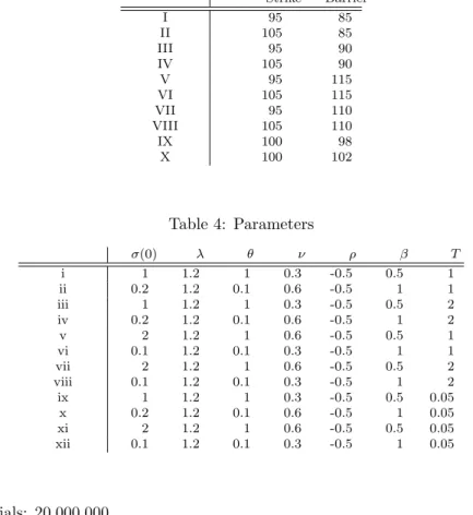
Table 1: Volatilities (η(t) =(θ+ (σ(0)−θ)e−λt)) v1 v2 v3 v4 v5 η(t) (1+3ν√T) η(t) (1+ν√T) η(t) (1 +ν √ T)η(t) (1 + 3ν√T)η(t)
Table 2: Strike Prices of Plain-Vanilla Options in Static Hedging (Strike Price = Barrier Price+γi)
γ1 γ2 γ3 γ4 γ5 T= 2 ∆ti= 0.1 0 2.5 5 7.5 10 T= 2 ∆ti= 0.4 0 5 10 15 20 T= 1 ∆ti= 0.1 0 2 4 6 8 T= 1 ∆ti= 0.2 0 3 6 9 12 T = 0.05 ∆ti= 0.01 0 0.5 1 1.5 2
Table 3: Strike and Barrier Prices of Barrier Options (I-IV, IX:out-of-the-money knock-out, V-VIII, X:in-the-money knock-out) Strike Barrier I 95 85 II 105 85 III 95 90 IV 105 90 V 95 115 VI 105 115 VII 95 110 VIII 105 110 IX 100 98 X 100 102 Table 4: Parameters σ(0) λ θ ν ρ β T i 1 1.2 1 0.3 -0.5 0.5 1 ii 0.2 1.2 0.1 0.6 -0.5 1 1 iii 1 1.2 1 0.3 -0.5 0.5 2 iv 0.2 1.2 0.1 0.6 -0.5 1 2 v 2 1.2 1 0.6 -0.5 0.5 1 vi 0.1 1.2 0.1 0.3 -0.5 1 1 vii 2 1.2 1 0.6 -0.5 0.5 2 viii 0.1 1.2 0.1 0.3 -0.5 1 2 ix 1 1.2 1 0.3 -0.5 0.5 0.05 x 0.2 1.2 0.1 0.6 -0.5 1 0.05 xi 2 1.2 1 0.6 -0.5 0.5 0.05 xii 0.1 1.2 0.1 0.3 -0.5 1 0.05 • Number of trials: 20,000,000
• Extrapolation method with
1000 and 2000 time steps for cases i, iii, vi, viii(small volatility cases) 2000 and 4000 time steps for cases ii, iv, v, vii(large volatility cases)
100 and 200 time steps for cases ix, xii(small volatility and short maturity cases) 200 and 400 time steps for cases x, xi(large volatility and short maturity cases)
Finally, the approximate values of portfolios of plain-vanilla and digital options are computed by the fifth-order asymptotic expansion scheme. Note that since the corresponding system of ordinary differential equations is solved analytically and hence a closed-form approximation formula for pricing the options is obtained, these approximate values are computed in a few seconds (about 10−1seconds for ∆t
i =T /5 and
about 1.7 seconds for ∆ti=T /20 for computing the values of the portfolios in Intel Xeon 5160 processor
at 3.00GHz.) On the other hand, if Monte Carlo simulations are applied in construction of static hedging portfolios, it is very time-consuming and hence is not useful in practice.
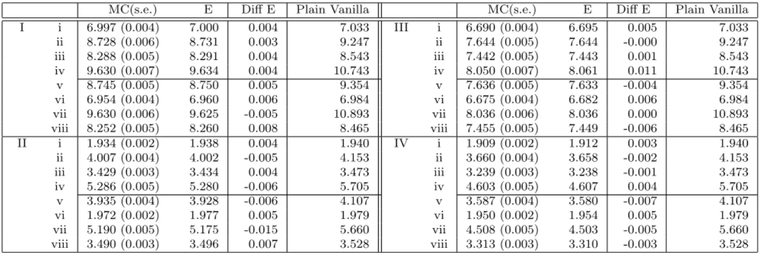
Tables 5, 6, 7 and 8 show the results. Generally, the method provides good approximations of barrier option prices. In particular, even when the number of time-steps for the static hedging is only five, our approximation method still works very well(see Table 7 and 8): Especially, Table 8 shows that use of digital options with the asymptotic expansion improves accuracies of approximations for in-the-money knock-out call option prices. This substantial reduction of time-steps makes computation speed faster, which implies an advantage of our method in practice.
Table 5: Out-of-the-money knock out: ∆ti=T /20 forT = 1,2, ∆ti= 0.01 forT = 0.05
MC(s.e.) E Diff E Plain Vanilla MC(s.e.) E Diff E Plain Vanilla
I i 6.997 (0.004) 7.000 0.004 7.033 III i 6.690 (0.004) 6.694 0.004 7.033 ii 8.728 (0.006) 8.729 0.001 9.247 ii 7.644 (0.005) 7.640 -0.004 9.247 iii 8.288 (0.005) 8.291 0.004 8.543 iii 7.442 (0.005) 7.442 0.000 8.543 iv 9.630 (0.007) 9.634 0.004 10.743 iv 8.050 (0.007) 8.061 0.011 10.743 v 8.745 (0.005) 8.748 0.003 9.354 v 7.636 (0.005) 7.629 -0.007 9.354 vi 6.954 (0.004) 6.960 0.005 6.984 vi 6.675 (0.004) 6.681 0.006 6.984 vii 9.630 (0.006) 9.625 -0.005 10.893 vii 8.036 (0.006) 8.036 0.000 10.893 viii 8.252 (0.005) 8.261 0.008 8.465 viii 7.455 (0.005) 7.448 -0.007 8.465 II i 1.934 (0.002) 1.938 0.004 1.940 IV i 1.909 (0.002) 1.908 -0.001 1.940 ii 4.007 (0.004) 4.008 0.001 4.153 ii 3.660 (0.004) 3.661 0.001 4.153 iii 3.429 (0.003) 3.435 0.005 3.473 iii 3.239 (0.003) 3.239 0.000 3.473 iv 5.286 (0.005) 5.285 -0.001 5.705 iv 4.603 (0.005) 4.610 0.007 5.705 v 3.935 (0.004) 3.937 0.003 4.107 v 3.587 (0.004) 3.584 -0.003 4.107 vi 1.972 (0.002) 1.977 0.005 1.979 vi 1.950 (0.002) 1.954 0.005 1.979 vii 5.190 (0.005) 5.181 -0.009 5.660 vii 4.508 (0.005) 4.505 -0.002 5.660 viii 3.490 (0.003) 3.496 0.007 3.528 viii 3.313 (0.003) 3.310 -0.002 3.528 IX ix 0.858 (0.001) 0.855 -0.003 0.892 x 1.321 (0.001) 1.317 -0.005 1.758 xi 1.315 (0.001) 1.313 -0.002 1.759 xii 0.859 (0.001) 0.858 -0.001 0.892
Table 6: In-the-money knock out: ∆ti=T /20 forT = 1,2, ∆ti= 0.01 forT = 0.05
MC(s.e.) E E-D E-DD Diff E Diff E-D Diff E-DD Plain Vanilla
V i 4.572 (0.003) 4.559 4.562 4.566 -0.013 -0.010 -0.006 7.033 ii 2.523 (0.002) 2.534 2.525 2.516 0.010 0.001 -0.008 9.247 iii 2.880 (0.002) 2.885 2.882 2.878 0.005 0.002 -0.001 8.543 iv 1.659 (0.002) 1.668 1.659 1.650 0.010 0.001 -0.008 10.743 v 2.721 (0.002) 2.738 2.728 2.718 0.017 0.007 -0.004 9.354 vi 4.338 (0.003) 4.335 4.337 4.338 -0.003 -0.002 -0.000 6.984 vii 1.806 (0.002) 1.817 1.807 1.797 0.011 0.001 -0.009 10.893 viii 2.669 (0.002) 2.681 2.676 2.671 0.011 0.007 0.002 8.465 VI i 0.689 (0.001) 0.684 0.686 0.687 -0.005 -0.003 -0.002 1.940 ii 0.383 (0.001) 0.395 0.391 0.386 0.012 0.007 0.003 4.153 iii 0.434 (0.001) 0.436 0.434 0.432 0.002 0.001 -0.001 3.473 iv 0.246 (0.001) 0.256 0.251 0.247 0.010 0.005 0.001 5.705 v 0.433 (0.001) 0.446 0.441 0.436 0.013 0.008 0.003 4.107 vi 0.629 (0.001) 0.629 0.629 0.630 -0.000 0.000 0.001 1.979 vii 0.281 (0.001) 0.291 0.286 0.281 0.010 0.005 0.000 5.660 viii 0.383 (0.001) 0.388 0.386 0.383 0.005 0.003 0.000 3.528 VII i 2.368 (0.002) 2.370 2.368 2.367 0.002 0.000 -0.001 7.033 ii 1.018 (0.001) 1.028 1.022 1.016 0.009 0.003 -0.003 9.247 iii 1.177 (0.001) 1.188 1.185 1.183 0.010 0.008 0.006 8.543 iv 0.618 (0.001) 0.627 0.622 0.616 0.009 0.004 -0.001 10.743 v 1.075 (0.001) 1.085 1.078 1.072 0.009 0.003 -0.004 9.354 vi 2.257 (0.002) 2.249 2.254 2.260 -0.008 -0.002 0.003 6.984 vii 0.655 (0.001) 0.662 0.657 0.651 0.008 0.002 -0.004 10.893 viii 1.117 (0.001) 1.125 1.123 1.120 0.009 0.006 0.004 8.465 VIII i 0.114 (0.000) 0.116 0.115 0.115 0.001 0.001 0.000 1.940 ii 0.046 (0.000) 0.052 0.050 0.048 0.005 0.003 0.002 4.153 iii 0.053 (0.000) 0.055 0.054 0.053 0.002 0.002 0.001 3.473 iv 0.028 (0.000) 0.032 0.030 0.028 0.004 0.002 0.000 5.705 v 0.052 (0.000) 0.057 0.055 0.053 0.005 0.003 0.001 4.107 vi 0.104 (0.000) 0.101 0.103 0.105 -0.003 -0.001 0.001 1.979 vii 0.031 (0.000) 0.035 0.033 0.031 0.004 0.002 0.000 5.660 viii 0.047 (0.000) 0.050 0.049 0.048 0.002 0.002 0.001 3.528 X ix 0.121 (0.000) 0.138 0.130 0.122 0.017 0.009 0.001 0.892 x 0.023 (0.000) 0.030 0.030 0.029 0.007 0.007 0.006 1.758 xi 0.023 (0.000) 0.025 0.024 0.024 0.002 0.002 0.001 1.759 xii 0.119 (0.000) 0.133 0.127 0.120 0.014 0.007 0.000 0.892
Table 7: Out-of-the-money knock out: ∆ti =T /5 forT = 1,2
MC(s.e.) E Diff E Plain Vanilla MC(s.e.) E Diff E Plain Vanilla
I i 6.997 (0.004) 7.000 0.004 7.033 III i 6.690 (0.004) 6.695 0.005 7.033 ii 8.728 (0.006) 8.731 0.003 9.247 ii 7.644 (0.005) 7.644 -0.000 9.247 iii 8.288 (0.005) 8.291 0.004 8.543 iii 7.442 (0.005) 7.443 0.001 8.543 iv 9.630 (0.007) 9.634 0.004 10.743 iv 8.050 (0.007) 8.061 0.011 10.743 v 8.745 (0.005) 8.750 0.005 9.354 v 7.636 (0.005) 7.633 -0.004 9.354 vi 6.954 (0.004) 6.960 0.006 6.984 vi 6.675 (0.004) 6.682 0.006 6.984 vii 9.630 (0.006) 9.625 -0.005 10.893 vii 8.036 (0.006) 8.036 0.000 10.893 viii 8.252 (0.005) 8.260 0.008 8.465 viii 7.455 (0.005) 7.449 -0.006 8.465 II i 1.934 (0.002) 1.938 0.004 1.940 IV i 1.909 (0.002) 1.912 0.003 1.940 ii 4.007 (0.004) 4.002 -0.005 4.153 ii 3.660 (0.004) 3.658 -0.002 4.153 iii 3.429 (0.003) 3.434 0.004 3.473 iii 3.239 (0.003) 3.238 -0.001 3.473 iv 5.286 (0.005) 5.280 -0.006 5.705 iv 4.603 (0.005) 4.607 0.004 5.705 v 3.935 (0.004) 3.928 -0.006 4.107 v 3.587 (0.004) 3.580 -0.007 4.107 vi 1.972 (0.002) 1.977 0.005 1.979 vi 1.950 (0.002) 1.954 0.005 1.979 vii 5.190 (0.005) 5.175 -0.015 5.660 vii 4.508 (0.005) 4.503 -0.005 5.660 viii 3.490 (0.003) 3.496 0.007 3.528 viii 3.313 (0.003) 3.310 -0.003 3.528
Table 8: In-the-money knock out: ∆ti=T /5 forT = 1,2
MC(s.e.) E E-D E-DD Diff E Diff E-D Diff E-DD Plain Vanilla
V i 4.572 (0.003) 4.634 4.602 4.571 0.062 0.030 -0.002 7.033 ii 2.523 (0.002) 2.576 2.548 2.520 0.053 0.025 -0.003 9.247 iii 2.880 (0.002) 2.970 2.926 2.883 0.091 0.047 0.003 8.543 iv 1.659 (0.002) 1.734 1.697 1.660 0.081 0.044 0.007 10.743 v 2.721 (0.002) 2.794 2.761 2.729 0.072 0.040 0.008 9.354 vi 4.338 (0.003) 4.401 4.372 4.343 0.063 0.034 0.005 6.984 vii 1.806 (0.002) 1.888 1.846 1.804 0.082 0.040 -0.002 10.893 viii 2.669 (0.002) 2.756 2.716 2.675 0.087 0.046 0.006 8.465 VI i 0.689 (0.001) 0.721 0.705 0.690 0.032 0.016 0.001 1.940 ii 0.383 (0.001) 0.419 0.405 0.391 0.035 0.021 0.007 4.153 iii 0.434 (0.001) 0.478 0.456 0.434 0.045 0.023 0.001 3.473 iv 0.246 (0.001) 0.286 0.267 0.249 0.040 0.021 0.003 5.705 v 0.433 (0.001) 0.473 0.457 0.441 0.041 0.024 0.008 4.107 vi 0.629 (0.001) 0.662 0.647 0.632 0.033 0.018 0.003 1.979 vii 0.281 (0.001) 0.325 0.304 0.283 0.044 0.023 0.002 5.660 viii 0.383 (0.001) 0.426 0.405 0.385 0.043 0.022 0.002 3.528 VII i 2.368 (0.002) 2.435 2.405 2.376 0.067 0.038 0.008 7.033 ii 1.018 (0.001) 1.064 1.045 1.027 0.046 0.027 0.008 9.247 iii 1.177 (0.001) 1.241 1.214 1.186 0.064 0.036 0.009 8.543 iv 0.618 (0.001) 0.664 0.642 0.620 0.046 0.024 0.002 10.743 v 1.075 (0.001) 1.127 1.106 1.085 0.051 0.030 0.009 9.354 vi 2.257 (0.002) 2.323 2.296 2.268 0.066 0.039 0.011 6.984 vii 0.655 (0.001) 0.702 0.678 0.654 0.048 0.024 -0.000 10.893 viii 1.117 (0.001) 1.177 1.150 1.123 0.060 0.033 0.006 8.465 VIII i 0.114 (0.000) 0.136 0.126 0.116 0.021 0.011 0.002 1.940 ii 0.046 (0.000) 0.062 0.055 0.049 0.015 0.009 0.003 4.153 iii 0.053 (0.000) 0.072 0.063 0.054 0.019 0.010 0.001 3.473 iv 0.028 (0.000) 0.043 0.035 0.028 0.015 0.007 0.000 5.705 v 0.052 (0.000) 0.068 0.061 0.054 0.016 0.009 0.002 4.107 vi 0.104 (0.000) 0.124 0.115 0.106 0.020 0.011 0.002 1.979 vii 0.031 (0.000) 0.047 0.039 0.031 0.016 0.008 0.000 5.660 viii 0.047 (0.000) 0.066 0.057 0.048 0.019 0.010 0.001 3.528
5
Pricing Average Options
This section applies the high-order expansion scheme described in Section 3 to pricing average options. In particular, we describe the method using numerical examples under theλ-SABR and SABR models.
5.1
Average Options under
λ
-SABR and SABR Models
We consider the average European call and put options under theλ-SABR model (17) with interest rate=0% for simplicity. In particular, whenλ= 0 the model becomes the SABR model. Further, we define
S(Aϵ)(t) =
∫ t
0
S(ϵ)(u)du.
Then, the average European call option price with strikeKand maturity T can be written as
CA(ϵ)(K, T) =E [ max { 1 TS (ϵ) A (T)−K,0 }] .
Thus, if we consider the following three-dimensional diffusion process, we can easily see that it is a special case of (1) and the general method explained in Section 3 can be applied:
dSA(ϵ)(t) = S(ϵ)(t)dt,
dS(ϵ)(t) = ϵσ(ϵ)(t)(S(ϵ)(t))βdWt1,
dσ(ϵ)(t) = λ(θ−σ(ϵ)(t))dt+ϵν1σ(ϵ)(t)dWt1+ϵν2σ(ϵ)(t)dWt2 (18)
withSA(ϵ)(0) = 0,S(ϵ)(0) =S
0 andσ(ϵ)(0) =σ.
The corresponding differential equations up to the second order are given by
d dtη S 1,1(t;ξ) = (iξ)(S (0) t )βσ (0) t Vˆ(t), d dtη σ 1,1(t;ξ) = (iξ)ν1σ (0) t Vˆ(t)−λη σ 1,1(t;ξ), d dtη SA 2,1(t;ξ) = η S 2,1(t;ξ), d dtη S 2,1(t;ξ) = 2(iξ)β(S (0) t ) β−1σ(0) t Vˆ(t)η S 1,1(t;ξ) + 2(iξ)(S (0) t ) βVˆ(t)ησ 1,1(t;ξ), whereSt(0)=S0,σ (0) t =e−λt(σ−θ) +θand ˆ V(t) = (T−t)(S(0)t )βσ(0)t .
Then, the asymptotic expansion of the density function of ˜G(ϵ)= SAT(ϵ)−SAT(0)
ϵ can be obtained as fG˜(ϵ)(x)≈fg1T(x) +ϵC˜13H3(x; ˜ΣT)fg1T(x) +· · · (19) where fg1T(x) = 1 √ 2πΣ˜T exp ( − x2 2 ˜ΣT ) with ˜ ΣT = ∫ T 0 ˆ V(t)2dt and ˜ C13 = 1 ˜ Σ3 T ∫ T 0 ∫ t1 0 ∫ t2 0 β(S(0)t 2 ) β−1σ(0) t2 ˆ V(t2)(S (0) t3 ) βσ(0) t3 ˆ V(t3)dt3dt2dt1 + 1 ˜ Σ3 T ∫ T 0 ∫ t1 0 ∫ t2 0 e−λ(t2−t3)(S(0) t2 ) βVˆ(t 2)ν1σ (0) t3 ˆ V(t3)dt3dt2dt1.
As in the plain vanilla case described in Section 3.1, integrals appeared in the coefficients of the expansion can be analytically evaluated, but the expressions are lengthy and hence omitted. Moreover, by a sim-ilar calculation to Section 3.2, we have the following closed-form approximation formula for the average European call option up toϵ2:
CA(ϵ)(K, T) = ϵP(0, T) ( ˜ ΣT T fg1T(y) + y TN ( y √ ˜ ΣT )) −ϵ2P(0, T) ˜ C13Σ˜2Ty T fg1T(y) +o(ϵ 2), (20) wherey= T S0−T K
ϵ andP(0, T) denotes the price at time 0 of a zero coupon bond with maturityT .
5.2
Numerical Examples
This subsection provides some numerical examples of our asymptotic expansion method for pricing average options under the λ-SABR and SABR models to see the effectiveness of the higher order asymptotic expansions. Further, as a special case of the SABR model, we apply our method to the constant volatility case (Black-Scholes model) and compare approximation accuracies of our method with those of other approximation methods.
5.2.1 Constant Volatility Case
First, we apply our method to the constant volatility case (the Black-Scholes model) which is obtained by setting λ=νi = 0(i = 1,2) and β = 1 in (18). Then, the asymptotic expansion of the density function
(19) can be simplified as fGBS˜(ϵ)(x)≈f BS g1T(x) +ϵ ˜ C13BSH3(x; ˜ΣBST )fgBS1T(x) +· · ·, where fg1BST(x) =√ 1 2πΣ˜BS T exp ( − x2 2 ˜ΣBS T ) with ˜ ΣBST = ∫ T 0 (T−t)2σ2S02dt=1 3σ 2S2 0T 3, ˜ C13BS = 1 ( ˜ΣBST )3 ∫ T 0 ∫ t1 0 ∫ t2 0 (T−t2)(T−t3)σ4S03dt3dt2dt1= 1 5σ 2S 0T2. (21)
A closed-form approximation formula to the average European call option under the Black-Scholes model can be obtained by replacing ˜ΣT and ˜C13by ˜ΣBST and ˜C
BS
13 respectively in (20).
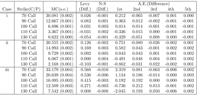
In the Black-Scholes case, unlike the stochastic volatility cases, there are several approximation methods for pricing an average option. Here we compare approximation accuracies of our asymptotic expansion method with those of these existing methods.
We consider the average European call option under the Black-Scholes model. We calculate approx-imated prices of average options by the asymptotic expansion method up to the fifth order and we also calculate approximated prices by the moment matching method given by Levy[22] and by the lower bound for average options given by Nielsen and Sandmann[27].
In the numerical examples,ϵis set to be one and other parameters are given in Table 9.
Benchmark values are computed by Monte Carlo simulations. We use the second order scheme given by Ninomiya-Victoir[28] as a discretization scheme with 128 time steps for case i, and with 256 time steps for case ii and iii respectively. We adopt Mersenne-twister as a random number generating engine, and generate 5×10⁷ paths with antithetic sampling in each simulation. We calculate the lower bound given by Nielsen and Sandmann with 1024 time steps.
Table 9: Parameters for the Black-Scholes Models
Case S(0) σ T
i 100 0.3 1
ii 100 0.3 2
iii 100 0.5 2
Table 10: Approximation errors for average call options under Black-Scholes model.
Levy N-S A.E.(Difference)
Case Strike(C/P) MC(s.e.) (Diff.) (Diff.) 1st 2nd 3rd 4th 5th i 70 Call 30.081 (0.002) 0.026 -0.001 0.212 -0.065 -0.007 0.001 0.000 90 Call 12.667 (0.001) 0.082 0.001 0.363 0.012 -0.002 -0.001 -0.001 100 Call 6.896 (0.001) 0.031 0.003 0.014 0.014 -0.001 -0.001 -0.001 110 Call 3.367 (0.001) -0.031 0.002 -0.336 0.015 0.000 -0.001 -0.001 130 Call 0.622 (0.000) -0.054 -0.001 -0.329 -0.051 0.008 0.000 -0.001 ii 70 Call 30.555 (0.002) 0.126 -0.002 0.751 -0.080 -0.026 -0.002 0.001 90 Call 14.993 (0.002) 0.169 0.003 0.582 0.043 -0.001 0.002 0.002 100 Call 9.729 (0.002) 0.092 0.005 0.043 0.043 0.001 0.001 0.002 110 Call 6.067 (0.001) 0.000 0.004 -0.491 0.048 0.004 0.001 0.002 130 Call 2.168 (0.001) -0.103 -0.001 -0.862 -0.031 0.022 -0.002 0.001 iii 70 Call 33.179 (0.004) 0.568 -0.016 2.319 0.081 -0.063 -0.006 0.002 90 Call 20.639 (0.004) 0.536 -0.006 1.134 0.186 -0.014 0.000 0.003 100 Call 16.095 (0.003) 0.415 -0.003 0.192 0.192 0.000 0.000 0.003 110 Call 12.509 (0.003) 0.271 -0.003 -0.736 0.212 0.013 -0.001 0.002 130 Call 7.542 (0.002) 0.008 -0.008 -2.045 0.193 0.050 -0.006 0.002
Benchmark prices by Monte Carlo simulations and their standard errors are given in Table 10. Also, approximation errors of the moment matching method(Levy), the lower bound given by Nielsen and Sandmann(N-S) and of our asymptotic expansions are reported in Table 10.
From the results above, asymptotic expansions almost always improve the accuracy of the approximation as the order of expansion increases and the forth or fifth order asymptotic expansion have smaller or equal approximation errors to those of other methods. Further, as seen in the next subsection, our method can be extended in the same framework to the stochastic volatility case where these other methods cannot be applied.
5.2.2 Stochastic Volatility Case
Next, we consider the stochastic volatility case such asλ-SABR/SABR model described in (18).
In the following numerical example, approximated prices by the asymptotic expansion method are calculated up to the fourth order for the λ-SABR model and up to the fifth order for the SABR model respectively. Note that all the solutions to differential equations are obtained analytically. Benchmark values are computed by Monte Carlo simulations. ϵis set to be one and other parameters used in the test are given in Table 11 for theλ-SABR case (i, ii and iii) and the SABR case (iv, v and vi).
In Monte Carlo simulations for benchmark values, we use Euler-Maruyama scheme as a discretization scheme with extrapolation method with 256 and 512 time steps for case i, ii, iv, v and with 512 and 1024 time steps for case iii and vi respectively. In each simulation, we generate 5×10⁷ paths with antithetic sampling.
Results are in Table 12 for the λ-SABR case and in Table 13 for the SABR case respectively. Since the solution to the system of ordinary differential equations is solved analytically, computing time for the asymptotic expansions is less than 10−3 seconds which is much shorter than that for the Monte Carlo
Table 11: Parameters for theλ-SABR models Case S(0) β σ(0) λ θ ν ρ T i 100 1.0 0.3 1.0 0.3 0.3 -0.5 1 ii 100 1.0 0.3 1.0 0.3 0.6 -0.5 1 iii 100 1.0 0.3 1.0 0.3 0.3 -0.5 2 iv 100 1.0 0.5 0 - 0.5 -0.5 1 v 100 0.5 3.0 0 - 0.3 -0.5 1 vi 100 1.0 0.5 0 - 0.5 -0.5 2 simulations.
Table 12: Asymptotic expansions for average options under theλ-SABR model up to the fourth order
A.E.(Difference) Case Strike(C/P) MC 1st 2nd 3rd 4th i 50 Put 0.000 (0.000) 0.009 -0.010 0.003 -0.001 80 Put 0.804 (0.000) 0.261 0.011 0.004 0.003 100 Call 6.873 (0.001) 0.036 0.036 0.005 0.005 120 Call 1.306 (0.000) -0.240 0.010 0.004 0.005 150 Call 0.046 (0.000) -0.036 -0.017 -0.004 0.000 ii 50 Put 0.005 (0.000) 0.005 -0.001 0.007 -0.001 80 Put 0.988 (0.000) 0.078 0.002 0.030 0.007 100 Call 6.886 (0.001) 0.024 0.024 0.007 0.007 120 Call 1.183 (0.000) -0.117 -0.042 -0.014 0.009 150 Call 0.035 (0.000) -0.025 -0.020 -0.012 -0.004 iii 50 Put 0.024 (0.000) 0.162 -0.076 -0.001 0.001 80 Put 2.251 (0.001) 0.609 0.060 0.004 0.003 100 Call 9.685 (0.002) 0.088 0.088 0.001 0.001 120 Call 3.348 (0.001) -0.488 0.061 0.005 0.006 150 Call 0.495 (0.000) -0.309 -0.071 0.004 0.002
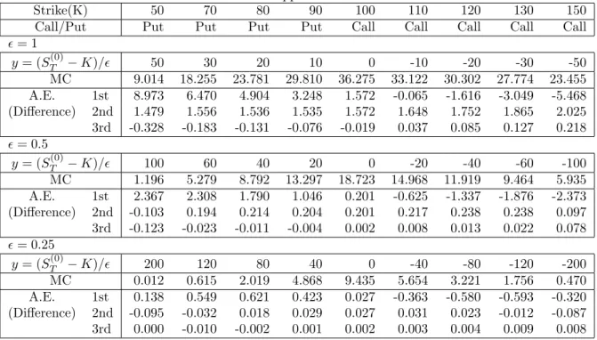
From the results above, in each case the higher order asymptotic expansion almost always improves the accuracy of approximation by the lower expansions. In particular, the higher order asymptotic expansions effectively approximate the prices in long-term cases or high-volatility of volatility (ν) cases in which the lower order asymptotic expansions can not approximate the prices well.
Finally, we remark that in the asymptotic expansion method the approximate density functions are expressed as a product of polynomials and the Gaussian density function: Because these polynomial-based approximation functions have wavy forms, higher order approximation sometimes provides worse approximation to the density at particular values (and to the option prices at particular strikes) than lower ones as seen in Table 12 and 13. However, on average absolute differences decrease as higher order correction terms are included.
Table 13: Asymptotic expansions for average options under the SABR model up to the fifth order A.E.(Difference)
Case Strike(C/P) MC(s.e.) 1st 2nd 3rd 4th 5th
iv 50 Put 0.137 (0.000) 0.351 -0.034 0.027 -0.014 -0.012 80 Put 3.496 (0.001) 0.679 0.136 0.038 0.014 0.002 100 Call 11.359 (0.002) 0.158 0.158 0.020 0.020 0.007 120 Call 4.623 (0.001) -0.448 0.096 -0.001 0.023 0.011 150 Call 0.964 (0.001) -0.476 -0.091 -0.029 0.013 0.015 v 50 Put 0.008 (0.000) 0.002 0.002 0.003 0.001 0.000 80 Put 1.054 (0.000) 0.012 0.012 0.013 0.005 0.004 100 Call 6.897 (0.001) 0.013 0.013 0.007 0.007 0.006 120 Call 1.070 (0.000) -0.004 -0.004 -0.003 0.005 0.003 150 Call 0.012 (0.000) -0.002 -0.002 -0.002 0.000 -0.000 vi 50 Put 0.854 (0.000) 1.324 0.170 0.132 -0.020 -0.067 80 Put 6.883 (0.001) 1.321 0.454 0.120 0.049 -0.020 100 Call 15.824 (0.003) 0.463 0.463 0.073 0.073 0.002 120 Call 8.713 (0.002) -0.509 0.357 0.023 0.093 0.024 150 Call 3.339 (0.001) -1.162 -0.008 -0.046 0.106 0.060
6
Conclusions
This paper proposed a new approximation method for pricing barrier and average options under stochastic volatility environment by applying an asymptotic expansion approach which enabled us to calculate high-order expansions easily.
For pricing barrier options, it combined an asymptotic expansion scheme with a static hedging method by Fink [9]. Applying an asymptotic expansion method to approximation of the values for the hedging option portfolio, it obtained a closed-from approximation formula for barrier options which can be easily calculated. Through the numerical examples under the λ-SABR model, it was shown that using the fifth-order asymptotic expansion scheme, our method had sufficient accuracy of the approximation. Also, numerical examples showed that using digital options had advantages in both approximation accuracy and computational speed for the valuation of in-the-money knock out options.
For average options, to our knowledge, this paper is the first one that implements the fourth and fifth order asymptotic expansion under theλ-SABR and SABR models and examines its numerical accuracy. Numerical experiments showed that the higher order expansions generally approximated the prices of the average options in longer-term or/and higher-volatility of volatility cases better than the lower order expansions.
Finally, the proposed method is general enough to be applied to other multi-dimensional diffusion models such as local-stochastic-volatility models [29] including the quadratic Heston model [1]. Thus, comparison of various models for pricing barrier and average options can be implemented based on the calibration to liquid plain-vanilla options in actual markets, which is one of our main research topics in the next step.