Work Models For Mobile Advertising

LIBRARY OF THE

MASSACHUSETTS INSTITUTE OF

TECHNOLOGY

IP'

i

WORKING

PAPER

ALFRED

P.

SLOAN SCHOOL

OF

MANAGEMENT

ADVERTISING BUDGETING AND GEOGRAPHIC ALLOCATION Glen L. Urban 4A1-70 January 1970

MASSACHUSETTS

INSTITUTE OF

TECHNOLOGY

50

MEMORIAL

DRIVE

,IDGE,

MASSACHUSETTS

02139

MA65:lfPT,T£CH.

m

3

197a

eiWIY LIBRARY

ADVERTISING BUDGETING AND GEOGRAPHIC ALLOCATION Glen L. Urban

4A1-70

970

!/l. I. .. k-1Lji\Mr\l£S

1^0^^

I I

ADVERTISING BUDGETING AND GEOGRAPHIC ALLOCATION by Glen L. Urban

ABSTRACT

This paper presents a model to aid in determining a total advertising budget and allocating it to a national media and local expenditure in each

of a number of heterogeneous geographic areas. The model includes con-sideration of area differences in advertising response, media efficiency and impact, distribution levels in areas, and carryover effects. A

"good" and hopefully "best" budget and allocation is found by a multi-stage, on-line heuristic. An application of fhis model indicates that

it has the potential to improve decisions and lead to implementation.

INTRODUCTION

When an organization views its market as a group of heterogeneous geographic segments, the problem of determining how much to spend on advertising becomes a problem of simultaneously budgeting and allocating

funds. The solution to this problem is a local advertising strategy. The

purpose of this paper is to develop and demonstrate a model to aid in

determining local marketing strategy.

The problem of overall budgeting for advertising has received much attention, and some game theoretical aspects of allocation have been

dis-2

cussed. But there is evidence to indicate that this theory is not being

3

utilized in allocating promotional expenditures. The first criteria for this author's model is that it lead to application. The second criteria

The author greatfully acknowledges that the programming for the

system was done by Jay Wurts.

2

See [4], pp. 115-137 for discussion of existing theory.

^See [3].

2.

is that the model include the major theoretical and behavioral phenomena important in this problem. These include differences in area potential, growth ratess advertising responsiveness, media costs and efficiencies, profit margins, competition, and carryover. The third criteria is that the model be a starting point for an evolutionary system that would lead from the initial aggregate one variable model to a more detailed multi-variate model. The final criterion is that the model structure lead to data based parameter estimates

»

In defining the specific problem to be attacked by the model a clear distinction must be drawn between the budgeting decision and other advertising decisions. First, it is assumed that the appeal has been selected and that a reference state defined by a starting point forecast

of sales for a starting point budget have been determined. The problem

to be studied is how to find the best total budget and geographic allocation

of that budget given the appeal and reference state conditions. After these budget decisions have been made, a media schedule would be developed and executed. A media model would not solve the budgeting and allocation problem since most media models do not link their schedules to the sales

and profit criteria of budgeting. A model such as MEDIAC which makes this

linkage also would be unsuitable since _in a market with say 30 local

segments-the number of media options would be much beyond the capacity of the media model. If a simplification of one media per area were made, the media model might be used to examine allocations, but the media model overhead in

con-sidering exposure and duplication would make this procedure inefficient.

BEMERALBCXJKBINDINOCO.

^jV2 C5I

• -7 Dr.)

QUALITYCONTROL MARK

The interaction between media models and the budgeting model developed in this paper would be iterative. The budgeting model would specify a dollar allocation for each area assuming an average set of media performance

characteristics. Then the media model would select a best schedule subject

to this budget constraint. If the schedule had better average characteristics than the budgeting model had assumed, the budgeting model would be re-run with the new characteristics and the iteraction would continue until the

budgeting assumptions and media schedule results agreed.

This paper will develop the model for local advertising response, specify the models input needs, discuss the heuristic procedure used to

find the best strategy, outline the model's limitations and extensions, and present a real application of the model.

LOCAL STRATEGY MODEL Local Advertising Response;

The first step in structuring local advertising response is to

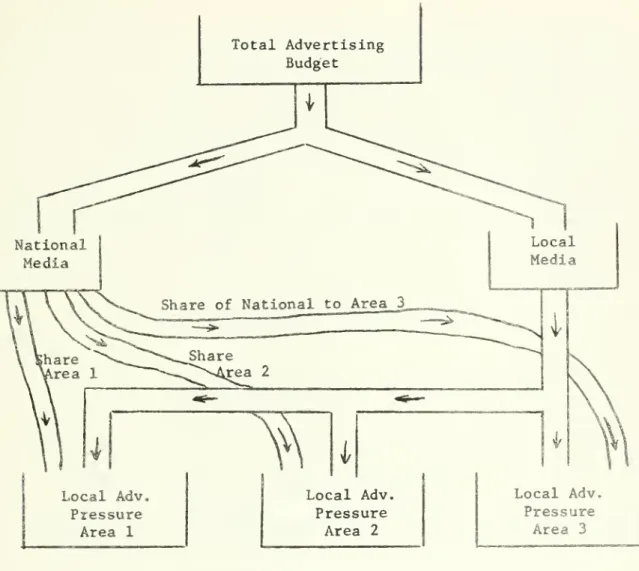
define an operational measure of the advertising pressure that exists in an area. Consider the basic flow of advertising expenditure. Part

of the total budget goes to national media with some share of this falling

on a local area and part directly to a local area. See Figure One. The advertising that is seen in a local area is either from national or local media. The concept of weighted advertising is used to define a common measure for advertising pressure on an area. Weighted advertising is

defined as the share of national expenditure in an area plus the local expenditure weighted for media exposures, impact, and efficiency. The

Total Advertising Budget Local Adv Pressure Area 1 Local Adv. Pressure Area 2 Local Adv. Pressure Area 3

weighting is based on a ratio of the rated exposure value per dollar in the local area to the rated exposure value per dollar in national media. The rated exposure value is the sum of the exposures in each media multiplied

by a media rating which reflects its impact given someone is exposed. The rated exposure value per dollar is the rated value divided by the advertising expenditure required to obtain It. The weighted advertising in a local area is;

(1) WTADVL = ADVNAT • SHRLOC • EFFNAT + ADVLOC

a,r,t t a.r.t t a,r,t

•

^^^a.r.t

. RIMPCT

REVND, '

t

= _{weighted advertising} in local area a of region r in

time period t

= _{dollar expenditure on national} media in period t

= share of national media expenditure that falls in

area a of region r in period t

= effectiveness of national media at time t^ (Set to

1.0 initially).

= local advertising dollar expenditure in area a in

region r in period t

= rated exposure value locally per dollar in local area a of region r in period t

= rated exposure value nationally per dollar in period t

= impact of local media relative to national media in

area a of region r in period t. (Set initially to 1.0)

EFFNAT is an index which can be used to change the effectiveness of national media expenditure and RIMPCT is an index which can be used to change the

impact of local expenditure relative to national. For example, these indexes may be used if new _{media opportunities appear.} ^'^^ regional subscripts are

defined so that allocations can be conducted on only specific regions if this is desired.

VIADVL a,

Having defined a measure of advertising pressure in a local area, the

next task, is to specify how it affects sales. A general function is used

to relate weighted advertising and sales. Initially, sales are specified by:

(2) TSALEL = RSALEL • ADVRSP (WTADVL _^ / WTADVLR )

^ ' _{a.r.t a,r,t a,r a,r,t} a,r,t

TSALEL = temporary forecast of sales in local area a of

region r in period t

RSALELl = reference sales in local area a of region r in period t

''^'

if reference advertising plan is carried out

ADVRSP = function describing proportionate changes in sales

''^

from reference (RSALEL, _ ,.) for a change in weighted

a»*• >^

advertising (WTADVL, _. ^) relative to the weighted

a,t»L

advertising implied by the reference planfOTADVLR )

The function (ADVRSP) will generally experience diminishing returns, but

must be determined for each area. Given this curve, the change in sales

from reference can be predicted for changes of advertising from the reference. The forecasted sales level (TSALEL) is next adjusted for distribution effects and carryover effects.

Although the model is primarily an advertising model, the distribution differences between areas are included. This is a first step in the evolutionary development that will eventually lead to a full marketing mix local strategy model. With distribution included, changes in distribution can be reflected

in the best advertising strategy. Distribution is included in the model by adjusting sales to full distribution sales and then multiplying by the per-cent of the market covered by an alternate distribution plan. The adjusted sales level (ASALEL) is:

(3) ASALEL ^ = (TSALEL ^ / AVAIL (RDISTL )) • AVAIL (DISTL

'

^ ' _{a,r,t a.r,t a,r a,r,t a,r a,r,t}

AVAIL = percent of market covered at a given distribution level a,r

(DISTL

A

in area a of region r in period t

a, r,t

RDISTLg = reference distribution level in area a _of region r

* ' _{in period t}

DISTL . = distribution level in area a of region r in period t

• a sr5

1

The distribution level is defined as the percent of outlets that carry

the product and is functionally related to the percentage coverage by AVAIL,

The phenomenon of carryover effects is included in the model by specifying how much of the change in sales from reference in one period is retained in the next period. The model considers the carryover in terms of

changes since the starting point plan implies the carryover for the reference allocation. The change in sales in area a in region r and period t-1 is: DSALEL , = SALEL _{^ ,} - RSALEL ^ ,

a,r,t-l a,r,t-l a,r,t-l

SALEL = sales in area a in region r in period t-1. (See Eq. 5),

a^r^t-l

RSALEL , = reference sales in local area a in region r in period t-1 ' ' _if reference advertising plan _is carried out.

The amount of this sales change that is retained from the last period is:

(4) RETSLL^ , = DSALEL^ , • RETRT^

a,r,t-l a,r,t-l a,r

RETSLL _^ = retained sales in area a of region r from period t-1

RETRT = retention rate for area a of region r

a,r

The retention rate reflects the brand loyalty of buyers and the competitive conditions in the local area. The retained sales will effect the sales of the next period. The model reduces this period's sales by the proportion of

8.

(5) SALEL ^ = ASALEL ^ • _(1+RETSLL

, / RSALEL ,)

a,r,t a,r,t a,r,t-l a,r,t-l

This proportionate change assumes that the original seasonal pattern of

reference sales is maintained since it presumes the retained sales follow

the seasonal pattern.

Given the above relationships the model will determine the sales

in an area given an advertising and distribution strategy. The profit in a local area Is:

(6) PROFL ^ = SALEL ^ • PMARGN _^ - ADVLOC, - SFC

a,r,t a,r,t a.r.t a,r,t a,r,t

PMARGN = contribution margin in area a of region r and time t I)r,t

SFC _^ = semi-fixed costs in area a of region r in period t a,r,L

The national profit is the total of the profit in each area less national media expenditure (ADVNAT) and the total profit over a planning period is obtained by summing national profit.

The model will determine sales and profits for alternate advertising strategies when given a starting point sales-advertising plan and the

response measures. Input to Model;

The parameters required by the model are given in Figure Two, along with the source of the input. This data is stored in the data bank and processed by statistics to the determine model input. It is beyond the

scope of this paper to discuss the statistical issues of estimation, but it is clear that careful experimental design and statistical regression

Input Name Source of Data I Reference Plans Sales RSALEL (2) Planned advertising ADVNAT (1) ADVLOC (1) Planned distribution RDISTL ₍₃₎ Internal forecasting mechanism II Exposure Data REVND (1) REVLD (1) SHRLOC (1) Advertising agency

III Response Measures Retention rates RETRT (4) Advertising response ADVRSP (2) Distribution response AVAIL (3) Statistical analysis of past data or experimentation IV Profit PMARGN (6) SFC (6) Accounting records Equation numbers

10.

are required. Even after the most careful statistics, subjective juHg-ments may also be required in specifying the best set of input.

Heuristic Solution Procedure:

Since the proposed model is a multiperiod model with carryover effects and has a complex response mechanism (ioe= dollars to weighted advertising to sales) the algorithmic procedures of linear and non-linear programming are not applicable to the problem of finding the best budget and allocation. To attempt to find the "best" budget and allocation, a multi-stage interactive heuristic is used. The heuristic solution

pro-cedure exists at three levels: "allocate", "split" and "search". At

each level the man interacts with the procedure so that the knowledge of the manager and the power of the search rule can be combined to efficiently find the best strategy,

"Allocate" takes the total budget and national advertising as given and allocates the total local expenditure to each area in an attempt to

maximize the total profit over the planning period. The steps of "allocate" are

1. Calculate the marginal rewards to local advertising (ADVLOC in

Eq. 1) in each area. That is, additional profit generated by

changing local advertising expenditure. This is generated by removing a percent of advertising (DELALL) in an area in each time period, calculating the change in total profits over the

planning period in that area, and dividing by the total value

of the advertising taken out. The amount of advertising change is summed over the planning period and is called TMOVED.

See application section of this paper for an example of the estimation procedure.

11.

2. In each area check to see if moving on "S" shaped response curve

by evaluating marginal reward for 2 x DELALL reduction in local advertising. If marginal for 2 x DELALL is less than marginal

for 1 X DELALL, remove area from consideration unless management

is willing to abandon local area. If marginal for 2 x DELALL is greater than 1 x DELALL, add area to list for consideration.

3. Find the areas with the largest and smallest marginals on list of areas to be considered. Define TMOVED = _TMOVED for low area

La

(L) and TMOVEDj^ = TMOVED for high area (H) ,

^' _{If the high marginal minus the low marginal} as a percent of the

absolute value of the high marginal is greater than the tolerance

(TOLALL) , go to 5. If not, stop.

5. Is new high area the same as the low area at last iteration, and is the new low area the same as the high area at the last iteration? If yes, stop. If no, go to 6.

6. If TMOVED^ < TMOVED^, MOVE = TMOVED and go to 7. If TMOVED >

TMOVED„, MOVE = _TMOVED^ and go to 7.

n H

7. Change advertising levels by removing MOVE from low area (L) and adding MOVE to high area (H). Revise levels in each period in

proportion to MOVE relative to total local advertising in area over planning period.

8. Calculate new marginals based on DELALL for areas where local advertising has been changed. Go to 2.

12.

The allocation heuristic is controlled by the amount of advertising moved

(DELALL) and the tolerance (TOLALL) . A good procedure is to start with a

large DELALL (e.g. 25%) and TCLALL (e.g. 25%) and then after finding a

solution repeat with a lower DELALL and TOlALL. Step two assures that if

cur-rent advertising is on an upward concave section of an "S" shaped advertising response curve, the heuristic will not lead to removing all advertising

from the area unless this is acceptable. An "S" curve may reflect short run considerations in the area and not the long run possibilities for

changes in the area that would warrent its maintenance. For example, a

low distribution level might be increased in the future. Step 5 prevents

a cycling in the heuristic. Step 6 assures that the amount moveH from one area does not become an overbearing amount. This is important if budgets vary

widely between areas. Step 7 changes the advertising levels proportionately so that the seasonal pattern of expenditure in the area will be maintained. The heuristic continues until a best allocation of local expenditure is

found within the specified tolerance.

"Split" takes the total budget as given and determines how much is

split to national media and how much to local media (see Figure 1). Split begins moving expenditures from local to national. If it finds this

successful, it continues until insufficient improvement occurs. If split finds the initial movement unprofitable, it moves expenditure from national to local and continues in this direction if there is sufficient improvement. The steps of "split" are:

13.

1. Move a percent of local expenditure (PSPLIT) to national, use "allocate" to find best local allocation, and determine the change

in total profit over the planning period.

2. If the change is more than a minimum percent increase (TOLSPT)

,

go to 1. If not, go to 3 unless have moved some amount from

local at the last iteration. In this case stop.

3. Move a percent of national expenditure (PSPLIT) to local, use "allocate" to find best local allocation, and determine the

change in total profit over the planning period.

A. If change in profit is greater than minimum percent increase (TOLSPT), go to 3; otherwise stop.

Split is controlled by the percent moved (PSPLIT) and the tolerance (TOLSPT).

Split increments from the best pattern of allocation. This pattern recall minimizes the computation in subsequent utilizations of the allocate heuristic.

"Search" evaluates a number (NSTEP) of total budget alternatives. The steps are:

1. Sequentially examine alternatives in increments (DELBG) above reference. Use "split" for each alternative.

2. Return to reference plan and evaluate specified alternatives sequentially in increments (DELBG) below reference. Use "split" for each alternative.

3. Record best alternative.

Search begins at reference and examines the specified alternatives sequentially from the reference. After each alternative it records the best split and

14.

allocation patterns so that the evaluation of the next alternative will

begin from the previous best pattern and therefore will require less

computation to find the new best plan.

The multi-stage heuristic is implemented in an on-line interactive computer program. In this way a manager or researcher can interact with

the power of the heuristic to find a good solution. The man is important since he has experience and pattern recognition capabilities that can be

useful in effeciently finding solutions. He can specify or change the

starting points, examine desired total budgets and iteratively converge on the best solution by changing the search increments (DELBG, PSPLIT, DELALL) and tolerances (TOLSPT, TOLALL). The multi-stage feature is useful

if a budget is prespecified and only the split between national and local media is to be considered at a given time. Another example is the use of the system by a regional manager who only wants to allocate a local budget for his region. The on-line feature of the system also allows parameters

to be changed at any stage so sensitivity testing can be conducted on

parameters that are in doubt.

The output of the heuristic when applied to the model is a best total budget, split between national and local expenditure, and budget allocation

for each geographic area. By changing distribution levels, the interaction between advertising strategy and distribution can be assessed. Similarily,

the on-line change mechanism fosters a sensitivity analysis. The interactive program and model structure are designed to promote application by involving

15.

managers and data in a reasonable description of the market structure so as to improve the determination of local strategies. The model can also function as a control mechanism when applied on a continuing basis. With continuing experimentation the model could be imbedded in an adaptive planning system.

Limitations and Extensions of the Model:

This model encompasses the major factors and phenomena in the

budgeting problem, but the consideration of some of them is quite simple and could be extended in future work. For example, the competitive effects

are included indirectly in each area's retention rate (see Eq. 4) along with brand loyalty. This assumes competitors will behave as they have in

the past despite our advertising changes. The future evolutionary develop-ment of the model could separate the competitive effect. This could be

accomplished by making advertising response (ADVRSP, Eq. 2) a function of our expenditure relative to competition or, more eloquently, by creating

a ratio of our advertising to the sum of all firms' advertising, each raised

Q

to a sensitivity exponent. With an explicit competitive formulation, payoffs could be found for various competitive strategies^and Bayesian decision or

game theory procedures could be utilized. Other extensions to the model could be made to include other variables such as price and promotion through additional response functions and to include overlaps between areas.

''see [1]. g

16.

The heuristic could be extended to explicitly include the sequence

of advertising levels. In its current form, the heuristic takes the

sequence as given and increments it. Although the sequence could be changed on-line and the heuristic re-run, it would be useful to

consider both the level and pattern of expenditure. Although simple, it is hoped that this model is a good base for future developments that

would produce a multi-variate local strategy model with a dynamic heuristic and statistical support system.

APPLICATION Input and Parameter Estimation;

This budgeting and allocation model has been applied to a frequently purchased consumer product marketed by a medium sized firm. The data base available was; 1. sales data for 60 months, 2. advertising contract buys

for 60 months, 3. percent of outlets carrying product in each year, 4, audiences

of media by area by year, and 5. contribution margin by area by year.

Monthly time periods were used for the input analysis. The areas used were the 20 largest market areas and the residuals of non-top 20 areas by region. The data on advertising was combined by calculating the weighted advertising (see Eq. 1) and used as a measure of advertising pressure in

each area in the statistical analysis to determine advertising response.

In all the statistical analysis, the data for the last 12 months was not examined. It was "saved" so that the model could be compared to

the actual results.

Exploratory plots and regressions of the monthly sales, advertising and distribution data were conducted in an effort to diagnose problems and

17.

overall relationships in the data. The plots indicated (1) a strong

seasonal pattern with highest sales in the summer, (2) advertising did not

follow the seasonal pattern

—

largest advertising generally occurred in

the fall, (3) a growth trend in most areas, (4) considerable fluctuation

in sales from trend and seasonal patterns, and (5) no specific one or two

month lag in sales and advertising (that is, advertising increases in

period t did not seem to always produce a sales increase in t+1)

.

Exploratory regressions were run in each area on a step-wise basis. Distribution did not enter the equations due to the yearly nature of the

distribution and its small variation. Log-linear response forms did not

improve the exploratory power or significance of the regressions over the

range of data, so linear equations were adopted as the standard form. These linear equations provide an estimate of the marginal response to advertising

in the data range. The exploratory analysis indicated that a distributed

lagged term (sales ^) was significant and large (70% of the areas had a

value greater than .8). Although a specific lag was not present, an

exponential decay of sales was present. The values of advertising response

in these exploratory equations were generally negative. This was counter intuitive, but was due to the contra-cyclical nature of advertising. Low advertising with high sales (summer) and high advertising with lower sales

(fall). Tliis indicated future regressions would have to carefully separate

seasonal sales and advertising effects.

The formal time series regression analysis used the following equation:

18.

Sales^ = b_ + b-jD^ + b„D- + b-advertising^ + b.sales^ .

t

011223

°t4

t-1

r

1 ir C. ot 1 in summer otherwise „ , _ in winter )therwise

D^ and D- are dummy variables that are specified in an attempt to

deseasonallze the data. The results of these regressions are shown in

Table 1. All the F statistics were significant at 10% level. The retention rates are generally significant and positive, but the advertising coefficients

are low when positive and sometimes significantly negative. The retention

rates were acceptable, but it was suspected that advertising and sales effects wert

confounded. In an attempt to separate the seasonal effects, a prior seasonal model was developed for each area. This model de-seasonalized the data on the basis of an index derived from areas where advertising did not change over the seasonal pattern. Unfortunately, this effort was not successful. Finally, a twelve month change model was run for each area. In this model

the change in sales in month "t" minus sales twelve months earlier was regressed against the change in advertising between those periods. This again was unsuccessful in separating the effects of the seasonal sales and advertising response.

Although the advertising response values were counter intuitive

due to the confounding of the seasonal and advertising response, the

regression model was good on a predictive test against the saved 12 months

19. area 1 2 3 4 5 6 8 9 10 11 12 -.8, -.A, -1.5, -1.1, -.3 S 27, -.3. -,3, .3,

^•°s

-^s -«2. •i-^s _^-^s .41,

.98g

.35^ .4. .6. -.Ollj -.019, -.043 -.033 -.093 -.014, .02^ .009^ .005^ .05„ 82, 81, 86, 81, 83, 49, 99. 23, 50, 78. 99, 78, .43, .87 ,87 .92 .88 .84 .86 .97 .88 .78 .88 .97 .89 .87 area R 14

20.

for a monthly test and lends confidence to the estimates of the retention

rates. The retention rates were also robust to changes in structure in

the regression equations such as the removal of current period advertising or seasonal effects. The retention rates from the time series regressions in Table 1 were adopted.

Since the advertising response was confounded with the seasonal pattern, cross sectional regressions on yearly data were conducted In an

attempt to find the response. Since the presumption in building a local allocation model is that area responsesare different,, one certainly could not regress across all areas. However, some areas may be basically similar and represent a basis for cross sectional regression. In order to find such groups, the average response of total sales to total advertising over four years was considered. On the basis of the average responses and the retention rate estimates, three groups were formed. One group had high retention rates

and high average response and was called the "high" response group. The second group had low average response but a high retention rate and was called the "medium" response group. The "low" response group had a low

average response and low retention rates. The composition of the groups

was examined by checking the year to year marginals in each area. The final group compositions were specified after two adjustments on the basis of the examination of marginals.

Regressions of sales and advertising were run for each of the last

three years in each group. The results of these regressions are in Table 2.

The high group is significant with a marginal of about .7 units of sales per dollar expenditure. The medium group is less significant and lower in

22.

The distribution response function was estimated by a cross sectional plot of percent of outlets carrying the product to the percent of market coverage. One non-linear curve fit most points, but a lower curve was defined for one

area and a higher curve for three others. The remainder of the input defined in Figure 2 was obtained from company and agency records.

Model runs;

All runs were conducted as if the time was period 48. The first run was based upon planned advertising and forecasted sales for the four quarters in

months 49 to 60, This evaluation was merely a detailed calculation of sales and profits for the reference plan.

Next the "allocation" capability of the model was used to try to find

a better pattern of allocation given the reference total budget and national expenditure. The model found an allocation strategy that increased the two

year contribution profit by 17 percent. The allocation changes are shown in

Table 3. The allocation heuristic with on-line guidance took, about 20 CPU seconds of 360-67 time.

The "split" capability was used to examine the advisability of

shifting more expenditure to national media from local media or vice versa.

It was found that within a tolerance of .1 percent, the planned split of

about 37 percent to national media was best.

The model's "search" capability was used to examine alternate total budgets. The profit of each budget reflected the best split and allocation. The best budget was found to be 95 percent above the planned level.

The profit at the best budget, split, and allocation was 50.5 percent greater than the profit of the original plan. The allocation pattern for the larger

23.

Area % Change Area % Change

24.

increase in the profit level. The sensitivity of the recommendation to a

substantial error in the estimate does not seem to be great.

A model should be a guide to decision making so the results of the runs should indicate directions for changes in budget and allocation, but not a binding solution. In this spirit, a recommendation of a 50 percent Increase in total advertising and limited re-allocation in the directions indicated was tested. The recommended re-allocation reduced no area by more than 50 percent nor increased any area by more than 75 percent of its pre-vious expenditure. The profit from this recommendation was 40 percent greater than the reference profit. The model seems to be robust in its

recommendation for a higher budget and its pattern of re-allocation.

Limited Testing of Model;

It must be appreciated that this is a strategy model and not a

forecasting model. It begins with a reference sales forecast and budget. From this starting point it finds a better advertising strategy and produces a revised sales forecast. The test of the model should depend upon whether or not recommendations, in fact, lead to higher profits. The strategic features of the model can therefore be tested only by experiments or actual implementation of the recommendations. Since the recommendations for periods 49-60 were not reflected in the saved data, the recommendations could not be tested. A limited test of the model would be to examine the

forecasted sales and actual sales. The difference between these two will reflect the error in the starting point forecast of sales and the error in the model response curve. If the actual advertising equals the budgeted advertising, the error will be due entirely to the starting point. In

25.

were not equal, so the limited test could be conducted if the two sources

of error could be separated.

The separation of the starting point forecast and the response curve error was implemented by finding quarters and areas where budgeted and actual advertising were equal within $300. Seventeen quarterly observations were

found. The actual and predicted sales were compared and the error was used

to estimate the starting point forecast error. Based on this procedure the

reference forecast understated actual sales by 11.5 percent. In addition, another source of error was found. This was that the total actual national media expenditure was 1/3 less than budgeted value. This would further

increase the starting point error. It was estimated that this reduction

in actual expenditure would increase the starting point error 3.1 percent

in the 17 observations. The total starting point error was estimated as an understatement of 14.6 percent (11.5 + 3.1).

The starting point error was used to correct the model reference input by increasing the reference values by 14.6 percent. Then the actual advertising was inputted to the model and evaluated to give predicted sales.

A comparison of the actual total yearly sales to the reference sales indicated

a 2.3 percent error in the prediction. This is encouraging, but the comparison

of actual and predicted by area and for each quarter produced an error of 15 percent. This is acceptable, but does indicate that although the overall performance of the response curves is good, there is a considerable need to improve the exact shape of each curve. This could be done by market experi-mentation.

26.

CONCLUSION

This paper has developed a relatively simple initial model to aid in

setting a total advertising budget, national media split, and local geographic allocation. The model uses weighted advertising as a measure of presure in

each area and then links this to sales by a response function in each area.

Distribution and carryover effects are added through a distribution response function and a retention rate that reflects brand loyalty and competition. The best budget and allocation are found by an on-line multi-stage heuristic.

An application of this model and heuristic to a real product indicated that profit could be increased 17 percent by a better allocation and 50 per-cent by a 95 percent higher total budget, if it were split and allocated in the best manner. The recommended increase was robust with respect to errors

in the marginal response. A limited test of the model was encouraging, but indicated the need for market experimentation to improve the accuracy of the

area response curves. This experimental design phase is now being implemented and the model will eventually be placed in an adaptive control system. The cost of the study was less than $50,000 and seems to have been a worthwhile expenditure since the forecasted profit increases are in millions of dollars

27.

REFERENCES

1. Little, John D.C., "A Model of Adaptive Control of Promotional Spending," Operations Research, Vol. 15 (November-December 1966), pp. 175-197.

2. Little, John D.C. and Leonard M. Lodish, "A Media Selection Calculus," Operations Research, Vol. 17, No. 1 (January-February 1969), pp. 1-35

3. Marshner, Donald C. , "Theory Versus Practice in Allocating Advertising

Money," Journal of Business. Vol, 40, No. 3 (July 1967), pp. 286-302

4. Montgomery, David B. and Glen L. Urban, Management Science in Marketing.

(Englewood Cliffs, N.J.: Prentice Hall, 1969)

5. Urban, Glen L. , "A Mathematical Modeling Approach to Product Line Decisions,"

Journal of Marketing Research. Vol. 6, No. 1 (February 1969), pp. 40-A7

6. Urban, Glen L. , "An On-line Technique for Estimating and Analyzing Complex

Models" in Reed Moyer, ed. , Changing Marketing Systems, (Chicago, 111:

WAY ₂4

u

nP^'^^

v.-- •'

Date

Due

APR02 '^

AGis

oo

f

Lib-26-67

HHI^10 3 =1D6D

D03 702 237

H^\

no

3 ^DfiD

003 702

211

l\^^'10fii 3

T060

003 b71

200

«"L1BI>»«1«

r""|W"P|i

3 1

060 003 b71J'JS

M.T "'j.Vfr'iti'iiiiir ^/V7 .7^ 3 =1060

003 b71

35tt

MilLIBRARIES DUPL

nil

3 TOflO

003 702

34M

IIIIIBBflPlES IJjf".

^/'Z^'?^

v-zf-rc^

3

TOaO

003

702 310

MIT lieftASlES DUPL

3 TOflO

003

t71

30T

_lB_PAeiE_5 PIJ^L^

milill lllllliliiiHii'Ini 11'"'"'^'!"''' '""'"''

3 TOflO

003 b71

325

V5£)-70 t/5/'^'' rLIBRARIES ,,,,,, ,,?i"mi l|l|l»l|l 3 TOfi .YfZ'^'^

QD3 b71

333