A skewness-based clustering method

(1)

A skewness-based clustering method

Scuola di Dottorato in Scienze Statistiche

Dottorato di Ricerca in Statistica Metodologica

XXX Ciclo

Candidate

Luca Acquafredda ID number 889680

Thesis Advisor Prof. Marco Alfò

A thesis submitted in partial fulllment of the requirements for the degree of Doctor of Philosophy in Statistics

(2)

A tutti i Dottorandi, la cui presenza mi ha alleggerito questo lungo periodo di lavoro, e in particolare ai compagni di merende, in or-dine alfabetico, e non d'aetto, Francesco, Manuel ed i due Marchi. Ma soprattutto a un altro Marco, i cui insegnamenti sono sempre andati, e continuano ad andare, ben oltre l'accademico.

(3)

List of Figures

1.1 Two clusters with increasing degree of overlap. (a) Well sepa-rated clusters, (b) low degree of overlap, (c) medium degree of

over-lap, (d) high degree of overlap 9

1.2 Bidimensional convex hull 12

1.3 Bidimensional overlapping region 13

2.1 Overlapping on a tail (true partition) 22

2.2 Overlapping on a tail (K-means partition) 23

4.1 An example of point symmetry distance 63

4.2 (a) The data set contains a combination of two crossed lines. (b) The clustering result achieved by the K-means (c) by the SBKM

al-gorithm and (d) by the SBCL alal-gorithm 65

4.3 An empirical case where point symmetry distance proposed by

Su and Chou (2001) may fail 66

(8)

4.5 An example for the distance dierence symmetry 73

4.6 Violation of the closure property 74

4.7 An example of line symmetry distance 75

4.8 An example for computing line symmetry distance 77

4.9 Example of the new distance based on point symmetry 80

5.1 Non-elliptical clusters 85

5.2 Real partition and partition estimated by Mclust 87

5.3 Broken clusters in the partition provided by Mclust 88

5.4 Partition found by K-means 89

6.1 Clustering scenarios for dierent values ofω¯ andK. (a)-(b)ω¯ = 0.005 with K = 3; (c)-(d) ω¯ = 0.005 with K = 5; (e)-(f)ω¯ = 0.025 with K = 3; (g)-(h) ω¯ = 0.025 with K = 5; (i)-(l) ω¯ = 0.05 with

K = 3; (m)-(n)ω¯ = 0.05withK = 5 111

7.1 Bidimensional proles of data set Iris (1935), where X axis and Y axis are, respectively: (a) sepal length, sepal width (b) sepal length, petal length (c) sepal length, petal width (d) sepal width, petal length (e) sepal width, petal width (f) petal length, petal

(9)

List of Tables

3.1 Parameterizations of the covariance matrix Σk currently

avail-able in Mclust 58

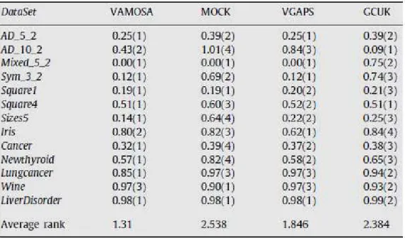
4.1 Rankings (in brackets) for algorithms VAMOSA, MOCK, VGAPS

and GCUK over 13 datasets, based on the MS value obtained 71

4.2 Median values of adjusted Rand index for articial and real data

sets 79

4.3 Rankings for K-means, GAPS, GAnPS, EM and AL over 21 da-ta sets, based on the Minkowski Score (MS). The best MS values are

marked in bold 83

6.1 16 scenarios depending onω, K, D¯ . A comparison of Mclust and

Kmeans according toSBI. Sc stands for Scenarios 121

6.2 16 scenarios depending onω, K, D¯ . Performance of Mclust

con-ditionally toSBIM candSBIt. Sc stands for Scenarios 121

6.3 Performances of M clust and Sbam in terms of ACAE and

ARAN D 126

6.4 Performances of M clust and Sbam in terms of ACAE and

(10)

7.1 Performance of Mclust and Sbam in real data examples without

implementingSBI−d 139

7.2 Performance of Mclust and Sbam in real data examples

(11)

Introduction

Partitive clustering methods represent one of the earlier and most famous sets of strategy in the field of clustering. The name comes from their main feature: all these methods start from an initial partition and modify it at every step of the pro-cess according to a known criterion, until a given convergence rule is satisfied. In other words, as pointed out by Äyrämö and Kärkkäinen (2006), they work essen-tially as iterative allocation algorithms. In this framework, we do not only focus on “canonical” approaches such as K-means and fuzzy C-means, but discuss some recent symmetry-based partitive clustering methods, mostly developed in the con-text of computer science and engineering. As it will be shown, these approaches seem to provide encouraging results, especially in the field of image recognition and some related applications, and for this reason, they represent a starting point for our work.

In this respect, we are particularly interested in the case of overlapping clusters. As we will clarify, this case may represent a critical aspect for most clustering meth-ods we have considered. In particular, we started our analysis by noting that, in a case of high-dimensional data with overlapping clusters, it may be difficult to choose the component-specific distributions, and no graphical device can help us. So, we decided to investigate non parametric approaches to clustering. In this framework, we focused on the case of clusters with elliptical shapes, and in Gaussian mixtures as a special case. Then, we realized that for elliptical shapes the symmetry could be a “natural” choice. So, we searched for such clustering approaches, and we found the symmetry-based methods cited above. But, surprisingly, none of them was in-tended to focus on elliptical clusters, since their aim is essentially at handling image recognition of different symmetric shapes. So, we decided to discuss this issue, and to test whether a suitable function of symmetry could improve clustering results in the case of elliptical overlapping clusters.

Since we are interested in elliptical shapes, from a clustering point of view, an-other broad subject that we will discuss is the Gaussian mixture model. This ap-proach, whose starting point is commonly identified in Pearson (1894), has known an increasing interest, especially from the second half of the past century, due essen-tially to the EM algorithm, see Dempster, Laird and Rubin (1977). In this context, our interest is in the EM-based Mclust algorithm from the R library mclust, see Fraley and Raftery (1999).

Thus, our work addresses both of these topics, partitive clustering methods (with a focus on the symmetry-based approach) and Gaussian model-based clustering.

(12)

2 The main reason of such a choice, that is to address two partially different sub-jects, derives from the essential features of our proposal: a symmetry-based parti-tive method which is intended to deal with elliptical clusters (with Gaussian being a special case). In this sense, we provide an evaluation of our clustering perfor-mances by proposing a comparison with the Gaussian mixture model implemented in the Mclustlibrary. This is surely a challenging task, since this method has home-court advantage in the case of Gaussian clusters. In this framework, as pointed out before, we are mainly interested in the case of overlapping clusters. In this sense, a starting point for our work was the assumption thatM clust(also in its “natural” framework, that is Gaussian mixtures) could have problems in centroid estimation when clusters are highly overlapped. Quite obviously, this drawback could be re-lated to its dependency on the mutivariate Gaussian density. So, we searched for a non parametric skewness-based method, which could be appropriate for ellipti-cal distributions (including Gaussian) in the case of overlapping clusters. This was exactly the framework of the proposed Sbam (Skewness-Based Allocation Method) algorithm.

The outline of this work is the following.

In Chapter 1, we briefly present the framework of clustering and introduce some related notions and definitions in a basic way. We discuss the main issue addressed in our work, namely the case of overlapping clusters (with some graphical repre-sentations), with a brief view on the possible consequences of such a case on the clustering results. Finally, we introduce the related concept of intersecting areas (which we use to provide a definition of the overlapping regions) and the idea of our proposal: to develop a skewness-based clustering method dealing with elliptical overlapping clusters.

Chapter 2 deals with most used partitive clustering methods, namely the K-means in the versions of Forgy (1965) and MacQueen (1967), the Fuzzy C-means, see Dunn (1973) and Bezdek (1973), and the K-medoids methods, e.g. PAM and

CLARA, see Kaufman and Rousseeuw (1987,1990) respectively and CLARANS, see e.g. Ng and Han (2002). In this framework, the concept of point prototype-based clustering has a key role. According to Xiao and Yu (2012) “partitional clustering algorithms suppose that the data set can be represented by a set of prototypes, there-fore is also called prototype-based clustering method ... According to different defi-nitions of prototypes, prototype-based clustering methods can be widely categorized into two groups: point-prototype-based clustering algorithms and prototype-based clustering algorithms using non-point prototypes, such as line, hyperplane, and hy-persphere, generally called non-point-prototype-based clustering algorithms”. Es-sentially point-prototype-based clustering defines cluster as a set represented by a

(13)

3 point in the space of the observational features (e.g. mean or median or medoid). All of the methods considered in this Chapter are presented as point prototype-based approaches, with the further distinction into two types: virtualpoint prototype clus-tering and actual data point prototype clustering. Roughly speaking, virtual point prototype clustering do not belong to the original dataset (such as mean), while

actual data point do (e.g. medoids). So, according to this formulation, we discuss the K-means and the Fuzzy C-means as virtual point prototype methods, while the

K-medoid approaches are interpreted asactualpoint prototype methods.

In Chapter 3, we discuss the model based approach to clustering, focusing on Gaussian Finite Mixture Models. To this end, a first subsection is dedicated to Finite Mixture Models, with a brief history and some basic definitions. The sec-ond paragraph discusses Finite Mixture Models in a clustering framework; a further section deals with Finite Mixture Models and the related maximum likelihood ap-proach to parameter estimation. In this context, we consider the EM ( Expectation-Maximisation) algorithm to estimate mixture parameters. Finally, we discuss a spe-cific implementation of the EM algorithm for the Gaussian case, included in the R

M clust library, looking to constraints on the component-specific covariance matri-ces. This last subsection is relevant, becauseM clustis one of the reference methods for clustering based on Gaussian mixtures, and it will be the direct competitor of the method proposed in the following Chapter 5.

In Chapter 4, we present some recent contributes to symmetry-based partitive clustering methods. These have been mostly developed in the context of computer science and engineering. All of them are not involved with specifical statistical hypotheses (e.g. assumptions on model structure), but rather aim at identifying symmetric shaped clusters. So, from a statistical point of view, they do not repre-sent parametric approaches. The aim of this section is to provide a short literature review on the skewness-based approaches and to illustrate some drawbacks con-nected to the use of symmetry in the clustering framework. This section is relevant for at least two reasons: first, the analysis of the drawbacks related to the use of symmetry functions helped us in the formulation of our proposal. Second, the pro-posed skewness-based method can be considered as an evolution of the algorithm in Su and Chou (2001), discussed at length in the literature review.

In Chapter 5, we present a novel skewness-based clustering method. A source of inspiration for this method could be found in the papers we have discussed in Chapter 4. The results obtained by those approaches suggest that skewness-based techniques may represent a rapidly increasing and promising field of research. In

(14)

4 particular, they have very good performance when compared to other, recently de-veloped, clustering methods. Nevertheless, there are some relevant differences be-tween the proposed method and the skewness-based approaches presented in Chap-ter 4. First of all, the field of application: all the clusChap-tering techniques discussed have been defined and implemented in a non parametric context, while the pro-posed method is specifically introduced in a model based clustering framework (we are primarily interested in Gaussian mixtures). Only the case of Gaussian densities is explicitly considered, even though in this Chapter we suggest some extensions of the proposed method to elliptical distributions. This fact leads us to a further, non-negligible, difference: despite the generality of the prevoius approaches (they work well with clusters having a different shape), we focus on a particular cluster shape, the elliptical one, which may be associated to the general class of elliptical distributions. This means that our method could not be appropriate when the target is a different kind of clustering. The main features of the proposed method are ex-plained throughout this Chapter, which is organized as follows. In the first section, we give a look at the case of overlapping clusters, and discuss why the proposed method could be appropriate when other competitors fail. Then, we introduce a skewness function, and a related skewness-based index(SBI), adopted as a cluster validation index. In the third section, we define and discuss the objective function and give a sketch of the corresponding algorithm, followed by some remarks on the differences with respect to other skewness-based methods. In the last section, on the basis of Dvoretzky’s Theorem (1961), we provide a further support to the search of elliptical clusters, beyond the assumption of an elliptical distribution, and we suggest a further direction of development for the proposed method.

Chapter 6 is devoted to the empirical evaluation of our proposal. In this sense, we provide an analysis of the clustering performances in two different simulation studies: the first one deals with the skewness-based cluster validation index (SBI), while the second involves a comparison between the function M clustand the pro-posedSbam(Skewness-Based Allocation Method). We consider Gaussian mixtures in several different clustering scenarios, where the clustering complexity (associated to the overlapping degree) is under control. To this end, the outline of the Chap-ter follows: in the first section, we introduce the theorical definition of overlapping clusters degree, on the basis of Maitra and Melnykov (2010), and the M ixSim function which generates different Gaussian mixtures according to a value of over-lapping degree, as developed in Melnykov, Chen and Maitra (2012). In this context, we also provide some bivariate graphical examples to illustrate the potentials of this generator. In the second part, we introduce the definition of absolute error when estimating the cluster centroids (centroid absolute error,CAE), and we discuss the

(15)

5 performance of the skewness-based cluster validation index(SBI) in different sim-ulation scenarios. Finally, we provide a comparison between M clust and Sbam in terms of clustering performances, in several different clustering scenarios, with some concluding remarks.

In chapter 7, we discuss some applications of the proposed skewness-based al-gorithm in a real data framework. In this sense, we stress the fact that a single real data set, although highly representative of some interesting features, is still a single one, thus being less informative when compared to the virtually infinite possibilities provided by simulations. We stress as well the fact that the analysis of real data examples can be instructive in a further sense. For instance, taking real data ex-amples may help analyze the behaviour of the proposed clustering method under a potentially misspecified model, that is when we do not know whether clusters come from a Gaussian mixture. This is the main reason of the Chapter.

In the first section, we briefly introduce the real data sets considered, focusing only on their basic features (names, year of reference and relative sources). In further subsections we provide a more detailed description of the same data sets, togheter with the performances achieved by theM clustfunction and the proposed Sbam for each dataset, in terms ofCAE, SBI and adjusted Rand Index. Then, we propose an extended, albeit absolutely tentative, version of Sbamwhich we test on the same real data examples. Finally, we conclude with some remarks about the performance of the two clustering methods on the real data considered, and some proposals for further developments.

(16)

Chapter 1 Some clustering problems and the issue of overlapping clusters

In this section, we briefly introduce the framework of clustering and present some related definitions in a basic way. Then, we move to the main issue addressed in our work, namely the case of overlapping clusters (see below for a graphical representation), with a brief discussion on the possible consequences on the clus-tering results provided by different approaches. Finally, we introduce the related concept of “overlapping regions” and the idea underlying our proposal: to develop a skewness-based clustering method dealing with overlapping clusters.

1.1 The notion of cluster

There is not a unique problem in the framework of clustering, but many different problems. Roughly speaking, clustering techniques aims at associating group to a set of objects. But what is a cluster? A group of objects that are more similar to one another than to members of other clusters? Or a group of objects that are more dissimilar to members of other clusters than to one another? And what do we mean by similar/dissimilar? These seemingly simple questions lay at the heart of the matter: in fact, an objective and univoque answer does rarely exist. It strongly depends on several factors: the specific field we are involved in, the aim of the researcher, and so on. For instance, if our aim is to group some words to form real and meaningful sentences (clusters), the corresponding definition of cluster will be quite different from that of a doctor who wants to group patients on the basis of their blood pressure levels. Even in the same clustering framework, we could well be interested in different kind of clusters: patients with a similar overall pressure (i.e. similar means) or patients with similar changes in blood pressure (i.e. similar variances).

Furthermore, nothing has yet been said about how many clusters we are looking for in the data. Is this inherent to the nature of data, or it depends rather on the specific interest of the researcher? Probably, the best answer to these questions may

(17)

1.2 NOTATION

7 be found in the words of Estivill-Castro (2002): “Do not forget that clusters are, in large part, on the eye of the beholder”. In short, these are only a few aspects out of those that help to make clustering a quite challenging and uncertain task.

1.2 Notation

To put it formally, let us consider a dataset consisting of n multidimensional pointsX= (x1, x2, ..., xn)drawn from a setS and let us suppose that our aim is to

buildKdisjoint subsets based onX, sayS1, S2, ..., SK, so that fori6=j = 1,2, ..., K the following conditions hold:

Si∩Sj =Ø

S1∪S2∪...∪SK =S

Therefore, the result will be a partition{S1, S2, ..., SK}of the original dataset. The subscript is often referred to as label, so that all the data points belonging to cluster Sk, will have the same labelk, andK labels will be available in all. In addition, we represent the cardinality of thek-th cluster as|Sk|.

So, assuming |Sk| > 0 for every k, and forgetting observations’ order within a cluster, for fixed n and K (n _> K) we may have 1

K! PK i=0(−1) K−i K i in _different partitions (Stirling number of the second kind). But how to decide whether a partic-ular solution is a sensible one? There is, indeed, a plethora of different criterions, each corresponding to different aims and/or contexts of the adopted clustering pro-cedure. As pointed out by Hennig et al. (2016), “the reader should be aware that clustering, or grouping of data, can mean different things in different contexts, as well as in different areas of data analysis. There is no unique definition of what a cluster is, or what the “best” clustering ... should be. Hence, the cornerstone of any rigorous cluster analysis is an appropriate and clear definition of what a “good” clustering is in the specific context”. It is quite evident, therefore, that there is no silver bullet when a clustering framework is considered.

It is also quite complex to classify the different paradigms and methods used for clustering; as an index of to topic, note that Murtagh and Kurtz (2016) found more than 404.000 contributions to the clustering literature. Here, we focus only on partitive clustering methods and Gaussian mixture models, see Chapter 2 and 3, respectively. For a short list of the main elements of a cluster analysis it is possibile to cite the following structure from Äyrämö and Kärkkäinen (2006):

1. Data presentation. 2. Choice of objects.

(18)

1.3 OVERLAPPING CLUSTERS

8 3. Choice of variables.

4. What to cluster: data units or variables. 5. Normalization of variables.

6. Choice of (dis)similarity measures.

7. Choice of clustering criterion (objective function). 8. Choice of missing data strategy.

9. Algorithms and computer implementation (e.g. convergence) 10. Number of clusters.

11. Interpretation of results.

For each of these points (and their combinations) we may choose different strate-gies, and this partially clarifies the extent of the issue. For a detailed discussion of different clustering paradigms see Hennig et al. (2016).

1.3 Overlapping clusters

Our focus here is on partitive clustering methods and, in particular, on model based clustering via Gaussian mixture models (they will be discussed in Chapter 2 and 3, respectively). Within this framework, the main scope is a sensible estimation of clusters centroids, intuitively defined as the barycenters of the corresponding clusters and obtained as the “central position” of all the points, when all of the coordinate directions are considered.

Generally speaking, one of the main issue in this context, is related to the pres-ence of anomalous data which may alter in some way the structure of the clusters (the underlying distributions in the case of Gaussian mixture models). This type of data is commonly known as outliers or contaminating points. Actually, a cluster may be contaminated in many different ways, each one leading to a different kind of outliers. Thus, there are many possibilities for defining what we mean by outlying point. Very basically put, we can distinguish at least the following:

1. Extreme values. Data points which show values much larger (or smaller) with respect to the other ones. Clearly, in a multivariate framework, this may occur relatively to one or more dimensions.

2. Leverage points. Points that show an abnormal “behaviour” with respect to the others; just to give an example in the bivariate case, an extreme value showing a departure from the “usual” relation between the two coordinates. In the regression framework, for instance, this can crucially affect the intercept and slope estimate. 3. Bridge points. Data points which identify a region of intersection between two or more clusters.

(19)

1.3 OVERLAPPING CLUSTERS

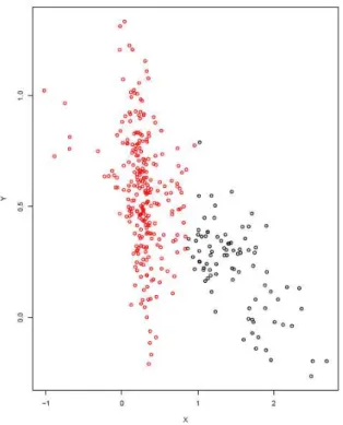
9 To handle these cases, many different robust clustering methods have been de-veloped, see Chapter 2 for a brief list of some recent approaches.

Our work is not involved with such methods and related problems. Nonetheless, for our purpose the case of bridge points is a crucial issue. In fact, we are mostly interested in studying the overlapping clusters, which naturally determine the pres-ence ofbridge points. In this sense, it is possible to represent at least four different scenarios of increasing overlapping degree, which is depicted in the following Fig-ure:

(a) (b)

(c) (d)

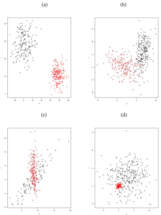
Fig. 1.1: Two clusters with increasing degree of overlap. (a) Well separated clusters, (b) low degree of overlap, (c) medium degree of overlap, (d) high degree of overlap

(20)

1.3 OVERLAPPING CLUSTERS

10 In the first case, Fig. 1(a), clusters are clearly well separated, and the overlap does not occur, so that a good allocation of points as well as a proper estimates for the centroids are quite naturally obtained.

In the second case, Fig. 1(b), clusters are not well separated, and some overlap does occur in the tail of the “black” cluster. This case is somewhat complex for the estimation of centroids. In fact, if even only few points in the overlapping region were assigned to the red cluster, the estimate of the centroid of the black cluster would be seriously biased. In fact, those few points lying at the extreme tail of the black cluster, are essential to a proper estimate of the corresponding centroid.

In the third case, Fig. 1(c), clusters are even more overlapping. In this case, there is a high risk of misclassification of a relevant number of data points, due to the quite substancial overlapping area. In this sense, it is interesting to stress the difference between case (b) and (c). Let us suppose that, in both cases, all of the points in the overlapping regions are assigned only to the red cluster, and assume that all the other points would be exactly allocated in the corresponding clusters. So, in case (b) we would obtain a severe bias in the centroid estimate of the black cluster but a little rate of misclassification (due to a fewbridge points), whereas in case (c) we would have the opposite situation: a certain bias (not necessarily negligible, but possibly lower than previous one) in the centroid estimate of the black cluster, but a significant rate of misclassification (due to the overlapping area).

In the last case, Fig. 1(d), we have totally overlapping clusters, a sort of innested clusters (but not in a hierarchical sense). In this case, provided that our clustering method would be able to detect the nested cluster (really not a trivial matter), it is easy to expect a strong bias in the centroid estimates as well as a significant rate of misclassification. This last case, which could seem a somewhat extreme and un-realistic case, can actually be explained in the following way. Let us consider a bidimensional data set with blood pressure and heartbeat measures for two clus-ter of hypertensive and tachycardic patients. Suppose one of the two clusclus-ters (the nested one) is composed by subjects treated with a particular drug against hyper-tension and tachycardia, while the other cluster is composed by untreated subjects. If the drug had the further feature of reducing the variability in both blood pressure and heart rate, we would be in a scenario quite similar to that shown in Fig. 1(d). In fact, we would have a smaller cluster (due to the reduced variability in both dimen-sions), and a centroid located down and to the left (due to the lower blood pressure and heartbeat) with respect to the bigger cluster.

It is worth noting that also the other overlapping cases depicted in Figure 1, namely (b) and (c), are liable to analogous explanation. In this sense, in all of the

(21)

1.4 OVERLAPPING REGIONS AND A SKEWNESS-BASED PROPOSAL

11 overlapping cases we have considered,bridge pointsdo not really alter the structure of the real clusters involved, but rather reflect a sensible intersection of the clus-ters. If anything, in these casesbridge pointsalter the structure of the clusters which probably our methods are able to detect. In other words, they must not be neces-sarily considered as outliers, but they can be seen as “standard” points, determined by an overall overlapping context, depending on different but sensible causes (like those just discussed). From this point of view, with respect to the three type of out-liers considered above, onlyextreme valuesandleverage pointswill be interpreted as outliers, because both alter the real structure we expect to detect in a cluster.

Finally, note that there is a relationship between the overlapping degree and the rate of misclassification depicted in the four sub-figures. In fact, it is even possible to define a sort of clustering complexity degree (related to the lack of separation between clusters) in terms of misclassification probabilities, in a way that will be addressed in Chapter 5, according to Maitra and Melnykov (2010). So, the above considerations on misclassification in case of overlapping clusters will find a natural explanation, which links the complexity of a clustering scenario with its overlapping degree, showing the centrality of this issue.

1.4 Overlapping regions and a skewness-based proposal

Here, we want to point out that, in the above overlapping cases, all the issues re-lated to bias in centroids estimates and misclassification of points can be traced back to the role of the distance that usually involved in partitional clustering methods. In fact, in Fig. 1, (b)-(d), none of the common distance-based methods will be able to assign bridge points to the proper cluster; in fact, whatever the type of distance we choose, those points will be allocated to the nearest centroid, which can lead to a wrong assignment (in the case of Fig. 1(b) this is more than a simple possibility). From this point of view, it can be noticed that also Gussian mixture approach to clus-tering may be interpreted as a distance-based method, since the likelihood value is based on a particular “kernel distance”, depending on some parameters we want to estimate. In other words (and roughly speaking) the maximum likelihood approach can be regarded as a distance-based method, which aims at finding centroids mini-mizing the sum of “kernel distances” of data points to the corresponding centroids. Thus, as we will see in Chapters 5, also the Gussian mixture approach to cluster-ing may suffer from the same limitations in case of overlappcluster-ing clusters (although

(22)

1.4 OVERLAPPING REGIONS AND A SKEWNESS-BASED PROPOSAL

12 it may outperform other clustering methods). So, once we have chosen a specific metric distance, we can not avoid the potential issue of overlapping clusters and we can only expect that in such cases shapes as well as cluster centroid estimates will not be altered too much.

Note that this is not a trivial matter, as in presence ofbridge pointseither partitive clustering methods or Gussian mixture model-based clustering suffer from bias in allocation and centroid estimates (for a brief discussion of these methods see Chap-ters 2 and 3, respectively). One of the most important clustering approach which can be adopted in such cases is theFuzzy C-means, see Dunn (1973), which will be discribed in Chapter 2.

Here, we would just notice that the solution to the problem of overlapping clus-ters provided by Fuzzy C-means is not the only possible solution. In particular, as we will clarify in Chapter 2, fuzzy solutions, even in the best case, are not able to reproduce the true underlying partition. To achieve this aim, a clustering method should be able to detect and reproduce the overlapping regions.

Beyond the intuitive meaning of overlapping clusters provided in Fig. 1.1, it is also possible to formalize it. For this purpose, we need first to introduce the concept of intersecting area and the related convex hull of a set. This is, roughly speaking, the smallest convex set containing all the elements of the originary set, see the following figure, which depicts a simple bidimensional example:

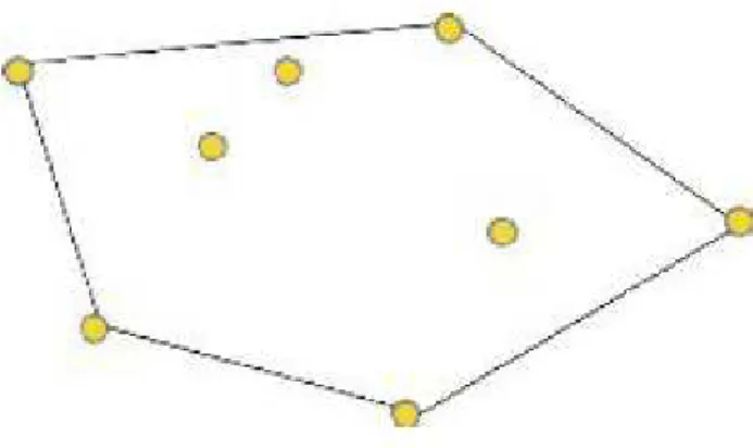
Fig. 1.2: Bidimensional convex hull

As depicted in Fig. 2, the convex hull of the set of yellow points is the set ofall the points in the pentagon-type area (not only the yellow ones).

(23)

1.4 OVERLAPPING REGIONS AND A SKEWNESS-BASED PROPOSAL

13 Now, letCSk be the convex hull defined on points belonging to clusterk. Thus, for two clusters, say k and k0, the intersecting area Ikk0 can be defined as the

in-tersection of the convex hulls of the corresponding clusters, such that the same intersection is not a null set, that is

Ikk0 =C_S

k ∩CSk0|CSk ∩CSk0 6=Ø

An intuitive example of this formulation can be found in Fig. 1.1(c), where the graphical intersection between the two clusters is particularly evident. But, clearly the formulation includes all possible cases, a part from those where intersection does not occur, as in Fig. 1.1(a). The same definition has an obvious extension to an arbitrary number of clusters involved in the same intersecting area, i.e. Ikk0_k00

will indicate a three clusters intersection, for distinct values ofk,k0 andk00.

Now, to introduce the concept of overlapping region, we refer to the aforemen-tioned intersecting area. In fact, the overlapping region is a particular case of intersecting area, when there are points in the region that belong to each of the intersecting clusters, as in the following figure:

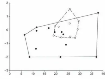
Fig. 1.3. Bidimensional overlapping region

where the dotted lines is used only to distinguish between the two clusters (while theoretically convex hulls can not be represented by such lines). Note that both clusters have at least one element in the intersecting area (empty dots and black dots, respectively), such that this intersecting area is also an overlapping region. Clearly, this is the real partition. If our clustering method misclassified the three black dots in the overlapping region, assigning them to the empty dots cluster, it

(24)

1.4 OVERLAPPING REGIONS AND A SKEWNESS-BASED PROPOSAL

14 would reproduce an intersecting area, because black dots cluster would not have any element in the intersecting area.

To put it formally, in the case of two cluster, say k and k0 with corresponding elementsi∈Skand j ∈Sk0, the overlapping regionOR_kk0 can be defined as

ORkk0 ={I_kk0| ∃ (i∈S_k, j ∈S_k0)∈I_kk0}

Note that, by this way, we retain the hypothesis of null intersection between clusters considered as set of points, that is k 6= k0 Sk ∩Sk0 =Ø k, k0 = 1, ..., K. In

fact, the overlapping regions are regions containing points in two or more clusters, where each point belongs to one and only one cluster.

This is the so-called hard partition, as opposite to the fuzzy assignment proce-dure, where each point may belong to more than one cluster, as in the Fuzzy logic, see Chapter 2 for a discussion. Here, what we intend to stress is the fact that in the case of bridge points overlapping regions may be present in the true partition, whereasfuzzy“partition” may be just an abstract structure built to avoid bias in cen-troids estimation. In other words, a partition with overlapping regions may reflect thetruepartition we are looking for, while thefuzzy partition do not.

Thus, the ideal would be a method to catch and handle the overlapping regions, while based on a suitable notion of distance. But the issue of detecting overlapping regions is not a trivial one. In fact, for the same reason discussed above, such a task can not be achieved by none of the methods entirely based on metric distance: with two or more centroids and a point in a overlapping region, not only this point but also all the other points in a suitable neighborhood of the same point will be as-signed to the nearest centroid (in the sense of the choosen distance), thus vanishing the possibility of detecting overlapping regions.

In other words, all of the mehods, based on a distance only, will induce a parti-tion in the sense of clusters, that is a partiparti-tion in the correspondingD-dimensional space, while overlapping regions do not fulfill this assumption. From this point of view, to handle the overlapping regions and to allow for a suitable notion of dis-tance are two different tasks which could be in conflict: the first aim may not be achievable while pursuing the second.

This complex scenario is the starting point of our proposal: to combine a distance approach with another procedure (based on symmetry) to counterbalance these drawbacks. In this context, our work is intended to study howbridge pointsinfluence centroid estimates in the case of Gaussian clusters, and to propose a skewness-based method to improve these estimates. In this sense, we expect symmetry to

(25)

1.4 OVERLAPPING REGIONS AND A SKEWNESS-BASED PROPOSAL

15 show two particular features at the same time: to detect Gaussian-shape clusters while improving allocation of the points in overlapping regions. The comparison in clustering results will be done with respect to the Gussian mixture approach as implemented by the Mclust algorithm (see Chapter 3 for details). In the case of Gaussian clusters, this is surely a challenging task, because Gussian mixture models reflect the underlying “truth”.

(26)

Chapter 2 Prototype-based methods

Partitional clustering methods represent one of the earlier and most famous set of techniques in the clustering history. The name comes from their main feature: these methods start from an initial partition and modify it at each step of the pro-cess according to some criterion, until a given convergence rule is satisfied. In other words, they work essentially as an iterative relocation algorithm. According to Äyrämö and Kärkkäinen (2006), we can describe a general partitive clustering method as follows:

Input: The number of clustersK, and a database Xcontainingnobjects in_RD Output: A set ofK clusters, which minimizes a criterion functionQ (X, K). Step 1. Begin with initialK centers/prototypes as the initial solution.

Step 2. (Re)compute memberships for the data points using the current cluster centers.

Step 3. Update some/all cluster centers/prototypes according to the updated membersips of the data points.

Step 4. Repeat Step 2-3 until no convergence in terms of Q (X, K)or no data point changes cluster membership.

In this general context, partitional clustering methods aim at estimating cluster centers, which denote representative quantities for the clusters. To this end, not only the mean, but also the medoid (an element of the cluster as a representative member) represents a typical choice. The best-known strategies in this sense are, re-spectively, theK-meansand the more robustK-medoids(this one exploiting medoid, an element of the cluster as a representative member, rather than mean).

From this point of view, it is possible to distinguish between different partitional clustering algorithms on the basis of the quantities choosen as representative, which often are referred to as prototypes, as detailed in Xiao and Yu (2012): “Generally, partitional clustering algorithms suppose that the data set can be represented by a set of prototypes, therefore is also called prototype-based clustering method ... Ac-cording to different definitions of prototypes, prototype-based clustering methhods

(27)

2.1. VIRTUAL POINT PROTOTYPE-BASED METHODS

17 can be widely categorized into two groups: point-prototype-based clustering algo-rithms and prototype-based clustering algoalgo-rithms using non-point prototypes, such as line, hyperplane, and hypersphere, generally called non-point-prototype-based clustering algorithms”.

In the next, we will focus on point prototype-based clustering algorithms, be-cause they are likely the most commonly use, and above all, our proposal is also point-prototype-based.

Essentially, point-prototype-based clustering defines cluster as a set represented by a point in the space of the features. In this sense, point prototype clustering methods may be distinguished into two types: “virtual” point prototype clustering and “actual” data point prototype clustering. Roughly speaking, prototypes in vir-tual point prototype clustering techniques do not necessarily belong to the original dataset, while prototypes inactualdata point prototype clustering do. For instance, if we choose means as cluster prototypes, these will not be in the original dataset (apart from special cases, e.g. if a cluster contains only one observation, this will obviously coincide with the corresponding mean). So, in the following, we will first discuss virtual point prototype clustering methods and then proceed to the actual prototype clustering methods.

2.1. Virtual point prototype-based methods

The underlying idea of virtual point prototype clustering methods is essentially to minimize a given objective function, with each cluster represented by a virtual point prototype. Basically, it is possible to define a generic objective function as follows Q (X, K) = K X k=1 n X i=1 wikkxi −mkkp

where wik ∈ {0,1} denotes the membership value (boolean) of a data point i to cluster k, mk is the prototype relative to that cluster k, the superscript p is the power used for the distance between the obserbationxi and thek-th prototypemk. Clearly, many different manipulations of the objective function are also possible, see below for details. Among the earliest partitional clustering algorithms we can find theK-means, see Forgy (1965) and MacQueen (1967), which is a typical virtual point prototype based clustering approach, based on means as cluster prototypes,

(28)

2.1.1. K-MEANS

18 i.e. mk =x¯k. In the next, we discuss the main aspects of this method and some of

its variants.

2.1.1. K-means

Essentially,K-meansis an iterative method that aims at splitting a dataset intoK disjoint groups. K-meanschooses the cluster means as ptototypes and the Euclidean distance as a measure of dissimilarity, i.e. mk = x¯k and p = 2. Perhaps, its main

distinctive feature is the objective function, which is based on the within-cluster squared error. This both measures the quality of the clustering result and rules the allocation process. Formally, in the case of a D-dimensional dataset, and a sample includingnpointsxi ∈RD,i= 1, ..., nand for a choice of the number of clusterK, the criterion to be minimized is

Q (X, K) = K X k=1 n X i=1 wikkxi−mkk2

In the previous expression Pn

i=1wik = P

i∈Sk, where Sk is the set of points as-signed to the kth cluster, andmk = x¯k is the centroid of thekth cluster. Note that

the equality mk = x¯k holds since, conditionally to a given partition, the aritmetic

mean is a minimizer of the corresponding cluster within deviance (as it defines the center of order 2), and the sum of minima over Sk guarantees the total minimum for the objective function. So, in matrix notation, the above criterion corresponds to minimize PK

k=1trace (Wk), where Wk is the covariance matrix for thekth cluster. In fact, the trace of a (square) matrix is the sum of its diagonal elements, i.e. in the case of Wk the variances for each dimension. The D-dimensional point which minimizestrace (Wk)corresponds to the Daritmetic meansx¯k, and the expressions

above coincide.

In this sense, K-meansis also referred to as a variance minimization technique, see Kaufman and Rousseeuw (1990). Before the “official” K-means was proposed by Forgy (1965) and MacQueen (1967), a similar criterion was proposed by Ward (1963), in a hierarchical rather than a partitive context.

Hereafter a sketch of the K-means algorithm in the version described by Forgy (1965), for a dataset containingn objectsxi ∈RD,i= 1, ..., nis given

(29)

2.1.1. K-MEANS

19 Input: Choose a number of clusters, sayK

Step 1. randomly initializeK centroidsx¯k∈RD

Step 2. for i= 1, ..., n,

allocatexi to thekth cluster according to the following criterion wik = 1 if k = arg min

k kxi−x¯kk

Step 3. Update centroidsx¯k according to the newwik, with a cluster cardinality equal to|Sk|, do fork = 1, ..., K, fori= 1, ..., n ¯ xk = Pn i=1wikxi Pn i=1wik = P i∈Skxi |Sk|

Step 4. Repeat Step 2-3 until no data point ichanges cluster membersip. Output: A set ofK clusters, which (locally) minimizes the objective function

Q (x¯k;x) = K X k=1 X i∈Sk kxi−x¯kk 2

TheK-meansis a greedy algorithm, that is at every run it produces the maximum decrease in the objective function Q (x¯k;x), until it converges to a local minimum,

see Jain (2010).

Actually, the same K-means criterion encompasses both strenghts and weak-nesses. In fact, inducing compact clusters (i.e. with a low within-cluster variability) makes interpretability easier (highly homogeneous elements in each cluster). On the other hand, it fails every timetrueclusters are somewhat similar (i.e. not well-separated centroids and/or high variances, see further discussion in Chapter 4). The choice of the euclidean norm in the objective function makes clustering results sen-sitive to extreme values, so that the process shows a low level of robustness. The choice of medoids rather than means in theK-medoids, see Kaufman and Rousseeuw (1987), is intented to balance this drawback. Paragraph 2.1.1.2 is devoted to discuss in more details some of these drawbacks.

However, its implementational simplicity and computational efficiency makes it a still actual and popular clustering method. For the same reasons, it has been con-sidered as an initialization technique for other computationally expensive methods, see e.g. Bradley and Fayyad (1998). Finally, K-means type algorithms have been

(30)

2.1.1.1. VARIANTS OF THE K-MEANS METHOD

20 developed in a wide number of variants, the main of which are presented in the following.

2.1.1.1. Variants of the K-means method

Before the “official” release of theK-meansmetod, described by Forgy (1965) and MacQueen (1967), two early works, which are strictly related to those, have been introduced by Fisher (1958) and Lloyd (1957, 1982). As outlined in Äyrämö and Kärkkäinen (2006) “K-meanstype grouping has a long history. For instance, already in 1958, Fisher investigated this problem in one-dimensional case as a grouping problem”, and even earlier, “Lloyd presented a quantization algorithms for pulse-code modulation (PCM) of analog signals. The algorithm is often referred to as Lloyd’s algorithm and it is actually equivalent with the Forgy’sK-meansalgorithm in a scalar case”. Although Lloyd’s paper was not published before 1982, the unpub-lished manuscript from 1957 is referred, for example, by Chen (1977) and Lindeet al. (1980), respectively.

However, the first versions of theK-meansmethod were published independently by Forgy (1965) and MacQueen (1967). There are two main differences between the two formulations:

1. Allocation step. In Forgy (1965), cluster centers are updated only after all

observations are allocated to the closest centroid, while in the MacQueen (1967) release the centroids are updated every time a single data point is assigned to a cluster (clearly only the two clusters involved will be updated, i.e. the cluster which “looses” his data point and the one which “gains” it).

2. Convergence. In Forgy (1965) the algorithm runs until convergence is reached, generally in a time proportional toO(nDKt)wheretis the number of iter-ations, see Duda et al. (2001). Vattani (2011) showed that K-meansmay converge in an exponential time “even in the plane”. In the release by MacQueen (1967) the basic algorithm runs only one time (until all data points are allocated to the K clusters, so that there’s no iteration, see Äyrämö and Kärkkäinen (2006)). These features ofK-meansalgorithms will also be addressed within the framework of our proposal, see Chapter 5.

(31)

2.1.1.2. DRAWBACKS OF THE K-MEANS

21

2.1.1.2. Drawbacks of the K-means

As we noted before, the different versions of the K-meansalgorithm have some drawbacks that helped to kick-start new variants that have been developed in the last decades; for a review see e.g. Äyrämö and Kärkkäinen (2006). Among the most well known drawbacks we may recall:

DRAWBACKS RELATED TO THE ALGORITHM

1. Sensitivity to initial configuration. The basic algorithms are local search heuris-tics and the K-means cost function is non-convex; therefore the algorithm is very sensitive to the initial configuration and the resulting partition is often only subop-timal.

2. Order-dependency. The MacQueen’s basic and converging variants are sensi-tive to the order in which the points are relocated. This is not the case for the batch versions (such as Forgy’s one).

3. Empty clusters. The Forgy’s batch version may lead to empty clusters due to poor initialization (while in MacQueen’s formulation this usually does not occur; if the process leads to a cluster with a single observation, it would coincide with the mean, thus necessary remaining in the same cluster).

DRAWBACKS RELATED TO THE METHOD

4. Lack of robustness. The sample mean and variance are very sensitive to outliers. So-called breakdown point for the mean is zero (roughly speaking, the breakdown point is the proportion of outlying observations, which an estimator can handle before giving an incorrect result). This means that even only one huge error may completely bias the estimate. The obvious consequence is that the K-means

method is highly non-robust as well.

5. Unknown number of clusters. SinceK-meansis in general a “non-hierarchical” method, it does not provide any information about the number of clusters, in the sense it is started for given and fixed K. However, it is possible to develop ad-hoc

procedures to choose the optimal number of clusters. See, for instance, Hamerly and Elkan (2004).

6. Only spherical clusters. K-means is based on spherical components/clusters. Therefore, a large amount of “clean” data is usually needed for successful clustering. 7. Handling of nominal values. The sample mean is not defined for nominal values. To solve this issue several variants for the original versions have been devel-oped.

8. Hard membership values. The membership values in the K-means functions are “hard” in that they may assume only two values, 0 or1, since each data point can be assigned only to a single cluster (the so-called hard assignment). According

(32)

2.1.1.2. DRAWBACKS OF THE K-MEANS

22 to Xiao and Yu (2012), this drawback makes the K-meansmethod not applicable to complex datasets which contain overlapping clusters or some data points that can not be easily allocated to one cluster.

Actually, the real problem with overlapping clusters, in our opinion is not due to thehard assignmentstrategy, but rather to the objective function itself. In this sense, it seems hard to suppose that a distance based criterion can be suitable for the case of overlapping clusters. To catch this issue, let us consider the simple case of two clusters (K = 2) for a bidimensional dataset, as depicted in the following figure:

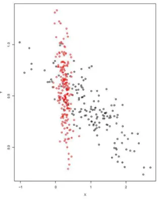
Fig. 2.1: Overlapping on a tail (truepartition)

Now, let us assume that the overlapping region is delimited by the intersection of the central zone for the red cluster and a tail zone for the black cluster. Any objec-tive function based on a metric distance (e.g. Manhattan or Euclidean) will assign the observations contained in the overlapping region to the red cluster (and also other observations in a neighborhood determined by the adopted metric distance), thus inducing bias in centroid estimates (see Chapter 5 for further discussion). For instance, basing on Euclidean distance only, theK-meansprovides the following so-lution:

(33)

2.1.2. THE FUZZY C-MEANS ALGORITHM

23

Fig. 2.2: Overlapping on a tail (K-meanspartition)

In other words, when we approach such a problem, a metric distance-based criterion can not be adopted alone, but needs to be supplemented by a further kind of measure, which preferably accounts for other cluster features (such as skewness, like in our approach).

Here our interest is mainly focused on point 8, because relaxing the hypothesis of hard membership, i.e. letting wik vary between 0 and 1, we can introduce an-other class of virtual point prototype clustering methods, namely thefuzzy C-means

method. In the next section, we are going to discuss the fuzzy C-means algorithm, originally developed by Dunn (1973) and Bezdek (1973,1981).

2.1.2. The Fuzzy C-means algorithm

Let us start again considering the D-dimensional dataset X = (x1, x2, ..., xn),

and suppose the aim is at finding K disjoint clusters, say S1, S2, ..., SK, so that

∪kSk=S.

Therefore, a clustering result would be a partition{S1, S2, ..., SK}from the orig-inal dataset X. Then, let us suppose the probability membership wik is such that

(34)

2.1.2. THE FUZZY C-MEANS ALGORITHM

24 wik ∈ {0,1},

P

kwik = 1, that is each xi can belong only to a cluster. Thus, in this definition we have stated the following two hypotheses:

1. wik ∈ {0,1}, P_kwik = 1 2. ∪kSk=S

By relaxing one or both hypotheses, we may define a generalization of the formu-lation given in Chapter 1. By holding both conditions we could obtain the so-called

hard(also known ascrisp) clustering, in which every data point belongs to one and only one cluster. By relaxing the first one, we would obtain a so-called soft (also known asfuzzy) clustering, in which we have, in general,wik ∈[0,1],

P

kwik = 1 , i.e. every data point could belong to more than one cluster. Therefore theK subsets don’t form a partition ofS. This is the main feature offuzzy clustering, which will be discussed in this chapter.

The second hypothesis, instead, deals with a sort of exhaustiveness property: if we relaxe it, we would obtain a subset of the sampleS, sinceS1∪S2∪...∪SK 6=S implies S1 ∪ S2 ∪...∪SK ⊂ S. This context is typical of those robust clustering techniques which adopt a trimming approach to clustering, see e.g. trimmed K-means by Cuesta-Albertos, Gordaliza, and Matrán (1997) and the Tclust approach by García-Escudero, Gordaliza, Matrán and Mayo-Iscar (2008). Nonetheless, other types of robust clustering techniques have been proposed in the literature, which do not adopt a trimming approach, see e.g. OTRIMLE(Optimally Tuned Robust Improper Maximum Likelihood Estimator) by Coretto and Hennig (2013a,b). Clearly, many other important references could be found as well.

Both hypotheses can be jointly relaxed, thus generalizing the formulation given in Chapter 1 and leading, for example, to trimming-based fuzzy clustering algo-rithm, see e.g. Dotto, Farcomeni, García-Escudero and Mayo-Iscar (2017).

In contrast with the earliest versions of the K-means, fuzzy clustering allows for multiple membership data point (also in this case the literature uses the expression “overlapping clusters”). The seminal papers for fuzzyclustering tecniques are Dunn (1973) and Bezdek (1973,1981). See also Ruspini (1969 and 1970), where the concept of fuzzy sets in a clustering framework was already formulated.

The main idea behind this approach is to introduce a coefficient wik ∈ [0,1], with i = 1, ..., n, k = 1, ..., K, which defines for each data point xi, its degrees of membership to the k-th cluster. Therefore, wik may be interpreted as a probability for theith observation to belong to clusterk, wherePK

k=1wik = 1holdsi= 1, ..., n. In this context, the objective function needs to be modified as follows:

(35)

2.1.2. THE FUZZY C-MEANS ALGORITHM

25 Q (X, K) = K X k=1 n X i=1 wm_ikkxi−mkk 2

This function, for m > 1 and provided that xi 6= mk for all i and k, is locally minimized if ˆ w_ikm = 1 PK c=1 _kx i−x¯kk kxi−x¯ck _m2−1 and ˆ mk =x¯k = Pn i=1w m ikxi Pn i=1wmik

The (weighting) power parameter m ∈ _R, m ≥ 1, is referred to as thefuzziness

parameter. Note that x¯k (the centroid of the clusterk) is the weighted mean of all data points, with weights equals to the exponentiated degrees of membership w_ikm, see Bezdek, Ehrlich and Full (1984).

So, in thefuzzylogical architecture the weighting parameter mbecomes a quite important parameter, that significantly influences thefuzzinessof the resulting par-tition. For instance, asm →1+_{, the partition becomes}_hard_{, i.e}_w

ik ∈ {0,1}, andx¯k are the “ordinary means”. In fact, assuming m→1+we have fori= 1, ..., n:

lim m→1+w m ik = 1 PK c=1 _kx i−¯xkk kxi−x¯ck ₁₊2₋₁ = 1 PK c=1 _kx i−x¯kk kxi−x¯ck +∞

and this expression goes to 1, only fork =k∗ wherek∗ =argminkkxi−x¯kk: lim m→1+w m ik∗ = 1 PK c=1 _kx i−x¯k∗k kxi−¯xck +∞ = 0 +...+ 1 +...+ 0 = 1

While, withk6=argminkkxi−x¯kkthe above expression is identically null: lim m→1+w m ik = 1 PK c=1 _kx i−x¯kk kxi−x¯ck +∞ = 1 0 +∞+...+ 1 = 0

where the term in the denominator goes to 0 every time kxi−x¯kk < kxi−x¯ck,

while it goes to+∞every timekxi−x¯kk >kxi−x¯ckand it is equal to 1 if k =c,

i.ekxi−x¯kk=kxi−x¯ck. So, form→1+andk=k∗withk∗ =argminkkxi−x¯kk, wm_ik →1, while form→1+ andk 6=k∗ wm_ik →0.

(36)

2.1.2. THE FUZZY C-MEANS ALGORITHM

26 Therefore, for m → 1+ _{the membership coefficient} _wm

ik becomes a boolean vari-able which is equal to 1 if k = argminckxi−x¯ck and 0 otherwise, i.e. wmik =

1k=argminckxi−x¯ck . So, relatively to the centroid, we have form →1

+ ¯ xk= Pn i=1w m ikxi Pn i=1wikm = P i∈Skxi |Sk| Note that in the above formula we have putPn

i=11k=argminckxi−x¯ck =

Pn

i=11i∈Sk since, for a fixedk,Skis the set of all objectsi= 1, ..., nsuch thatk =argminckxi−x¯ck. Actually, such a notation is not strictly necessary, but it helps to represent x¯k as an

“ordinary mean” calculated over the setSk.

On the other hand, for m → +∞ the partition becomes completely fuzzy, i.e. wik = 1/K for i = 1, ..., n and k = 1, ..., K, with maximum eterogeneity in the cluster membership of all data points:

lim m→+∞w m ik = 1 PK c=1 _kx i−x¯kk kxi−x¯ck 0+ = 1 PK c=11 = 1 K

With the same formulation, it is also straightforward to show that, for fixedm, the condition PK

k=1wik = 1 holds for i = 1, ..., n. To show this, let us simplify notation, denotingdk=kxi−x¯kk

2

m−1,_k _{= 1}_{, ..., K}. So, for an observed_x

i, we may rewritePK k=1w m ik as follows: K X k=1 wm_ik = K X k=1 1 PK c=1 _kx i−x¯kk kxi−x¯ck _m2₋₁ = K X k=1 1 PK c=1 dk dc = K X k=1 1 dk d1 + dk d2 +...+ dk dK = 1 d1 d1 + d1 d2 +...+ d1 dK + 1 d2 d1 + d2 d2 +...+ d2 dK +...+ 1 dK d1 + dK d2 +...+ dK dK = 1 d1QKc6=1,c=1dc QK c=1dc + d1QKc6=2,c=1dc QK c=1dc +...+ d1QKc6=K,c=1dc QK c=1dc + +...+ 1 dK QK c6=1,c=1dc QK c=1dc +dK QK c6=2,c=1dc QK c=1dc +...+dK QK c6=K,c=1dc QK c=1dc =

(37)

2.1.2. THE FUZZY C-MEANS ALGORITHM

27 = QK c=1Cc QK c6=1,c=1Cc+ QK c=1Cc QK c6=2,c=1Cc+...+ QK c=1Cc QK c6=K,c=1Cc QK c=1Cc QK c6=1,c=1Cc+ QK c6=2,c=1Cc+...+ QK c6=K,c=1Cc = = QK c=1Cc QK c6=1,c=1Cc+ QK c6=2,c=1Cc+...+ QK c6=K,c=1Cc QK c=1Cc QK c6=1,c=1Cc+ QK c6=2,c=1Cc+...+ QK c6=K,c=1Cc = 1

Thefuzzy C-meansalgorithm can therefore be sketched as follows:

Input: Choose a value forK, thefuzzinessparameter m, and the threshold ε >0(eventually a norm

· )

Step 1. At stept = 0randomly assignk membership coefficientsw(t=0)_ik to each pointxi subject toPK_k=1w(t=0)ik = 1for i= 1, ..., n,

Repeatfor t=1,2,...

Step 2. for k= 1, ..., K, update the cluster prototypes (weighted means):

¯ x(_kt)= Pn i=1w (t−1) ik xi Pn i=1w (t−1) ik

Step 3. update then×K distancesd(t)_ik between each pointxi and thek centroidsx¯k, i.e. fork = 1, ..., K, fori= 1, ..., n d(t)_ik =x_i−x¯_k(t)

Step 4. update the n ×K partition matrix W(t) according to the updated d(t)_ik, i.e. fork = 1, ..., K, fori= 1, ..., n w(t)ik = 1 PK c=1 kxi−x¯k(t)k kxi−x¯c(t)k _m2₋₁

Untilmaxi,k W (t) ik −W (t−1) ik < ε

(38)

2.1.2.1. DRAWBACKS OF THE FUZZY C-MEANS

28 Q (X, K) = K X k=1 n X i=1 wikkxi−mkk 2

2.1.2.1. Drawbacks of the Fuzzy C-means

In the above scheme of the fuzzy C-means algorithm, a singularity can occur if, for someiandk,kxi−x¯kk= 0, thus vanishing the calculation of the corresponding w(t)

ik. This case is quite rare in practice, and clearly, there are many possibilities to overcome this drawback; for instance, Bezdek, Ehrlich and Full (1984) pointed out that “this eventuality to our knowledge, has never occurred in nearly 10 years of computing experience”.

The above formulation of fuzzy C-means approach shows a direct link to the K-means method: both minimize intra-cluster variance and reach a local minimum whenmˆk=x¯k. In both cases the results depend on the initial choices (weights for

fuzzy C-meansand centroids for theK-means).

Some comparisons between the two methods could be found in literature, see for instance recent papers from Cebeci and Yildiz (2015) or Yin, Sun, Yang and Guo (2014), where a comparison is carried out in the case of well separated cluster structures with regular patterns and in the arterial input function (AIF) detection, respectively.

When compared tohardassignment clustering methods, thefuzzy C-means pro-vides more information about the structure of the data set, due to the varying de-gree of membership for each data point. Nevertheless, such a gain in information induce non negligible costs in term of computational complexity. In fact, with re-spect to Forgy (1965) version ofK-means, which generally converges in a time of or-derO(nDKt), the computational complexity of fuzzy C-meansisO(nDK2_t₎_{, which} grows faster with the number of clustersKand, therefore, it may be not appropriate for large datasets.

The first formulation of thefuzzy C-meansmethod assumes that the points in the dataset are equally important; clustering results are affected by outliers, see Xiao and Yu (2012).

To overcome these drawbacks, different versions of the standard algorithm have been proposed in the literature. For instance, to deal with the issue of sensitiv-ity to noise, Ohashi (1984) proposed a fuzzy C-means-type algorithm by assuming that a separate outlier cluster is present. Menard et al. (2003) developed a fuzzy

(39)

2.2.1 PARTITIONING AROUND MEDOIDS (PAM)

29

generalized C-means (FGCM) algorithm, and a few years after Yu and Yang (2007) proposed thegeneralized fuzzy clustering regularizationalgorithm (GFCR). Naturally, many other versions of thefuzzy C-means-type algorithm can be found in the litera-ture.

Despite the increasing number of papers focused onfuzzy C-means and its vari-ants, an analogous attention to related software developments missed for a long time. This gap has been recently solved by Ferraro and Giordani (2015) with devel-opment of the R packagef clust.

2.2 Actual data point prototype-based methods

As we noticed before, the main difference between virtual and actual point pro-totype clustering methods is that in the last only real set data points can be defined as cluster prototypes, while the aim of the two methods is the same: find a partition which minimizes a given objective function.

Some of the most important actual data point prototype methods were devel-oped as alternative versions to K-meansmethod, especially to overcome its lack of robustness. The earliest and perhaps the most famous methods are the ones in-cluded in the K-medoids family, developed since Kaufman and Rousseeuw (1987), who proposed thePAM(Partitioning Around Medoids) method starting from an idea introduced by Vinod (1969). Both K-means and K-medoids aim at partitioning a dataset in clusters that minimize the distance between observations and the cor-responding prototypes. However, while K-means uses mean as cluster prototypes,

K-medoidsexploits actual data points as prototypes; these are referred to asmedoids. The medoid of a cluster is the object for which the average dissimilarity (or equiv-alently the total dissimilariry) with respect to all the objects of that cluster is a minimum, see Kaufman and Rousseeuw (1987).

In the following, we discuss some of the most important K-medoids methods, starting from thePAM, see Kaufman and Rousseeuw (1987).

2.2.1 Partitioning Around Medoids (PAM)

PAM is based on the selection of an object as a representative (medoid) for a cluster. In this context, the distance is interpreted as the dissimilarity between a

(40)

2.2.1 PARTITIONING AROUND MEDOIDS (PAM)

30 generic object and themedoidof the cluster to which it belongs. To find an estimate for the parameters, that is a partition in K clusters, and a representative element for each cluster, one has to implement two types of actions:

1. The selection of K observations as representative objects of the K clusters (medoids). To this end, a boolean variable yi is considered, which is equal to one if and only if the objecti,i= 1, ..., n, is selected as amedoid(in the previous notation ifxi =mk, that is ifxi is selected as prototype for clusterk).

2. The assignment of each observationj = 1, ..., n, to one of theK selected repre-sentative objects. In this sense, we consider a further boolean variable zij, equal to one if and only if data pointj is assigned to the cluster for which the data pointiis themedoid.

To put it formally, let us consider a data set ofnobservationsX= (x1, x2, ..., xn),

the variablesyi, zij ∈ {0,1}and a measure of dissimilarity between two generic data points xi and xj, d(xi,xj). Thus, the corresponding objective function can be de-scribe as follows: Q (X, K) = n X i=1 n X j=1 d(xi,xj, K)zij

subject to the following set of constraints, which makes PAM a so-called zero-one linear program: n X i=1 zij = 1 j = 1, ..., n zij 6yi i, j = 1, ..., n n X i=1 yi =K

The first constraint ensures that each data pont j is assigned to a single repre-sentative object (medoid, which represents a specific cluster, a hard assignment). Indeed, for a givenj only one of the zij is equal to one and all other must be zero. The second constraint implies that an objectjcan only be assigned to a single object i if this last object has been selected as a medoid. In fact, if the i-th observation is not a medoid, then yi is zero (remind that yi, zij ∈ {0,1}) and the constraint forces all zij to be zero (for every j). Viceversa, if thei-th observation is a medoid, then all the zij (for such ani) can be either zero or one, according to their membership,