Easy Plot. Scientific Graphing and Data Analysis. Spiral Software. A product of

(1)

Easy

Plot

Scientific Graphing

and Data Analysis

A product of

(2)

Easy

Plot

TM

For Microsoft Windows

Scientific Graphing and Data Analysis

by Stuart Karon

Spiral Software

(3)

The manual describes EasyPlot for Windows Version 4.0.

Copyright © 1988 - 200

2 by Spiral Software and Massachusetts Institute of

T

echnology

All rights reserved. No part of this manual may be reproduced, stored in a

retrieval system, or transmitted in any form or by any means, electronic,

mechanical, photocopying, recording, or otherwise, without the prior written

permission of MIT and Spiral Software.

Neither MIT nor Spiral Software make any guarantees as to the suitability or

accuracy of this program for individual applications.

(4)

i

List of Figures

2.1 File reading Preferences. . . 15

2.2 The Data Style dialog . . . 17

2.3 The 14 Data Marks . . . 19

2.4 Marker Preferences . . . 19

2.5 The 7 Dash Patterns . . . 20

2.6 Line Chart Preferences . . . 21

2.7 A data file with error values. . . 23

2.8 Bar chart Preferences . . . 24

2.9 The Font dialog . . . 26

2.10 The Annotation Properties dialog . . . 29

2.11 The Line/Arrow Properties dialog . . . 33

2.12 Grid Setup and Grid Preferences dialogs . . . 34

2.13 The Axis Setup dialog. . . 35

2.14 The Floating Tics dialog . . . 38

2.15 Example batch commands for adding tic marks . . . 39

2.16 Tic Preferences . . . 40

2.17 The Tile dialog . . . 46

2.18 The Save dialog . . . 48

2.19 Saving Preferences . . . 49

3.1 Example batch commands for defining data columns . . . 58

3.2 How not to comment a file . . . 59

5.1 The 3-D User Interface . . . 81

5.2 Floating 3-D contours . . . 82

5.3 Shadowingxyz data onto back planes. . . 85

5.4 Contour map. . . 86

5.5 Image plot . . . 88

6.1 A few example batch commands . . . 91

(11)

6.3 Sample template file –template.ep . . . 95

6.4 Sample batch file –stdgrph.ep . . . 95

6.5 Batch file that creates multiple graphs . . . 96

7.1 The Color Setup dialog . . . 112

(12)

ix

List of Tables

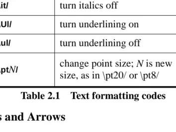
2.1 Text formatting codes . . . 32

3.1 Characters used to define columns . . . 56

3.2 Default column definitions . . . 57

3.3 Math functions . . . 61

3.4 Mathematical operators . . . 62

6.1 Equation Constants and Macros. . . 93

(13)

(14)

xi

Preface

EasyPlot is a tool for viewing, analyzing, and plotting scientific data. It is designed for anyone who works with scientific or engineering data. EasyPlot provides a powerful graphical environment in which you interact directly with graphs and data.

The philosophy behind EasyPlot is to make what most people do most of the time as simple as possible. You should find EasyPlot’s menu system compact and straightforward. You will not find layers of complicated dialog boxes; EasyPlot has a few neatly laid-out dialogs that control key aspects of graphs. Details of fine-tuning EasyPlot and your graphs are organized in aPreferences dialog that gives you access to loads of special features.

If you are not familiar with EasyPlot, don’t be fooled by its small size and uncluttered appearance. The entire program is one executable file that occupies around 700K of disk space. A great deal of engineering has gone into keeping EasyPlot small and the result is a program that does a lot, runs quickly, and takes up relatively little disk space.

The original EasyPlot was developed over a two and a half year span (1986– 1989) at MIT Lincoln Laboratory. Lincoln Laboratory provided an ideal environment for developing a general-purpose plotting program; I was surrounded by scientists who used the software, provided endless constructive feedback, and could get updates whenever I implemented a new feature. Today, the Internet is extending Spiral Software’s corridors around the world and, once again, scientists and engineers (that’s you) can participate in EasyPlot’s development by submitting ideas and receiving software updates minutes after a new feature is implemented. I urge more of you to communicate even the smallest suggestions; your ideas fuel EasyPlot’s growth and development.

Stuart Karon [email protected]

(15)

(16)

1

Chapter 1:

Getting Started

1

1.1 System Requirements

EasyPlot for Windows will run on any PC system running Windows 95, Windows 98, 2000, ME, XP and Windows NT.

1.2 Installing and Running EasyPlot for Windows

Place the EasyPlot diskette into your computer and runsetup.exe.

EasyPlot for Windows consists of one file, epw.exe for 16-bit EasyPlot, or

epw32.exe for the 32-bit version. EasyPlot also comes with a supporting help file (help.ep) and a few small data files. EasyPlot does not add or modify any files in your Windows directory. If you need to remove EasyPlot from your hard drive, simply delete the files in the EasyPlot directory and remove the EasyPlot icon from your Windows desktop. Or use theUninstall utility loaded with EasyPlot.

When you run EasyPlot, an empty graph appears and EasyPlot prompts you for something to plot (an ASCII or binary data file, a spreadsheet file, an equation,...). Answer the prompt and a graph appears. To overlay more curves on the same graph, clickFile /Open and load another data file. ChooseFile /New to create a new, empty graph.

EasyPlot has two menus (§7.8). One is more compatible with earlier versions of EasyPlot; the other is more Windows standard. The Windows-standard menu is selected when you first install EasyPlot. If you are familiar with old versions of EasyPlot, or plan to use EasyPlot’s batch language to automate graphing, you may prefer the EasyPlot-standard menu. To switch, pull downFile, runPreferences,

(17)

and go to theUser interface topic. The two menus are very similar and you can switch from one to the other at any time.

1.3 Selecting Curves

Much of what you do with EasyPlot centers around curves on graphs. There are several ways to select curves on graphs with many data sets displayed. If you run a function that operates on a curve (such asTools /Curve fit), you need to select a curve, assuming there is more than one curve on the graph. You can select a curve before you choose the operation, or after. If no curve is selected when you run a curve function, EasyPlot displays a list of curves and prompts you to select one.

If you select a curve before choosing the curve function, you can do it right on the graph. Click on a curve to select it. A piece of the curve appears on the help line at the bottom of the EasyPlot window (the staus bar) to show you which curve is selected. If a curve is already selected and you click near the selected curve but want to pick another nearby curve, you may notice a small delay before the next curve shows up as selected; the delay gives you time to double-click before EasyPlot changes the selected curve.

You can also select curves with the<space> bar or the right mouse button. If you use the right mouse button, be sure to click on an empty part of the graph; otherwise, you’ll activate a context-sensitive right-mouse menu. Each time you press the right mouse button or<space> bar, EasyPlot selects the next curve on the graph. When you reach the last curve, EasyPlot cycles back to the beginning. If you hold the<space> bar or right mouse button, the selected curve glimmers, making it easy to spot on a crowded graph.

1.4 A Guided Tour

This section guides you through creating a graph and using a few of EasyPlot’s special features. We’ll begin by reading a couple data files and looking at the data with EasyPlot’s visual-analysis tools. We’ll do some mathematical analysis on the data, title and annotate the graph, and then take a look at the final results.

The tour covers commonly used features and should help you get started using the program. It is not a comprehensive introduction to EasyPlot; the topics discussed represent only a fraction of EasyPlot’s capabilities. Throughout the introduction, notice that you always work directly with graphs, not columns of numbers.

(18)

1.4. A Guided Tour 3

1.4.1 Loading Data

To begin, we’ll load a few data sets. Run EasyPlot and, at theOpen dialog, select

Data2 in the EasyPlot directory. Click the Open icon ( ) on the help line (the status bar), or click File / Open, and load Data3. Data2 and Data3 are short, ASCII data files provided with the program.

1.4.2 Data Viewing Tools

Zooming in Click and drag the cursor to define a zoom rectangle on the graph.

When you release, EasyPlot expands the data inside the zoom rectangle (§2.15).

Zoom in a few more times. There’s no limit to the number of times you can zoom .

Scrolling Once you’ve zoomed in, you can use scroll bars (§2.16) to shift your

view of the data. Pull downTools and selectScroll. Try scrolling. If you do a lot of scrolling, turn on<Scroll Lock> to use cursor arrow keys to scroll the graph.

Zooming Out There are several ways to zoom back out. To return to the

previous zoom level, hold<Ctrl> and click on the graph. EasyPlot remembers up to five zoom ranges. To zoom all the way out, Autorange the graph. Click the

Autorange icon ( ) on the help line, orOptions /Autorange. TheAutorange

feature (§2.17) sets axis ranges to include all data and major tics at the axis ends.

Reading Coordinates from the Graph Turn scroll bars off and select Tools /

X-hair. Move the cursor inside the graph. EasyPlot displays the x- and y-coordinates of the cursor in two small windows above the graph (§4.14). You can lock the cursor to a curve by clicking on the curve you want to track. Hit

<esc> or move the cursor off the graph to unlock from the curve. You can disable the lock-to-curve feature by right clicking on one of the cross-hair windows. Turn off theX-hair tool; clickTools /X-hair, or right click on a cross-hair window.

(19)

1.4.3 Mathematical Analysis

EasyPlot’s mathematical analysis tools compute curves and statistics based on existing curves. EasyPlot gives you the option to save the computed data to a separate file. If you don’t care about saving computed data to separate files (it is saved with the graph otherwise), you can turn off the save prompt. For the analysis steps below, we assume the save computed data option is off. Click

File/Preferences, scroll to the Safeties topic, and make sure that the option

Prompt to save computed data is off.

Curve Fitting Pull down theTools menu and selectCurve fit. Choose to fit the

Data2 curve, the one with open-circle markers. If you select a curve before runningCurve fit (by clicking it on the graph), EasyPlot would not prompt you to select a curve. At the Curve fit dialog (§4.5), enter “2” and hit OK. The fitted curve appears on the graph and EasyPlot puts the fit equation above the graph. The equation is an annotation that you can move, edit, or delete. Because curve-fits can shoot way off the graph, EasyPlot locks the axis ranges (turns autoranging off) before plotting fits. Later on, we’ll need to autorange an axis as a result of having fit a curve.

Statistics Click on theData2 curve; a piece of the curve appears on the help line (or “status bar”) to show it’s selected. Pull down Tools, go to Stats, and run

Mean, Std Dev,... (§4.6). Notice you’re not prompted to select a curve. EasyPlot places the statistics on the graph as an annotation which, like the curve-fit equation, you can move, edit, or delete. Click on the note and drag it to the middle of the graph:

Smoothing Click on theData3 curve and runTools /Smooth. You can smooth

data (§4.10) with a sliding average or by averaging all the points within range segments on the x-axis. Choose the sliding data window and select a 5-point window. The smoothed curve appears on the graph.

(20)

Transforming Data In spreadsheets, you can compute new columns of data

from mathematical operations on existing columns. In EasyPlot, you can create new curves by applying equations to existing curves (§4.2). Click on the Data3

curve again and runTools /Transform. There are three options in the bottom-left corner of theTransform dialog. Make sureKeep original curve is checked and entery = 7log(y). Multiplication is implicit; you do not need to type7*log(y). The transformed curve appears near the bottom of the graph.

1.4.4 Customizing Axes

The new curve (the log ofData3) does not show up well on the y-axis that runs from 0 to 150. Let’s plot the transformed curve on its own y-axis and then adjust the range and tic positions on an axis.

Private Axes Any curve on anxy graph can have its own “private” x- and/or

y-axis (§2.14). Private axes are color-coded to the curve and while they are called “private”, you can plot any curve against another curve’s private axes. Right click on the transformed curve, select Private axes..., and click Y-axis. A new axis appears to the left of the primaryy-axis.

Range & Tic Positions So far, EasyPlot has set the range and tic positions for all the axes. Double click on the private axis. At the top of theAxis Setup dialog (Figure 2.13), enter14 inCoor of a major tic,0.2 for theMaj tic increment, and

1 for # of minor tics. Click OK. Note that the range changes to 14.2 to 15.2; autoranged axes include all data and major tics at the axis ends and when you change tic positions on an autoranged axis, the range can change, too.

Axis Markers Click from oney-axis to the other. EasyPlot draws a small

color-coded marker for each curve plotted on the selected axis. Now click from one curve to another. A single color-coded marker appears above the axis on which the curve is plotted. The markers show you how curves and axes are organized and can be very helpful on complicated graphs.

Floating Tic Marks You can add individual “floating” tic marks anywhere on

an axis to highlight special values (§2.11.4). Double click on the private y-axis (the transformed curve’s y-axis) and selectFloating tics... in the top right of the

Axis Setup dialog. Add a tic at 14.86, and enter “median” in label for tic. (14.86 is not the true median but it’s close.) Click OK to close both dialogs. You can label entire axes with floating tics to read day-of-week or month, for example. Or use them to produce custom, nonlinear scales, such as for probability plots.

(21)

Secondary Axes In addition to primary and private axes, you can put a second x- and/or y-axis on graphs (§2.14). Secondary axes appear on the right and top sides of the graph. Right click on the primaryy-axis and selectAdd 2nd Y-axis. The new axis inherits the range and tic positions of the primary axis. The open marker above the new axis tells you that no curves are plotted against it. Let’s move the two top curves ( ) to the right-hand axis. Right click on one of them and chooseSelect axis... EasyPlot shows you a piece of the selected curve on the help line along with the prompt “Click on axis to use...”. Click on the right axis. The only change you should see is in the marker above the axis. If the secondary axis were set to autorange, it would have rescaled automatically upon having a curve assigned to it. But it inherited the range of the primary axis and because of the curve fit we ran earlier, the primary axis was not autoranged. Double click on the right-handy-axis and set theAutorange checkbox. HitOK. Right click on the other top curve and useSelect axis... to move it to the secondaryy-axis. Notice that two of the curves (Data3 and its log) almost overlap but click on them and watch the axis markers; you’ll see that they are plotted on different scales and based on the axis ranges, they are quite different.

1.4.5 Annotating and Titling Graphs

Assuming we have all our data on the graph and are finished analyzing it, it’s time to make the graph presentable to others. We start by creating a legend.

Legend Click Options /Legend. A legend box appears on the graph (§2.12).

Depending on your Legend Preferences, the box should have one, three, or no entries. Right click on the legend and select Legend Preferences. The bottom two checkboxes tell EasyPlot whether or not to assign default legend titles to curves generated from equations or loaded from files. When you first install EasyPlot,Put eqn in legend is checked butUse file & column #is not. EasyPlot assigns default legends only when a curve is created; changing the legend preferences will not add or remove legend entries for existing curves. Turn on the two bottomLegend Preference checkboxes and clickOK.

Detour — Saving a graph If Data2 and Data3 do not appear in the legend,

here’s a trick to get EasyPlot to assign default legend titles (now that we’ve turned the options on). ClickFile / Save and, in theSave dialog, make surePut data in file is not checked. Save the graph. WithPut data in file off, the save file contains links to the data files you loaded, in this caseData2 andData3. Other curves that

(22)

do not correspond to data files will be stored right in the save file. Save the graph and then open the save file (File / Open or File /New). Now Data2 and Data3

should appear in the legend.

To add or edit legend titles, right- or double-click on a curve and chooseLegend. If the curve already appears in the legend, you can double click on its legend title. Right click on the transform curve, selectLegend, and enter “Log of data3” .

Rearranging Legend Entries Let’s move Data2 and Data3 to the top of the

legend. Click Window / Curve toolbar. On the right of the Curve Toolbar is a 3-part legend button. The arrows move a curve up or down in the legend. Click on

Data2, on the graph or in the legend, and then click the up arrow untilData2 is at the top of the legend. SelectData3 and move it up and belowData2.

Annotations The statistics information we computed earlier on Data2 was

placed on the screen as an annotation.<Alt> click on the note and remove all but the first two lines. Click off the note or hit<Ctrl><Enter> when finished. If the text overlaps other graph objects, drag the note to an empty spot on the graph. Right click on the note, selectProperties..., and set the color of the note to blue to match theData2 curve. The equation above the graph is also an annotation. Click and drag it into the top of the graph.

You can add any number of annotations to a graph (§2.7). Create a few new ones by clicking the annotation icon ( ) on the help line, Add / Annotation, or by

<Alt>clicking on an empty spot on the graph. When finished typing, hit<Enter>

twice at the end of a note; or hit<Ctrl><Enter> if the text cursor is not at the end of the note; or just click off the note.

Lines and Arrows You can sketch lines and arrows on the graph, to point from

a note to the curve it describes, for example. Click the line-draw icon ( ) on the help line, orAdd /Line (§2.9). The cursor turns into a pencil. Hold the left mouse button and move the cursor to draw a line. Hold<Alt> when pressing or releasing the mouse button to put an arrow head on the line. Draw a line on the screen from the statistics note to the Data2 curve. Draw another line from the equation to the fit curve. Hit <Esc> to leave line-draw mode. Right click on the first line, select

Properties..., and make the line blue. Repeat for the second line to match its color to the fit curve and the equation.

Titling the Graph and Axes The open boxes around the graph let you enter

(23)

1.4.6 Previewing and Printing

When finished laying out the graph, you can see what it will look like when printed. Pull down File and run Print Preview (§8.2). You can zoom in on the preview the same way you zoom in on data in “working” mode. In the previewer, however, you zoom the entire view rather than just the graph range. Zooming out also works the same; use theAutorange feature or right click on the preview and selectFit to window.

You can move objects on the graph and even edit titles and notes. Editing in the previewer is a little slower than in “working” mode; if performance is important to you, use the previewer for final touch-up work only. When ready to print, click

Print... in the main menu; or right click and select Print... or Print now. The

Print... buttons open thePrint dialog and let you modify settings before printing. ThePrint now button and the print icon on the help line send the graph directly to the currently selected printer.

1.4.7 Multiple Graphs on a Page

Pull down File and choose Close all. EasyPlot creates a new, blank graph and asks for something to plot. ClickGraph a function... Make sure theTrig mode is set toDegrees and enter “sin(x)”. Because there is no data on the graph and thus no definedx-range, EasyPlot prompts you for a range over which to compute the equation. Enter “0 1440”. Click File /New and, again, chooseGraph a function...

Before entering the function, click on the button labeled 150 Points... (150 is EasyPlot’s default; your Points button may show a different number.) For this curve, we should compute more than 150 points. Enter 600. For the equation, type “sin(x) + .2sin(10x)” and use the same x-range, 0 to 1440.

If you plot a lot of functions and use EasyPlot’s more Windows-standard menu (§7.8), useAdd /Function instead of File /Open. Or, use the EasyPlot-standard

Open dialog which switches automatically between file and equation modes based on what you type. You choose which menu andOpen dialog to use in the

User Interface topic of thePreferences dialog (File /Preferences).

We now have two graphs, one on top of the other. Hit<Ctrl><Tab> to cycle from one to the other. Pull down theWindow menu and you’ll see the two graphs at the bottom of the menu with a check mark next to the top graph. Select Tile and choose a 1x2 layout. The bottom of theTile dialog shows you the graph layout. You can use theGap setting to add extra space between graphs or to bring graphs

(24)

closer together but for our purposes, leave theGap at 0. ClickOK and you should see both graphs.

You can link axes together so that a change in one is reflected in all linked axes. EasyPlot’s “Axis Linking & Mirroring” feature (§2.14) is a handy tool for keeping bothx- andy-axes identical. Right click on anx-axis and selectMirror axis... The cursor turns into a small cross-hair and, on the help line, EasyPlot prompts you to click on another axis. Click on the other x-axis. A small mirror marker appears below each axis near x_max. The two axes are now linked but since they were already identical, neither graph changes.

Right click on the y-axis of the first graph (the one with the smooth sine curve) and mirror it to they-axis on the other graph. This time, the first graph changes to take on they-range of the other graph.

Double click on anx-axis and enter “1500” for the axis maximum. Click OK and both graphs display the new range. Double click on anx-axis and enter “180” for the distance between major tics (Maj tic increment). Again, the change is reflected on both graphs.

Double click on anx-axis. Turn onLet EasyPlot Place tic marks and clickOK. Zoom in on one of the graphs. With the x- and y-axes linked, zooming on one graph also zooms the other.

To break the link between axes, right click on an axis and chooseBreak mirror. That concludes our tutorial. You should now be ready to use EasyPlot to create your own graphs. If you have questions that aren’t answered by the manual or on-line help, feel free to contact Spiral Software or Cherwell Scientific by phone or e-mail. Enjoy the software!

(25)

(26)

2.1. Plotting Data 11

Chapter 2:

Making Graphs

2 2

2.1 Plotting Data

To plot a data file (ASCII, binary, or spreadsheet), an equation, or to enter data, pull down File and selectNew orOpen; or click on theNew( ) orOpen( ) help-line icons. New creates a new graph on top of existing graphs;Open adds data to a graph. EasyPlot displays one of twoOpen dialogs:

Under Windows NT or 95, EasyPlot uses the Explorer-style Open dialog by default. Under Windows 3.1, EasyPlot uses the dialog on the left. The W3.1Open

dialog automatically switches to equation mode if you start typing a function. To plot a function with the Explorer-style dialog, click on the Graph a function...

button. If you run NT or 95 and prefer the Open dialog that switches automati-cally between file- and equation-mode, go to the User Interface topic of the

Preferences dialog, and select to use the EasyPlot-standardOpen dialog.

From theOpen dialog, you can read ASCII and binary data files, spreadsheet files (.wk1,.xls, or.wq1), an EasyPlot save file, or you can generate curves with equations. If you enter the name of a file that does not have one of the spreadsheet

(27)

extensions listed above, EasyPlot assumes it contains ASCII data and/or EasyPlot batch commands. (EasyPlot save files are ASCII files containing EasyPlot batch commands and possibly data.)

To read a binary data file, use theOpen as dropdown to select the file format: 1-, 2-, or 4-byte integer, 1-, 2-, or 4-byte unsigned integer, and 4- or 8-byte float. After choosing a format, EasyPlot displays a list of file-reading options that lets you specify the number of data columns, the number of header bytes to skip before reading data, etc. See Section 2.1.5 for details on reading binary files.

By using theOpen button repeatedly, you can overlay any number of data sets on a graph. To keep data sets distinct, EasyPlot supports seven dash patterns and fourteen data marks. You can also differentiate data by displaying them with different styles – one as a scatter plot and another as a line plot, for example. Section 2.2 discusses how to customize the appearance of your data.

2.1.1 Listing Specific Files Types

By default, the Open dialog lists all files types. You can modify the default file types listed by entering custom file specifications in the User Interface topic of the Preferences dialog. You can enter several file specifications separated by a space or comma, for instance “*.dat, *.ezp”.

2.1.2 Browsing Files

To view and/or modify data before plotting, turn on theBrowse file checkbox in the Open dialog. EasyPlot loads the file you select into its built-in Data Table. Once in the Data Table, click on Plot or hit <alt>P to plot the file. See Section 7.9.2 for more details on editing files. The Data Table lets you browse and edit ASCII and spreadsheet files; it does not load binary files. To load binary data, plot it and thenEdit theData.

2.1.3 Entering Data

To type data directly into EasyPlot, click on Enter data in the Open dialog or chooseFile/Enter data. You enter data into EasyPlot’s Data Table (§7.9.2). Move from cell to cell with the cursor-arrow keys or the mouse. After entering a number, hit<space> or<tab> to move to the next column. Hit<enter> to move down a row and back to the first column.

EasyPlot assumes the first data column is x and subsequent columns y (§3.4). Click on the definition at the top of a column to change its definition. Click on

(28)

Plot or hit<alt>P to plot what you’ve entered. If Close after plot (under the Data Table File menu) is not checked, the table stays open after plotting data and you can continue entering or editing data. If the table closes, you can load data back into the table by pulling down EasyPlot’s Edit menu and selecting Data. See Section 3.1 for details on how to format data files.

2.1.4 Plotting Data in the Clipboard

If you have copied data to the Clipboard in another application, you do not need to import the data into EasyPlot’s Data Table before plotting. Simply Paste the data onto the graph (^V or Edit/Paste) and EasyPlot automatically converts the text data on the Clipboard to curves.

2.1.5 Reading Binary Data Files

To read binary data, click onOpen as in theOpen dialog and select the binary format that matches your data: 1, 2, 4, or 8-byte integer (signed or unsigned), or 4 or 8-byte floating point. EasyPlot then displays a file configuration menu:

If a file has header information, use theheader bytes button to tell EasyPlot how many bytes to skip before reading data. You can also use the header to skip over a section of data at the top of the file. If a file has 1000 pairs of 2-byte integers, for example, and you want to plot only the second half of the file, you can set the header to 2000 bytes (500 pairs * 4 bytes/pair).

Thedata columns specifies how many columns of data the file contains. A file with alternating x and y values, for example, has 2 columns. If the number of data columns is 0 (as it is by default), EasyPlot will not read any data from the file. The next two options, the skip values, let you read every nth data row or only one or two columns out of a multiple-column file. The first skip value tells EasyPlot how many bytes to skip after reading a data point. The second specifies how many bytes to skip after reading a data row. To read every 10th row of a 6-column, 2-byte-integer file, for example, selectskip M bytes between rows and enter 108 (12bytes/row * 9 rows). If you want only the 2nd and 4th columns of the

(29)

file, add 2 bytes to the header (to skip the first data point), skip 2 bytes between columns (to step over columns 3 and 5), and add 4 to the between-row skip (to step over column 6 and the first column of the next row).

The last option lets you average every M rows to produce an average row, thereby reducing the number of data points without losing magnitude information. Averaging every 10 points, for example, turns a 100,000-point file into a 10,000-point file. If you set the between-row skip, EasyPlot averages only the rows that are read, not those that are skipped.

When finished setting the file-reading options, click outside the popup menu. If you need to go back to the options list, click on theOptions... button.

2.1.6 ASCII File-Reading Options

When reading ASCII files, you can have EasyPlot start and stop reading the file at specific lines, read every Nth data row, and average every N data rows to produce

M/N average rows, where M is the total number of rows read.

With the Open dialog set for reading ASCII files (in Open as), click

Options... and EasyPlot displays the following options:

Thebegin andend options let you tell EasyPlot where in the file to begin looking for data and at which line to stop reading the file altogether. When skipping lines at the beginning of a file, EasyPlot ignores all data but will process batch commands. Once it reaches the “end” line (if one is set), EasyPlot stops reading the file and will not process any subsequent data or batch commands.

Theread every Nth row option lets you take every Nth data row of a file. The

average every M rows lets you reduce the number of data points by averaging every M rows together to produce one average row. The average feature takes into account only those rows which are read; if you read every Nth row, EasyPlot aver-ages every Nth row until it gets M rows averaged.

The ignore text option tells EasyPlot to ignore all text that is not part of a batch command. By default, EasyPlot jumps ahead to the next line after finding any non-numeric character. With ignore text on, EasyPlot skips over text and continues scanning the line for data.

(30)

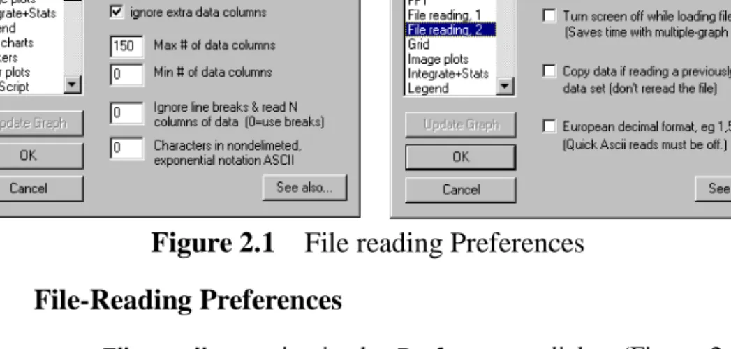
2.1.7 File-Reading Preferences

There are two File reading topics in the Preferences dialog (Figure 2.1) that provide several options for customizing the way EasyPlot reads files.

Put filename on graph: You can put the name of each file on the graph by turning onShow filename. The name appears as an annotation at the coordinates specified below the Show checkbox. If you read several files, the names appear on top of one another unless you move them. You can move, edit and delete the filenames as you would any annotation.

Read quoted data: By default, EasyPlot does not read quoted numbers as data. If files have columns of quoted data, turn onRead quoted data.

“;” ignores rest of line: With ASCII files, EasyPlot ignores the remainder of a line upon finding a non-numeric character. If you turn “ignore text” on (§2.1.6), the only way to comment out portions of a file is to turn on “;” ignores rest of line and put semicolons in front of lines you want to ignore.

Ignore extra data columns: EasyPlot determines the number of columns in ASCII files by counting how many numbers are on the first data row. If it finds N numbers, it ignores rows that do not have exactly N numbers. If some of the rows have extra values after the N columns, you can ignore the extra columns rather than the entire row by turning onignore extra data columns.

Max # of data columns: By default, EasyPlot reads up to 150 data columns. If you read files with more than 150 columns, increase the number in theMax # of

(31)

data columns edit box. The absolute maximum is 1024. Larger values require more memory for reading files.

Min # of data columns:When reading ASCII data files, EasyPlot determines the number of columns by the first row of data it finds. If the first data row is missing one or more values and you don’t want to modify the files to insert missing value place-holders (//m -- §6.3), you can tell EasyPlot the minimum number of data columns to accept. EasyPlot will ignore data until it finds the first row with at least the specified minimum number of columns.

Ignore line breaks: Rows of ASCII data are usually delimited by line breaks. Otherwise, you can tell EasyPlot how many columns of data to read and it will ignore line breaks altogether. With XY pairs strung over a single line, for example, enter 2 in theIgnore line breaks edit box. EasyPlot scans for two data points, installs them as a data row, looks for the next two points, and so on. You need to enter 0 to go back to using line breaks. The batch command for turning this feature on is “//columns N”, where N is the number of columns. After reading the data, you should resetIgnore line breaks back to zero.

Fixed exponential notation: If a file contains data in fixed-length exponential notation, some values may not have a space or other character separating them from their neighbors. To read such a file, enter the length of the data values in the

fixed exponential notation edit box.

Allow Quick ASCII reads: If you read large ASCII data files, EasyPlot will load them much quicker with this option on. Files can contain header comments and EasyPlot batch files but only before the data. The quick ASCII read does not support missing values or some other file-reading options, such as European decimal format. If you are having trouble loading data andQuick ASCII read is on, try turning it off. The quick ASCII read can save a significant amount of time with very large data files (tens of thousands of points). With smaller files, the difference can be insignificant and we recommend you leave this option off.

Assume only integer data: TheQuick ASCII read can load data about twice as fast if the values are all integers. If values do have fractional components and this option is set, the data will not load correctly.

Turn screen off while loading files: EasyPlot draws graphs as it reads files so that you see the graphs you’re loading. If your save files contain many graphs, you can save time by not updating the screen until EasyPlot finishes reading the file.

Copy data if reading a previously loaded data set: When plotting different columns of the same data set on separate graphs, EasyPlot does not let you share

(32)

2.2. Styling the Data 17

data from one graph to the next. Rereading can be time consuming but you can save time by allowing EasyPlot to make a copy of the data it has already loaded instead of rereading the file. If the file contains EasyPlot batch commands, they will not be executed for the copied data.

European decimal format: Normally, EasyPlot treats commas as column delim-iters. The European decimal format option tells EasyPlot to assume commas separate the integer from the decimal part of a number. With this option off, Easy-Plot reads “2,4” as two values, “2” and “4”. With it on, it reads “2,4” as “2.4” .

2.2 Styling the Data

You can display data in a variety of formats, such as scatter, line, or bar. EasyPlot provides a list of style attributes which you can turn on or off for the entire graph or for individual curves. Pull down theStyle menu and you see the style options:

New curves inherit the styles that are on at the time. Switching styles on and off does not affect data on the screen. To change the appearance of data, use the

Restyle button (underStyle) or double click on the data and turn style attributes on or off in theData Style dialog (Figure 2.2 – §2.4).

(33)

EasyPlot starts withConnect Pts,Mark Pts, andDash as defaults styles. You can use EasyPlot batch commands to change the defaults (§6.4) or to toggle styles on and off from within a data file (§6.1).

2.2.1 Selecting the Data Mark, Color, Dash, & Fill

EasyPlot assigns an attribute set to each curve which determines the curve’s color, data mark, dash pattern, and bar fill pattern. To change the attribute set of a curve, double-click on the curve and select mark,dash & color... in the Data Style

dialog. EasyPlot lets you pick one of the 14 predefined attribute sets or create a custom set. Curves can share the same attribute set.

EasyPlot supports 14 geometric data markers, 14 bar fill patterns, 7 curve colors, and 7 dash patterns. Attribute sets 1-7 share the same colors and dash patterns as sets 8-14 but have unique data marks and bar fill patterns.

In addition to the geometric markers, you can mark data with any ASCII char-acter or its data values. Click on mark,dash & color... and choose the custom

option. EasyPlot prompts you to select a marker (assuming markers are on). To use a character, pickletter and enter the letter. To use data values, pickX-coor or

Y-coor. If the data has a column ofz-values, you can chooseZ-coor.

Another method for changing the attribute set of a curve is to hold the right mouse button (be sure the cursor is not on any graph object) or space bar so that the curve glimmers (§1.3) and hitc for “color”. EasyPlot assigns the next attribute set to the curve; if it had set 5, for example, it gets 6. Repeat until you find a set you like. At set 14, EasyPlot cycles back to 1.

You can specify an attribute set for a curve in a data file with the command:

/sa m n [c]

where n is a number from 1 to 14 and c is an optional column number. Place the command before the data it is to describe If you don’t specify the column number, EasyPlot assigns the attribute set to column 2.

2.2.2 Data Marks

EasyPlot can mark data with any of the 14 marks in Figure 2.4, any ASCII char-acter, or thex-,y-, orz-value of each point. Section 2.2.1 discusses how to select a particular data mark.

If a data set has many points, you can mark at every Nth point. Double click on a curve with markers and enter a number in theat every point edit

(34)

box. If you enter a 2, EasyPlot places a mark at every other point. If you enter 10, it marks every 10th point.

On contour maps, themark pts style creates a color map or image plot. Each data point is marked with a color or gray scale representing its height. You can select color or gray-scale images inImage plots Preferences.

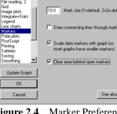
2.2.3 Marker Preferences

Mark size:Marker size affects all curves on all graphs. Enter 2 to double marker size, 0.5 to half their size, or 1 to use the default size. EasyPlot bases the default mark size on the size of the graph. If you use 0 as the mark size, EasyPlot places a dot at each data point. On screen, EasyPlot does not draw markers smaller than 3 pixels so that you can distinguish the mark shapes. When you print, they will be scaled exactly as you specify, down to a dot if the size you enter is small enough.

Figure 2.3 The 14 Data Marks

1 2 3 4 5 6 7 8 9 10 11 12 13 14

(35)

Draw connecting lines through markers: If a curve has connecting lines and markers, you can draw lines through markers or break them to not hit the marks:

Scale data marks with graph: With different sized graphs on the same page, you can have EasyPlot scale markers so that small, inset graphs have smaller markers than larger graphs. When not scaled, all graphs have the same size markers:

Clear area behind open markers: EasyPlot can draw open markers as truly open or fill them with the background color. When open markers overlap, clearing can make the graph look neater.

2.2.4 Connecting Lines

If a curve is drawn with connecting lines, EasyPlot draws a straight line from each point to the next. Connecting lines are drawn dashed if the dash style is on and solid ifdash is off. EasyPlot supports seven dash patterns (Figure 2.4). EasyPlot assigns a color and dash pattern to each curve. Section 2.2.1 discusses how to select the color and dash pattern used for a curve.

On curves with connecting lines and data markers, you can pass the lines through the data marks or break them so they do not hit the markers (§2.2.3).

Draw through Miss marks Scale marks Don’t scale Clear Leave open

Figure 2.5 The 7 Dash Patterns

1 2 3 4 5 6 7

(36)

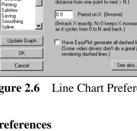
2.2.5 Line chart Preferences

ThePreferences dialog (underFile) has aLine charts topic that lets you set the default line weight for connecting lines. You can also choose to break curves at missing data points (otherwise EasyPlot connects the last non-missing point to the next non-missing point).

Break curves at missing points: If a curve has missing values (§6.3), EasyPlot can break the curve at missing values or keep the connecting lines contiguous by ignoring missing points.

Default line weight: Normally, EasyPlot assigns a line weight of 1 to curves, meaning that the curves are drawn with the same line weight as the axes and tic marks. You can increase the line weight for individual curves by double clicking on the curve. If you want all curves to get a heavier line weight by default, enter the desired number in theDefault line weight edit box.

Longest connecting line: This option lets you highlight discontinuities in data. Enter the longest line you want EasyPlot to draw and if two points are further apart than the specified length, a break appears in the curve. Specify the distance in graph coordinates. Enter ‘0’ to connect all points .

Period on X: If data is periodic on X, for instance 0,1, 2,... 360,0, 1, 2,..., the curve will trace back and forth across the graph. If you want the X-values to appear as though they are sequential in time, enter a period value for X. EasyPlot

(37)

adds the value to a base X-coordinate each time the data cycles backwards.

Have EasyPlot generate all dashed lines: Maintaining a consistent dash pattern along curves consisting of many short line segments is a tricky procedure. EasyPlot generates all dashed curves when printing, but on screen, it lets the Windows video driver do the drawing (assuming it’s a single-pixel width line; Windows doesn’t support multiple-pixel-width dashed lines). Many video drivers do not do a very good job rendering complicated dashed lines. If you see strange-looking dash patterns, turn on this option and EasyPlot will draw all dashed lines.

2.2.6 Error Bars

For any curve on an xy plot, EasyPlot can draw x-error bars, y-error bars, or both. To create error bars, you must place error values in the data file along with the x-and y-values x-and you must tell EasyPlot which column or columns are error values. You can then turn x- and/or y-error bars on and read in or restyle a data set. Error Values in Data Files

In the data file, error values occupy columns. With one error column, you can draw either x- or y-error bars. With two error columns, you can draw x- and y-error bars or asymmetric error bars. Forx- andy-error bars, the first, or left-most error column maps to the independent axis (usually x) and the second maps to the dependent axis. For asymmetric error bars, the first error column represents the ‘up’ error and the second column the ‘down’ .

TheError bars topic in thePreferences dialog controls how EasyPlot inter-prets error values. The upper two radio buttons determine whether error values specify the actual size of error bars or whether they are fractional percentages, and thus are multiplied by the x- or y-values to obtain the size of the error bars. The bottom two radio buttons tell EasyPlot whether with one error column, error values specify the entire up-and-down size of error bars, or whether they specify only half the total bar size (just the up or down height).

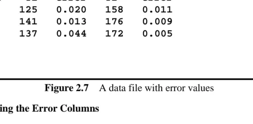
Normally, each y-column has its own column of error values and you would arrange the columns asXYEYEYE.... You can apply one error column to severaly -columns by placing the error between thex- and firsty-column, as inXEYYY. An example data file which includes error information is listed in Figure 2.7.

Without

period Period = 360

0 360 720 1080 0 90 180 270 360

(38)

Defining the Error Columns

You need to tell EasyPlot which columns of a data file are error values. Otherwise, EasyPlot assumes they arey-values and plots curves with them. Read in a data file that includes error information. Pull downTools and selectDefine Data. EasyPlot lets you edit the “column definition string” associated with the data file. This string has one character for each column of data; the first character in the string defines the first column of data, the second character defines the second column, and so on. To define error columns, place an e in the string positions that corre-spond to error values. Thee stands for “error”. For the example in Figure 2.7, the definition string is set to xyeye to define the first column as x, the second and fourth as y, and the third and fifth as error values. See Section 3.4 for more details on defining columns.

You can also define columns in the Data Table. In the Open dialog, turn on

browse file and load the data file. Or, plot the file and selectEdit/Data to load it into the Data Table. At the top of each data column, you see its definition in a small box. Click on the box to change the definition or double click to ignore the column. SelectPlot to apply changes to the graph.

If you generate your data files, you can define the columns by placing a batch command (§3.4) in the file, as illustrated in line 3 of Figure 2.7. That way, the columns will be defined properly every time you read the file into EasyPlot.

When EasyPlot first reads a file, it computes the data range for each column. If error values are predefined, EasyPlot takes the error into account in setting data ranges. Then, if you plot error bars, the autorange feature assures that data and the

This file results in two curves,

each with a column for making error bars.

/td xyeye ;define the columns

X Y1 error Y2 error 10 125 0.020 158 0.011 20 141 0.013 176 0.009 30 137 0.044 172 0.005 . . .

(39)

error bars fit in the graph. If you define error columns after plotting, you may have to stretch the range yourself to keep error bars from extending outside the graph. Turning On Error Bars

If you’ve read in data and defined error columns before turning the Error bar style on, double-click on the curve and turn on error bars in the Data Style dialog. Otherwise, pull down Style, select Error Bars, and choose an axis. Read in the data. If the file contains a batch command to define the error columns (see Figure 2.7), you should see error bars on the graph. Otherwise, define error columns as described above and you should then see error bars.

2.2.7 Three D Style

TheThree D style feature allows you to view data in three dimensions. You can plot data as 3D fishnet surfaces or as xyz triplets as a 3D scatter plot. You rotate the data by clicking on axis rotation buttons that appear in 3D mode. EasyPlot’s 3D feature is very fast and interactive, making it a powerful tool for visualizing 3D data. See Chapter 5 for details on working with 3D graphs.

2.2.8 The Bar Style

If a curve is drawn with theBar style, EasyPlot draws a bar from each point to the

x-axis. EasyPlot assigns a default fill pattern to each curve but you can select any

of EasyPlot’s 14 fill patterns (§2.2.1).

(40)

2.3. Font and Font Size 25

The width of the bars depends on the number of data points, the number of curves using the bar style, and a “bar spacing” value which you can adjust. If the bar spacing is 0, EasyPlot draws bars as wide as it can without overlapping them. If more than one data set is drawn with bars, EasyPlot makes the bars narrower so that bars can be displayed side-by-side without overlapping. Bar width is calcu-lated as n / (s + n), where n is the number of data sets displayed with bars ands is the bar spacing. To set the bar spacing or customize the with of the bars, go to the

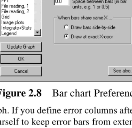
Bar charts topic of thePreferences dialog (Figure 2.8).

If you use a large value for theSpace between bars, bars become very thin. You can force EasyPlot to draw a line, or a needle, instead of a bar by using a value greater than or equal to 100.

If two data sets share the same x-values, you can display bars side-by-side or at their exact x-coordinates (and thus on top of each other). Use the two radio buttons labelledside-by-side orat exact X coor to choose.

If a data set has two x-values that are very close together, for example 1, 2, 2.01, 3,..., the bars will be very thin so that the 2 and 2.01 don’t overlap. You can force EasyPlot to draw wider bars by entering aWidth of bars value. Specify the width inx-axis units. Enter 0 to have EasyPlot compute the bar width.

You can adjust the darkness of the fill-patterns EasyPlot uses to distinguish bars of different data sets. For Bar fill density, enter a line-density scale value, where 1 is the default density, 2 doubles the line density, etc.

If you turn bars on for a polar plot, EasyPlot draws a line from each point to the center of the circle, producing what some people call a “wind rose” .

2.3 Font and Font Size

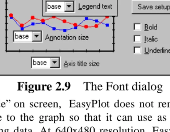
TheFont dialog (Figure 2.9) lets you select the font and text sizes used for graphs. The typeface you choose is used for all text on all graphs but you can make any text bold, italic, underlined, and any size independent of the rest of the text. To open theFont dialog, go toStyle /Font. You can also set point sizes in theFile /

Page Setup dialog.

There are five types of text you can put on graphs: tic-mark labels, axis titles, graph titles, annotations, and legend text. EasyPlot draws tic-mark labels at the base point size. You can set the size for each of the other types. You can override the defaults to make any text (or piece thereof) larger or smaller. Any annotation or part of a title, for instance, can be made larger or smaller than the default by using the point-size button in the Text Toolbar (§2.8).

(41)

In “working mode” on screen, EasyPlot does not render fonts in their true, physical size relative to the graph so that it can use as much of the screen as possible for displaying data. At 640x480 resolution, EasyPlot displays 12-point text with characters that are 12-pixels high, 20-point text with 20-pixel-high acters, and so on. With higher resolution screens, it scales the height so that char-acters appear about the same size as on a standard VGA screen. When you print or preview, text is scaled to its true point size.

EasyPlot can scale printed text based on the graph size so that small, inset graphs use smaller text than larger graphs. On a graph that takes up half the window, for example, 20-point text would print as 10-point text. You can turn text scaling on or off in Printing Preferences. You can also choose whether text is scaled relative to the largest graph on the page or relative to the full EasyPlot window. With two equal-sized graphs side-by-side, point text will print at 12-points if text scaling is off or scaled relative to the largest graph; otherwise text will appear smaller than the set size when printed.

2.4 Data Style Dialog

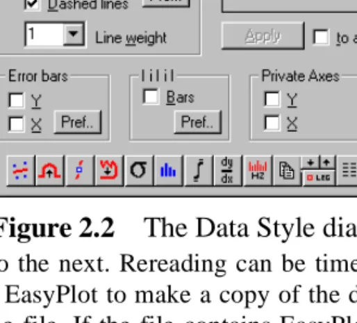
EasyPlot’s Data Style dialog (Figure 2.2) lets you set up a data set’s appearance. Double click on a curve, or right click and select Properties... If a graph has a legend, you can also double click on a data segment in the legend.

If markers are on, you can set marker frequency in theat every point

box (§2.2.2). If points are connected, you can set the weight, or thickness, of connecting lines in theline weight dropdown. You can use line-weight to

(42)

2.5. Polar Plots 27

entiate data sets. The mark,dash,& color... button (§2.2.1) lets you choose the

data marker, dash pattern, bar fill pattern, and the color used to display a curve. The Prefs... buttons jump you to Preferences topics for data markers, line charts, error bars, etc.

As you change styles, EasyPlot updates the curve-viewer button on the right side of the dialog. Click onApply to see the new styles reflected on the graph. If you update the graph and don’t like the new appearance, hit Cancel.

You can restyle all curves at once by turning on theto all checkbox next to the

Apply button. The curves will not look alike because they retain their individual mark, dash, and color attributes but they will all be drawn with the same styles.

You can switch from one curve to another without closing the Data Style

dialog. Click on the curve-viewer button (the one with a piece of the current curve displayed inside it) and select a curve from the popup menu. If you’ve made changes, EasyPlot applies them before switching curves.

You can enter or edit a curve’s legend title by clicking on the legend... button

(§2.12). Click onDelete to delete the selected curve.

TheData Style dialog has a toolbar along the bottom that lets you perform a variety of math and other operations on a curve. The buttons are identical to the Curve Toolbar (§4.5).

2.5 Polar Plots

For polar plots, enter data as radius and angle values and define the columns asr and t (t stands for theta, or angle). EasyPlot determines the graph type (xy or polar) by how the column are defined; if columns are defined with xs and ys, EasyPlot draws anxy plot. If rs andts, it creates a polar plot. Define columns in the Data Table or withDefine Data underTools (§3.4).

You can label angles around the plot by turning onLabel angles around plot

in thePolar plots topic of the Preferences dialog. The angular labels appear at intervals specified by the Angle between radial grid lines (also in Polar plots Preferences). Specify the angle in degrees. EasyPlot labels angles in degrees or radians depending on which trig mode is selected in theOpen dialog.

You can plot the entire circle, a semicircle, or a single quadrant. To set the angular range, you must be using the EasyPlot-standard menu (inUser Interface Preferences). Pull downEdit, chooseMove, and select x- ory-axis. See Section 2.11.6 for more details on setting angular range.

(43)

The angle origin (θ = 0) faces east by default. If you want the origin at the top of the circle or at any other location, go toPolar plots Preferences and enter the

Angle origin in degrees; 90 puts the origin due north, 180 west, or 270 south. The angle can increase clockwise or counter-clockwise (the default). Set the angle direction inPolar plots Preferences, with the Increase angle clockwise

checkbox. You can also plot only positive angles by setting the Plot absolute value of angles checkbox.

You can select data styles for polar plot data just as you would forxy curves. TheBar style on polar plots draws a line from each data point to the center of the circle, creating what in atmospheric studies is called a “wind rose” .

The x- and y-axes on polar plots are labeled identically. Turn major tics off (§2.11.3) for one axis to make the plot appear less cluttered. To change the radial range or location of tic marks, double click on thex-axis; they-axis mirrors thex.

2.6 Graph and Axis Titles

To place titles on graphs and axes, click on the small boxes above, to the left, and below the graph. After you click, the box disappears, the Text Toolbar (§2.8) pops up, and you can enter text. You enter graph and x-axis titles right on the graph. Because the y-axis title is rotated, EasyPlot opens a window for editing the y-axis title. When done, hit <enter> twice at the end of the text, ^<enter> with the cursor anywhere in the text, or click off the text. Once you’ve entered a title, click on it to edit. You can set the point size of titles independently from the rest of the text on a graph (§2.3). To title a second x-axis, add extra lines to the graph title.

2.7 Annotations

You can type annotations anywhere on a graph. Pull down Add and select

Annotation; or click the text icon ( ) on the help line. Or<alt>click where you want to put a note. When done entering text, hit<enter> twice with the cursor at the end of the text, ^<enter> with the cursor anywhere in the text, or click the mouse off the text. To leave a blank line, type a space before hitting<enter>.

If a note is not exactly where you want it, click and drag it to a new position. You can edit an existing note by double- or<alt>-clicking on it. To delete a note, right click on it and selectDelete from the popup menu. You can also click on the note and, while holding the left mouse button, hit<del> or<backspace>. If you click and release the mouse button without moving, the note remains selected and

(44)

2.7. Annotations 29

You can rotate annotations to any angle. Click on a note and, if you don’t move the note before releasing the mouse button, a selection box appears with arrows on each corner. Click and drag any corner to rotate the note. Hold<shift>

while rotating to move in 10 degree increments. To return a note to its default orientation, right click on it and selectClear rotation. Depending on the font you use and the font support in your version of Windows, rotated text may or may not appear in exactly the same typeface as unrotated text.

You can set the color and other details of how a note is displayed in the

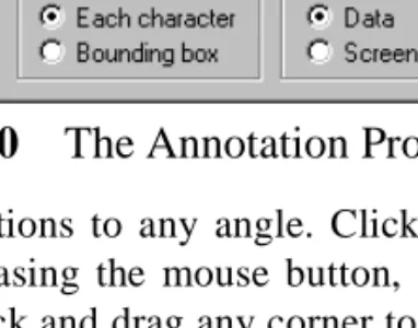
Annotation Properties dialog (Figure 2.10). Right click on a note and select

Properties... The dialog appears next to the annotation. You can set defaults for the properties inAnnotation Preferences.

You can draw a frame around a note. Turn the frame on or off in the

Annotation Properties dialog or by <ctrl> clicking on the note. You can also choose to clear behind the entire bounding box or behind individual characters.

You can place any number of annotations on a graph and each note can have up to 800 characters. Annotations and other text can include Greek characters, math symbols, superscripts, subscripts, and bold, italic, and underlined text (§2.8). Annotations placed inside a graph can be attached to a data coordinate or to a fixed screen location. (A note is considered inside or outside the graph based on the location of its first character.) Notes attached to data move with the data when axis ranges change. New annotations inherit the default specified inAnnotation Preferences. You can change the “attach” setting for existing notes in the

Annotation Properties dialog (Figure 2.10).

Figure 2.10 The Annotation Properties dialog

Frame &

Clear bounding box Clear behind individual characters

Easy Plot. Scientific Graphing and Data Analysis. Spiral Software. A product of

Easy

Plot

Scientific Graphing

and Data Analysis

Easy

Plot

For Microsoft Windows

Scientific Graphing and Data Analysis

by Stuart Karon

Spiral Software

The manual describes EasyPlot for Windows Version 4.0.

Copyright © 1988 - 200

2

by Spiral Software and Massachusetts Institute of

T

echnology

All rights reserved. No part of this manual may be reproduced, stored in a

retrieval system, or transmitted in any form or by any means, electronic,

mechanical, photocopying, recording, or otherwise, without the prior written

permission of MIT and Spiral Software.

Neither MIT nor Spiral Software make any guarantees as to the suitability or

accuracy of this program for individual applications.

Table of Contents

List of Figures

List of Tables

Preface

Chapter 1:

Getting Started

1

1

1.1

System Requirements

1.2

Installing and Running EasyPlot for Windows

1.3

Selecting Curves

1.4

A Guided Tour

Chapter 2:

Making Graphs

2.1

Plotting Data

2.2

Styling the Data

2.3

Font and Font Size

2.4

Data Style Dialog

2.5

Polar Plots

2.6

Graph and Axis Titles

2.7

Annotations