Ensemble Methods for Anomaly Detection

SURFACE

SURFACE

Dissertations - ALL SURFACE

December 2017

Ensemble Methods for Anomaly Detection

Ensemble Methods for Anomaly Detection

Syracuse University

Follow this and additional works at: https://surface.syr.edu/etd

Part of the Engineering Commons

Recommended Citation Recommended Citation

Zhao, Zhiruo, "Ensemble Methods for Anomaly Detection" (2017). Dissertations - ALL. 817.

https://surface.syr.edu/etd/817

This Dissertation is brought to you for free and open access by the SURFACE at SURFACE. It has been accepted for inclusion in Dissertations - ALL by an authorized administrator of SURFACE. For more information, please contact [email protected].

Anomaly detection has many applications in numerous areas such as intrusion detection, fraud detection, and medical diagnosis. Most current techniques are specialized for detect-ing one type of anomaly, and work well on specific domains and when the data satisfies specific assumptions. We address this problem, proposing ensemble anomaly detection techniques that perform well in many applications, with four major contributions: using bootstrapping to better detect anomalies on multiple subsamples, sequential application of diverse detection algorithms, a novel adaptive sampling and learning algorithm in which the anomalies are iteratively examined, and improving the random forest algorithms for detecting anomalies in streaming data.

We design and evaluate multiple ensemble strategies using score normalization, rank aggregation and majority voting, to combine the results from six well-known base algo-rithms. We propose a bootstrapping algorithm in which anomalies are evaluated from mul-tiple subsets of the data. Results show that our independent ensemble performs better than the base algorithms, and using bootstrapping achieves competitive quality and faster run-time compared with existing works.

We develop new sequential ensemble algorithms in which the second algorithm per-forms anomaly detection based on the first algorithm’s outputs; best results are obtained by combining algorithms that are substantially different. We propose a novel adaptive sam-pling algorithm which uses the score output of the base algorithm to determine the hard-to-detect examples, and iteratively resamples more points from such examples in a complete unsupervised context. On streaming datasets, we analyze the impact of parameters used in random trees, and propose new algorithms that work well with high-dimensional data, improving performance without increasing the number of trees or their heights. We show that further improvements can be obtained with an Evolutionary Algorithm.

By

Zhiruo Zhao

B.S. Northwestern Polytechnical University, 2011 M.S. Syracuse University, 2013

DISSERTATION

Submitted in partial fulfillment of the requirements for the degree of

Doctor of Philosophy in Computer and Information Science and Engineering (CISE)

Syracuse University December 2017

First of all, I would like to express my sincere gratitude to my advisors, Prof. Kis-han G. Mehrotra and Prof. Chilukuri K. MoKis-han, for the continuous support of my Ph.D study and related research. I thank them for encouraging my research and for guiding me to be a researcher throughout my Ph.D journey. I am also thankful for the excellent examples they have provided as successful researchers and scientists. I would also like to thank for my dissertation defense committee members: Prof. Vir Phoha, Prof. Qinru Qiu, Prof. Sucheta Soundarajan, and Prof. Ramesh Raina, for their time, interests and insightful comments.

My special thanks to Prof. Soundarajan and Prof. Reza Zafarani for giving me valuable feedbacks at our weekly research meeting. And all the professors at Syracuse University who have helped me throughout my graduate study.

I thank for all my lab mates and friends at our department, they are among the most brilliant people I have ever met. I would never forget all the discussions we have, all the fun projects we have worked on, and the support you gave me during my study.

I am grateful to my parents, who have raised me with a love of science and engineering and been supportive for all my pursuits. And my fiance, Qiuwen Chen, who has always been loving and caring.

Acknowledgments iv

List of Tables ix

List of Figures xi

1 Introduction 1

1.1 Anomaly Detection . . . 1

1.2 Review of Existing Detection Algorithms . . . 3

1.2.1 Density Based Anomaly Detection Algorithms . . . 3

1.2.2 Rank Based Anomaly Detection Algorithms . . . 9

1.2.3 Statistical Methods . . . 12

1.2.4 Streaming Anomaly Detection Algorithms . . . 12

1.3 Ensemble Methods in Machine Learning . . . 13

1.4 Evaluation Metrics . . . 15

1.5 Dataset Descriptions . . . 16

1.5.1 Benchmark Static Datasets . . . 16

1.5.2 Streaming Datasets . . . 19

1.6 Our Contribution . . . 21

2 Independent Ensemble Methods for Anomaly Detection 24 2.1 Independent Ensembles . . . 25

2.1.1 Justification for Independent Ensemble Methods . . . 26

2.2 Data Transformation . . . 27

2.2.1 Random Feature Bagging . . . 28

2.2.2 Random Data Bagging . . . 30

2.2.3 A Bootstrapping Approach – Proposed Algorithm . . . 34

2.3 Final Results Combination . . . 36

2.3.1 Review of Earlier Methods . . . 36

2.3.2 Different Types of Combination Methods . . . 37

2.4 Evaluation of Independent Ensemble Methods . . . 41

2.4.1 Performance over Different Combination Methods . . . 41

2.4.2 Performance for Bootstrapping Methods . . . 44

2.5 Conclusion . . . 45

3 Sequential Ensemble Methods for Anomaly Detection 50 3.1 Single-layer Sequential ensemble algorithms . . . 52

3.1.1 Sequential Application of Two algorithms - A Sieve Method . . . . 52

3.1.2 Sub-sampling and Sequential Method . . . 53

3.2 Multi-layer Sequential Ensembles . . . 54

3.3 Evaluation of Sequential Ensemble Algorithms . . . 55

3.3.1 Detection accuracy with the top rankedβobservations . . . 55

3.3.2 Relationship between Detection Rate andβon Synthetic Datasets . 56 3.3.3 Relationship between detection rate andβon real-world datasets . . 57

3.3.4 Evaluation of Sequential-1 Method . . . 58

3.3.5 Sub-sampling Approach (Sequential-2 Method) . . . 61

3.3.6 Evaluation for Multi-layer Sequential Method . . . 64

3.3.7 Selection of Pair of Algorithms for Sequential Application . . . 65

3.4 Conclusion . . . 66

4.1 Boosting Approaches . . . 67

4.2 Adaptive Sampling . . . 70

4.2.1 Justification with local density-based kNN algorithms . . . 71

4.2.2 Decision Boundary Points . . . 73

4.2.3 Sampling Weights Adjustment . . . 74

4.3 Final Outputs Combination with Different Weighting Schemes . . . 74

4.4 Adaptive Sampling Algorithm . . . 77

4.5 Experiments and Results . . . 78

4.5.1 Dataset Description . . . 80

4.5.2 Performance Comparisons . . . 80

4.5.3 Effect of Model Parameters . . . 82

4.6 Conclusion . . . 83

5 Ensemble Methods for Anomaly Detection on Streaming Data 84 5.1 Anomaly Detection for Streaming Data . . . 85

5.2 Analysis of Random Trees . . . 88

5.2.1 Performance of Random Trees and Number of Features . . . 89

5.2.2 Deriving the Number of Trees and Height of Trees using Theory of Coupon Collector Problem . . . 90

5.2.3 Discussion on Score Combination . . . 95

5.2.4 Building Detection Trees using Feature Clustering . . . 98

5.2.5 Experimental Results . . . 102

5.3 Evolutionary Algorithm for Partitioning Data Space . . . 106

5.3.1 How to partition the data space to separate outliers . . . 106

5.3.2 Space-partitioning Forest . . . 107

5.3.3 Algorithms . . . 111

5.3.4 Preliminary Results for EA . . . 114 vii

6 Conclusion and Future Work 117

6.1 Summary . . . 117 6.2 Future Work . . . 118

References 120

1.1 Summary of the benchmark datasets used for static data analysis . . . 20

2.1 Summary of results for all methods over all datasets . . . 46

2.2 Comparison between work in [75] and Bootstrapping: m = 0.1, k = 5, δ = 0.001 . . . 47

2.3 Bootstrapping performance over different combination methods: averaged over different values ofm= 0.1,0.3,0.5,0.7,0.9 . . . 48

2.4 AUC score over all datasets for different sampling ratem . . . 49

3.1 Summary of Sequential-1 algorithm for differentβ values whenk=5 . . . . 61

3.2 AUC Comparison for Seq2 an Seq1 whenβ = 0.3,γ = 0.1; the algorithms (COF, RADA) is used . . . 63

3.3 Multi-layer sequential compared with sequential-1 method, β = 0.3and k = 5 . . . 64

3.4 Average correlation between pair of algorithms over all datasets . . . 65

3.5 Performance (AUC score) over different pair of algorithms . . . 66

4.1 Performance Comparison: Averaged AUC over 20 Repeats . . . 81

4.2 Performance over Sum of AUC Rankings with Different Combination Ap-proaches . . . 83

5.1 Rank of anomaly for different combination approaches . . . 98

5.2 Correlations between features for data shown in Figure 5.8 . . . 100

1.1 Distance-based based outlier detection algorithm fails to captureo2because

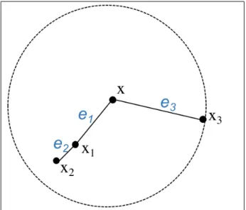
its distance is not large enoughx – from [18] . . . 5 1.2 LOF fails to detect outliers – from [65] . . . 6 1.3 Fork = 3, theSBN-pathofxis{x, x1, x2, x3}, theSBN-trailis{e1, e2, e3} 7

1.4 LOF assigns low score to q and r when clusters of different densities are present – from [38] . . . 9 1.5 Using ranks of friendship in social network to test the popularity – from [37] 10 1.6 Density-based algorithm assigns higher score to B than A – from [37] . . . 11 2.1 Independent Ensemble for Anomaly Detection . . . 25 2.2 Detection power of different algorithms [37, 38, 65] . . . 28 2.3 Toy example with three outliers . . . 29 2.4 Outliers may only be detectable on different projections of feature space [44] 29 2.5 Expected 5-NN distance for two spheres with radius r = 1, in a 2D

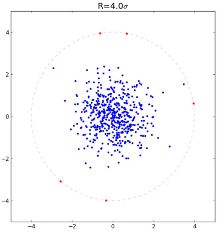
Eu-clidean space, containing 1000m (circles) and 100m (triangles) objects uni-formly distributed (0< m <1is the sampling rate) [75] . . . 33 2.6 An illustration for breadth first approach . . . 40 2.7 AUC Performance comparison over all methods for different datasets . . . 43 3.1 Framework for sequential ensemble method . . . 52 3.2 Multi-layer sequential model . . . 55 3.3 Synthetic dataset: outliers are generated on circle withR= 4σ . . . 58

3.5 Relationship between detection rate andβ on real-world data . . . 60

3.6 Performance of subsampling approach when samples are drawn from Dβ for different values ofβ, for three datasets. . . 62

4.1 2D example with 3 outliers . . . 72

4.2 Zoomed Score Histogram Example . . . 76

4.3 AUC Performance Comparison with Base Algorithm (LOF) over Differentk 79 4.4 AUC Performance vs. Number of Iterations . . . 82

5.1 An illustration of detecting the deviations in a data stream [8] . . . 85

5.2 An illustration of dataspace partition by one HSTree [64] . . . 86

5.3 A framework for streaming anomaly detection . . . 88

5.4 Variation of AUC with the number of noisy features in the syn-1 and syn-2 datasets . . . 90

5.5 Variation of AUC with the number of trees used in the syn-1 and syn-2 datasets . . . 91

5.6 Variation of AUC with the height of the trees used in the syn-1 and syn-2 datasets . . . 92

5.7 Numerical results for the number of trees and tree height . . . 96

5.8 A synthetic data where feature are interacted . . . 99

5.9 Two cases with outlier in different positions with respect to normal data . . 101

5.10 Performance comparison for our feature clustering method and random trees method on a synthetic dataset . . . 104

5.11 Performance comparison for our feature clustering method and random trees method for number of trees and height of trees on a synthetic dataset . 105 5.12 An illustration of individual representation used in EA . . . 108

liers from the other data points . . . 109 5.14 Evolution of solution quality with number of iterations, with different

strate-gies for synthetic dataset, whenpc= 0.6 . . . 111

5.15 Evolution of solution quality with number of iterations, for different values of crossover probability for synthetic data,pm = 0.2. . . 112

5.16 Evolution of solution quality with number of iterations, for different values of elitismewith different for synthetic dataset . . . 113 5.17 Results of using EA on a synthetic dataset . . . 114 5.18 Synthetic dataset with 4 clusters, outliers are inserted in between . . . 115

C

HAPTER

1

I

NTRODUCTION

Ensemble learning methods have many applications in machine learning and data min-ing area, especially in the context of classification. In classification problems, ensemble methods have been proven to be effective and robust over the base individual learners both empirically and theoretically. But few such works exist in the context of unsupervised anomaly detection. In this dissertation, we explore the application of ensemble learning methods for anomaly detection on both static and streaming datasets.

In this chapter, we first introduce the general concept of anomaly detection, then review some state-of-the-art detection algorithms which we apply (as components of ensembles) throughout this dissertation. Next, we describe the datasets and metrics we use to evaluate the algorithms described in this dissertation.

1.1

Anomaly Detection

Anomaly detection, also known as outlier detection, is one of the most widely studied among different research and application areas. In fact, the discussion of outlier detection in data sets can be traced back to the 18th century when Bernoulli questioned the prac-tice of deleting the outliers [14]. In recent surveys, the problem of finding anomalies is

often described asthe problem of finding patterns in data that do not conform to expected behavior[20]; or offinding data objects with behaviors that are very different from expec-tation[33]. Such patterns or data objects are the so-called anomalies or outliers.

Anomalies are usually associated with security threats, financial fraud, medical failure, system failures, etc. One of the most widely applicable areas for anomaly detection is detecting intrusions. For example, the financial losses by the respondent companies due to network attacks were over 130 million dollars in 2005 [52]; and according to a security report, more than 90% respondents experienced cyber-attacks in 2015 [56]. WannaCry ransomware attack, a worldwide cyberattack, launched on May 12 2017, was reported to have infected more than 2 million computers in over 150 countries [13, 21]. Therefore, detecting anomalies is a very critical problem.

Researchers have developed many anomaly detection methods over the years, based on statistics, machine learning, and information theory techniques. Each of the algorithms has an explicit or implicit assumption regarding what types of observations fall in the category of anomalies. Therefore, each algorithm has been developed to target a specific class of problem. However, in reality, the types of anomalies in a dataset can be of various kinds and hence cannot be detected by a single anomaly detection algorithm. To achieve better and more robust solutions, the application of ensemble learning is needed. Ensemble learning in the context of classification has been well explored both empirically and theoretically; Oza and Tumer [50] provide a survey of these techniques. However, as pointed out in [9, 74], the study of ensemble learning in the field of anomaly detection is still an open research problem. In the following, we first describe some of the existing state-of-the-art anomaly detection algorithms, and then introduce the current status of ensemble learning in anomaly detection.

1.2

Review of Existing Detection Algorithms

In this section we first describe recent density and rank based algorithms that we apply in ensemble methods.

The common theme among the three density based algorithms (LOF, COF, and INFLO) is that an anomaly score is assigned to an object based on density comparison of the object with its k nearest neighbors; an object is considered an anomaly if its anomaly score is greater than a pre-defined threshold. The other algorithms are based on the notion ofrank, and use the concept that ifk nearest neighbors of an object consider the object as one of their close neighbors, then it is less likely to be an anomaly.

1.2.1

Density Based Anomaly Detection Algorithms

The density based anomaly detection algorithms assume a symmetric distance function

dist, withdist(x, y) = dist(y, x), where x, y ∈ Dare two observations from the dataset. An important notion for various algorithms isNk(x), the set ofknearest neighbors (k-NN)

of a pointx ∈ D[18]. To find the k nearest neighbors, first define thek-distance of any observationxas:

k-dist(x) = dist(x, y),

wherey∈Dis thekth_{nearest neighbor ofxsuch that [18]:}

• |{z ∈D\ {x} |dist(z, x)< dist(y, x)}|< k, and

• |{z ∈D\ {x} |dist(z, x)≤dist(y, x)}|> k−1.

The set ofknearest neighbors ofxis defined as:

Nk(x) ={y ∈D\ {x} |dist(x, y)≤k-dist(x)}. (1.1)

pointsysuch thatxis among thek nearest neighbors ofy,i.e.,

Rk(x) = {y∈D|x∈Nk(y)}. (1.2)

Note thatNk(x)has at leastkobjects butRk(x)may be empty, becausexmay not be

in any of thek-NN sets of any of itsknearest neighbors.

LOF (Local Outlier Factor)

Local outlier factor (LOF), proposed in [18], captures the degree of outlierness of an object based on its local neighbors. It was proposed to solve a problem in global distance-based method [40] as illustrated in Figure 1.1, the distance-based method correctly identifieso1

as an outlier but fails to identifyo2 because its distance is not large enough. LOF, on the

other hand, assigns an outlier score for each object based on its local neighbors, and can successfully detect such outliers. The computed LOF score of an objectxis essentially the average of the ratio of the local reachability distance of an object with the average distance to the object’s k nearest neighbors Nk(x). To calculate the LOF score of each point in a

given datasetDof a givenkvalue, one should follow the steps given below:

• Calculate theknearest neighborhood setNk(x)of each objectx∈D.

• Calculate the local reachability density of each objectx∈D:

lrdk(x) =

" P

y∈Nk(x)reach-distk(x, y)

|Nk(x)|

#−1

wherereach-distk(x, y) = max{k-dist(y), dist(x, y)} is thereachability distance

Fig. 1.1: Distance-based based outlier detection algorithm fails to captureo2 because its

distance is not large enoughx – from [18]

• Calculate the local outlier factor (LOF) score of each objectx∈D:

LOFk(x) = P y∈Nk(x) lrdk(y) lrdk(x) |Nk(x)|

LOFk(x) captures the degree of x’s outlierness from its k-NN neighborhood. If x’s local reachability density is very low while its k nearest neighbors y ∈ Nk(x)

densities are high, then, x gets assigned a high LOF score, indicating that x is a potential outlier.

As a result, LOF score>1indicates that the object is potentially an outlier, whereas if LOF is≤1then the object’s local density is as large as the average density of its neighbors,

i.e., it is a non-outlier. LOF is considered to be the best method among NN approach, unsu-pervised SVM approach, and Mahalanobis based approach in the area of network intrusion detection [43]. Though it was proposed over ten years ago, it is still widely used in many recent applications. LOF has been used for fault process detection in a plant-wide process

monitoring system [45]; LOF was used to reduce the false alarm rate in their false data in the application of solar photovoltaic (PV) systems [71]; more recently, LOF was adopted in WiFall [69], an automatic fall detection system, to detect the anomalous wireless signal and to contribute to elders’ health care and facilitate injury rescue.

COF (Connectivity-based Outlier Factor)

After LOF, many other local kN N-based algorithms were proposed. Connectivity-based Outlier Factor (COF), proposed in [65], attempts to solve one of the deficiencies that LOF fails to detect outliers when the dataset contains clusters of different shapes, as shown in Figure 1.2.

Fig. 1.2: LOF fails to detect outliers – from [65]

To solve this problem, [65] proposed an alternative method for local density calculation which considers the “connectivity” – how an object connects to its neighbors, and use relative isolation to indicate whether an object is deviating from others. This connectivity is defined byset-based nearest path (SBN)andset-based trails (SBT). To calculate a COF score for each objectx∈Dfor a givenk, one can follow the steps given below:

B, as:

set-dist(A, B) = min{dist(x, y) :x∈A, y∈B}1

• Calculate thek nearestSBN-pathstarting fromx1: < x1, x2, ..., xk >such thatxi+1

is the nearest neighbor of set {x1, ..., xi}in set {xi+1, ..., xk}, for 1 ≤ i ≤ k −1.

In general, theSBN-pathis generated in an iterative expansion manner starting from

SBN(x) ={x}; in each iteration, the nearest neighbor object is added toSBN(x). In other words, theSBN-pathof objectxis an ordered list ofx’s nearest neighbors.

• The set-based nearest trail (SBN-trail) w.r.t a SBN-path p =< x1, x2, ..., xk > is

defined as a sequence < e1, e2, ..., ek−1 > such that ei = (y, xi+1) where y ∈

{x1, ..., xi}, |ei| = set-dist({x1, ..., xi},{xi+1, ..., xk}). |ei| is called the cost de-scriptionof edgeei. An illustration of aSBN-trailis shown in Figure 1.3.

Fig. 1.3: Fork = 3, theSBN-pathofxis{x, x1, x2, x3}, theSBN-trailis{e1, e2, e3}

• Calculate the average chaining distance fromxtoNk(x): AC-distNk(x) = 1 k−1 · k−1 X i=1 2(k−i) k · |ei| 1_{Note that this is not formally a metric since it does not satisfy the triangle inequality.}

the AC-dist is the average of the weighted distances in thecost description of the

SBN-trail. In theSBN-trail, if the edges closer toxhave larger cost descriptions than the edges far away fromx, then, the closer edges contribute more in the calculation ofAC-dist.

• Calculate the COF score for eachx∈D:

COFk(x) = |Nk(x)| ·AC-distNk(x)(x) P y∈Nk(x) AC-distNk(y)(y) .

The COF score of an object x indicates how x deviates from the objects it connects to, compared with its k nearest neighbors. An object with higher score is considered to be a potential outlier.

INFLO (INFLuential measure of Outlierness by symmetric relationship)

Another variation of LOF was proposed by [38], which addressed the problem that LOF fails to detect outliers when more than one cluster is present in the dataset, and different clusters have different densities. As shown in Figure 1.4, when q is slightly closer to a dense cluster than p, then p will be assigned a higher LOF score. INFLO proposes to use not only thek-nearest-neighborhood but also the reverse-nearest-neighborhood (RNN) (Rk(x)), defined in Equation (1.2). INFLO score is calculated as follows:

• CalculateNk(x)andRk(x)for eachx∈D.

• Calculate the local density of each object:

Fig. 1.4: LOF assigns low score toqandrwhen clusters of different densities are present – from [38]

• Get thek-influential-space for each objectx∈D:

ISk(x) =Nk(x)∪Rk(x)

• Calculate the INFLO score as:

IN F LOk(x) = P y∈ISk(x) den(y) |ISk(x)| ·[den(x)]−1

Therefore, for each object, INFLO compares its local density to that of both itskN N and

RN N.

1.2.2

Rank Based Anomaly Detection Algorithms

RBDA (Rank Based Detection Algorithm)

Rank Based Detection Algorithm (RBDA) [37] exploits the mutual closeness of an object to its neighbors. In Figure 1.5, for example, Jack and Eric rank each other high in their list of friends while Bob is not considered as friend by his friends. Therefore, Bob is not as popular in this social network. These personal friends are essentially the local nearest neighbors in the dataset, and the friendship rank measures how far away an individual

Fig. 1.5: Using ranks of friendship in social network to test the popularity – from [37]

deviates from its friends. This mutual closeness is measured by friendship in a social network, while it is measured by the distance function in a generic dataset. The following steps describe RBDA:

• CalculateNk(x)for each objectx∈D.

• For each pair of objects(x, y)∈D, the rank ofyrespect toxis defined as:

rx(y) =|{z :d(x, z)< d(x, y)}|.

Rank measures how ‘close’yis tox; if there are fewer observations betweenxand

y, then,yis ‘close’ tox,i.e.rx(y)is very small.

Fig. 1.6: Density-based algorithm assigns higher score to B than A – from [37] kN N: RBDAk(x) = P y∈Nk(x)ry(x) |Nk(x)| .

RBDA has an advantage in detecting outliers when clusters with different densities exist in the dataset, unlike the density based algorithm that misidentifies the point at a cluster boundary as an outlier as shown in Figure 1.6.

RADA (Rank with Averaged Distance Algorithm)

RADA [36] adjusts the rank of each objectx by the averaged distance from itsk nearest neighbors. The function for measuring outlierness of an objectxis defined as:

RADAk(x) =RBDAk(x)×

P

y∈Nk(x)d(x, y)

|Nk(x)| .

1.2.3

Statistical Methods

Statistical anomaly detection methods detect an anomalywhich is suspected of being par-tially or wholly irrelevant because it is not generated by the stochastic model assumed[11]. In general, a statistical anomaly detection model fits a statistical model for the normal ob-servations, and marks any observation that does not fit in with the given model as an outlier. Detailed discussion of statistical anomaly detection techniques can be found in [20,52]. We introduce one of the popular techniques in detail in this section, namely, the Gaussian Mix-ture Model.

Gaussian Mixture Model (GMM)

GMM is one of the most frequently used parametric models for detecting anomalies when there is no prior knowledge of the density distribution [42]. GMM is a probabilistic model which assumes that all observations are generated fromN gaussian distributions but with unknown parameters, known as the mixture components. Each multivariate component is represented by a parameter set

θi ={µi,Σi}

whereµiandΣiare the mean vector and the covariance vector for theithmixture model,

re-spectively. The set of parameters{θ1, ..., θN}is estimated using Expectation-Maximization

(EM) algorithm [23]. EM algorithm might converge to a local maximum; to overcome this problem, multiple trials of GMM are executed in our implementation.

1.2.4

Streaming Anomaly Detection Algorithms

A datastream is defined as an infinite sequence of data points [59]:

where dataxi arrives at timestampti. Recent research papers in [32, 59] discuss the

chal-lenges and open problems in detecting anomalies for streaming data. Anomaly detection techniques developed for datastreams should have the following features:

• online: an observation should be identified as an anomaly at the time it arrives;

• temporal context: an observation should be compared with its temporal context (e.g. within a time period);

• incremental learning: a detection model should be adjustable incrementally;

• concept drift: a model should be able to detect anomalies under the presence of distribution change; and

• multi-dimensional: a model should be able to apply fast detection on multi-dimensional datastreams.

Over the years, many online anomaly detection techniques have been proposed, including statistics-based methods [70] which incrementally learn a probabilistic model and deter-mine whether an observation is an anomaly compared to the learnt model. The incremental LOF [55] was the online version of LOF, which computes the neighborhood in an incremen-tal way, and reduces the time complexity for detection fromO(n2)toO(nlogn). Though many detection methods have been proposed, there are few ensemble methods on stream-ing data. The recent work proposed in [64] applies the concept of random forest in the context of streaming anomaly detection, and reports good performance in both accuracy and time complexity. We will discuss these streaming methods in detail in Chapter 5.

1.3

Ensemble Methods in Machine Learning

Ensemble methods are widely used in the field of data mining and machine learning, espe-cially in the context of classification and clustering. Ensemble methods are considered to

be among the best data mining techniques in many of the data mining competitions. Vitaly Kuznetsov said in NIPS 2014 that“This is how you win ML competitions: you take other peoples’ work and ensemble them together.”[4]. As a matter of fact, using ensemble meth-ods to solve data mining problems is becoming one of the most popular techniques. For example, in 2009 Netflix launched a 1 million dollar competition for user rating prediction and the team “The Ensemble” achieved the highest accuracy [5, 72]; in 2009-2011 KDD cups, all the first place and second place winners used ensemble methods [72]; the 2016 KDD cup winning team used the gradient boosted decision trees which is an ensemble method which combines the results of a collection of weak predictors, typically decision trees [60]. However, as Charu C. Aggarwal mentioned in [9], “Compared to the clustering and classification problems, ensemble analysis has been studied in a limited way in the outlier detection literature.”

A particular algorithm may be well-suited to the properties of one data set and be suc-cessful in detecting anomalous observations of the particular application domain, but may fail to work with other datasets whose characteristics do not agree with the first dataset. The impact of such mismatch between an algorithm and an application can be alleviated by using ensemble methods where multiple algorithms are pooled before a final decision is made. Mathematically, ensemble methods help by addressing the classical bias-variance dilemma, at least in the classification context.

Recently, a few researchers have studied ensemble methods such as anomaly detection and distributed intrusion detection in Mobile Ad-Hoc Networks (see Cabreraet al. [19]). Others have studied supervised anomaly detection using random forests and distance-based outlier partitioning (see Shoemaker and Hall [62]). In the semi-supervised case, one pos-sible approach is to convert the problem to a supervised anomaly detection by exploit-ing strong relationships between features; Tenenboim-Chekina et al. [66] and Noto et al. [49] provide two different approaches to accomplish this goal. Pevny et al.[54] pro-pose anomaly detector processing for a continuous stream of data, which requires high

acquisition rate, limited resources for storing the data, and low training and classification complexity. The key idea is to use bagging on multiple weak detectors, each implemented as a one-dimensional histogram. In these approaches the word ‘ensemble’ has a different connotation.

In this dissertation, we propose and evaluate different ensemble methods for anomaly detection on static and streaming datasets. We evaluate our methods with respect to many real-world benchmark datasets. We now describe the evaluation metric and datasets we use throughout the entire dissertation, then, discuss our contribution and summarize the content for each chapter.

1.4

Evaluation Metrics

In this dissertation, we mainly use Area Under Curve (AUC) as the evaluation metric. The details are described below:

AReceiver Operating Characteristic (ROC)was originally used for radar signal analy-sis during World War II [31], to measure the power of rader receiver operators [24]. It has a wide range of applications in signal detection [26], biomedical informatics [41], clinical medicine performance [76], etc. Detailed descriptions can be found in [27, 34]. More re-cently, ROC curve has become one of the most popular performance metrics in the area of machine learning [51], it plots the true positive rate vs. the false positive rate. The ROC curve provides an illustration of detection power in a 2-dimensional space, however, we of-ten need a single scalar value to simplify the evaluation process. Therefore, the area under the ROC curve (AUC) is used to reduce the ROC curve to a single-valued number [34]. A perfect detection algorithm reaches an AUC score of 1.0 while a random guess for two class problem is 0.5. In machine learning, the positive class is often considered to be the class of interest, therefore, in our work, positive class is the anomaly class (outliers), denoted asO, and the negative class is the normal class (inliers), denoted asI. While the set of predicted

outliers is denoted asOˆ, predicted inlier set is denoted asIˆ. Therefore, the True Positive Rate (TPR) and False Positive Rate (FPR) are calculated using:

T P R= | ˆ O ∩ O| |O| and F P R= |O ∩ I|ˆ |I| .

1.5

Dataset Descriptions

In this section, we describe first the benchmark static datasets we use for ensemble algo-rithms evaluation in Chapters 2, 3, and 4. Then, we describe the streaming datasets we use for Chapter 5.

1.5.1

Benchmark Static Datasets

• Abalone dataset (Abalone) [46] : This dataset was used originally for predicting the age of abalones from physical measurements. We keep the 7 numerical features and choose the minority classes as outliers, and downsampled the two major classes (class 9 and class 10) as the inliers.

• Smartphone-Based Recognition of Human Activities and Postural Transitions Data Set (ACT)[57] : This dataset collects data from 30 volunteers wearing smart-phones. There are three static postures (standing, sitting, lying) and three dynamic activities (walking, walking downstairs and walking upstairs), as well as postural transitions that occurred between the static postures (stand-to-sit, to-stand, sit-to-lie, lie-to-sit, stand-sit-to-lie, and lie-to-stand). The 3-axial linear acceleration and 3-axial angular velocity values from the sensors data are used for classification, with 561 features and 12 classes. To construct our outlier detection evaluation dataset, we consider the class with the least number of instances (sit-to-stand) as outlier points and the class with most number of instances (standing) as inlier points.

• EEG dataset (EEG)[46] : All data is from one continuous EEG measurement with the Emotiv EEG Neuroheadset. The duration of the measurement was 117 seconds. The eye state was detected via a camera during the EEG measurement and added later manually to the file after analyzing the video frames. It has two states: eye-close and eye-open. We downsample the eye-close class as the outlier class.

• Glass dataset (Glass)[39] : The original glass identification dataset from UCI ma-chine learning repository is a classification dataset. The study of classification of types of glass was motivated by criminological investigation. At the scene of the crime, the glass left can be used as evidence, if correctly identified. This dataset contains features regarding several glass types (multi-class). Here, class 6 is a clear minority class, as such points of class 6 are marked as outliers, while all other points are inliers.

• Ionosphere dataset (Iono)[46] : The Johns Hopkins University Ionosphere dataset contains 351 data objects with 34 features; all features are normalized in the range of 0 and 1. There are two classes labeled as good and bad with 225 and 126 data objects respectively. There are no duplicate data objects in the dataset. To form the rare class, 116 data objects from the bad class are randomly removed. The final dataset has only 235 data objects with 225goodand 10baddata objects.

• KDD 99 dataset (KDD)[35] : KDD 99 dataset is available from DARPA’s intru-sion dataset evaluation program. This dataset has been widely used in both intruintru-sion detection and anomaly detection area, and data belong to four main attack categories. In our experiments, we select 1000 normal connections from test dataset and insert 14 attack-connections as anomalies. All 41 features are used in experiments. The dataset is available at [3].

• Lymphography dataset (Lympho)[44] : The original lymphography dataset from the UCI machine learning repository is a classification dataset. It is a multi-class

dataset having four classes, but two of them are quite small (2 and 4 data records). Therefore, those two small classes are merged and considered as outliers compared to the other two large classes (81 and 61 data records).

• NBA Basketball dataset (NBA)[1] : This dataset contains Basketball player statis-tics from 1951-2009 with 17 features. It contains all players statisstatis-tics in regular season and information about all star players for each year. We construct our out-lier detection evaluation dataset by selecting all star players for year 2009, use their regular season stats as the outlier data points, and select all the other players stats in year 2009 as normal points.

• Packed Executables dataset (PEC) [53] : Executable packing is the most com-mon technique used by computer virus writers to obfuscate malicious code and evade detection by anti-virus software. This dataset was collected from the Malfease Project to classify the non-packed executables from packed executables so that only packed executables could be sent to universal unpacker. In our experiments, we select 1000 packed executables as normal observations, and insert 8 non-packed executa-bles as anomalies. All 8 features are used in experiments. The dataset is available at [2].

• Popularity (Pop) dataset[28] : This dataset contains features of articles published by Mashable in a period of two years. The original goal in the paper was to predict whether a news is popular or not in the social network. In the original paper [28], they threshold the number of shares to be 1400 to indicate whether a post is popular. For our experiments, we randomly down sampled 10 data points from the Popular class and mark them as outliers. Inliers are from the class non-popular.

• Statlog (Landsat Satellite) dataset (Sat)[46] : This dataset consists of the multi-spectral values of pixels in 3x3 neighborhoods in a satellite image. The original usage was to predict the class associated with the central pixel in each neighborhood.

To construct the outlier detection dataset, we downsampled class 4 (damp grey soil class) as the outlier, and class 7 (very damp grey soil class) as the inliers.

• Wine dataset[61] : This dataset has 13 features and 3 classes. To construct an outlier detection dataset, class 2 and 3 are used as inliers and class 1 is downsampled to 10 instances to be used as outliers. These data are the results of a chemical analysis of wines grown in the same region in Italy but derived from three different cultivars. The analysis determined the quantities of 13 constituents found in each of the three types of wines.

• Wisconsin Breast Cancer Dataset (WIS)[46] : This dataset contains 699 instances and has 9 features. There are many duplicate instances and instances with missing feature values. 236 instances are labeled as benign class and 236 instances as ma-lignant. In our experiments the final dataset consisted 213 benign instances and 10 malignant instances as anomalies.

1.5.2

Streaming Datasets

In this section, we describe the datasets we used for evaluating our streaming ensemble methods in chapter 5.

1. Http Dataset [64] : The KDD99 dataset can be divided into different subsets by the most basic feature ‘service’. Http is one of the subsets, in which the continuous features are transformed by taking a log function. This dataset is constructed using 567,497 ‘http’ service data and contains 0.4% anomalies.

2. CoverType Dataset[46, 64] The original ForestCover/Covertype dataset is used for predicting the forest cover types from the cartographic variables. The original dataset has 54 features including the quantitative variables, binary wilderness areas and

bi-T able 1.1: Summary of the benchmark datasets used for static data analysis Datasets No. of featur es Size of No. of outliers % of outliers Short description AB ALONE 7 492 5 1.02 the minority classes vs. class 9 & 10 A CT 561 1446 23 1.59 class sit-to-stand vs. class standing EEG 13 779 7 0.90 class 1 vs. class 0 GLASS 9 214 9 4.21 class 6 vs. the rest IONO 34 235 10 4.26 bad vs. good KDD 38 1012 12 1.19 intrusions vs. normal traf fic L YMPHO 18 148 6 4.05 tw o small classes vs. tw o lar ge classes NB A 17 578 24 4.15 all star players in year 2009 vs. the rest PEC 9 1008 8 0.79 malicious softw are vs. normal softw are popularity 10 1010 59 0.99 popular vs. non-popular ne ws SA T 4 474 36 0.08 class 4 vs. class 7 WINE 10 129 13 7.75 class 1 vs. class 2 and 3 WIS 9 223 10 2.23 malignant vs. benign

nary soil type variables. However, the outlier detection dataset is constructed by the 10 quantitative features. There are 286,048 data and 0.9% anomalies are inserted. 3. Polish Companies Bankruptcy Dataset [73] This dataset is collected from the

Emerging Markets Information Service (EMIS), which collects the information about emerging markets. The dataset contains financial information about the Polish com-panies from 2000-2013. We use the 5th year dataset which contains comcom-panies that are bankrupted after one year. This dataset has 64 financial features about 5910 total companies, of which, 410 companies were bankrupted during the predicting period.

1.6

Our Contribution

Anomaly detection ensembles has been categorized into two classes: independent learning and sequential learning, depending on how the base learners are used [9]. In this disser-tation, we explore and propose new algorithms for independent, sequential and adaptive learning. We study the application for ensemble methods in two contexts: static datasets and streaming datasets. For static datasets, we select the state-of-the-art unsupervised anomaly detection algorithms as our base algorithms and design different ensemble meth-ods. For streaming anomaly detection, we study both unsupervised and semi-supervised anomaly detection techniques.

• In Chapter 2, we first discuss the usage of independent ensemble methods for un-supervised anomaly detection. We consider three ensemble approaches using: (1) normalized scores, (2) rank aggregations, and (3) majority voting. We select 6 dif-ferent state-of-the-art unsupervised anomaly detection algorithms for ensembles, and our evaluation on different benchmark datasets show that using independent ensem-bles results in better performance than most of the base algorithms. In particular, using minimum ranking method achieves the best and most robust solutions. We then propose to use the bootstrapping idea for anomaly detection,i.e., taking

multi-ple sammulti-ples of the dataset, obtain anomalies for each sammulti-ple, and combine the results. This algorithm is comparable with existing works but has a lower computation cost. Finally, we discuss how to combine model-level ensembles and data-level ensembles, by boosting together to reach more robust decisions.

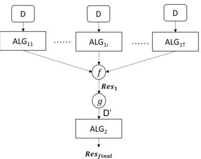
• In Chapter 3, we describe new sequential ensemble algorithms where the outputs of the first algorithm are further refined by another algorithm to detect anomalies. It has been argued that an anomaly detection algorithm performs better on a subsample of the dataset. We incorporate the sampling concept in proposed sequential methods. To select two (or more) algorithms, we propose to use the algorithms which have higher diversity among themselves as the base algorithms. In this chapter, we consider several minor variations of anomaly detection based on the sieve method which takes the output from one base algorithm to filter out the non-anomalous observations, then compare the suspect anomalies with a second algorithm.

• Boosting is considered as an example of iterative sequential learning; in particular, AdaBoost [29] has gained popularity in the classification context. However, boosting has not been used for unsupervised anomaly detection. In Chapter 4, we propose a novel adaptive learning algorithm for unsupervised outlier detection which uses the score output of the base algorithm to determine the hard-to-detect examples, and it-eratively resamples more points from such examples in a completely unsupervised context. Finally, we propose several methods to combine the results from each itera-tion.

• The random forests algorithm has shown better performance than single decision trees in the classification context [17]. Recently, a random forest approach has been proposed for anomaly detection [64]. However, this approach suffers from several deficiencies: (1) parameters are chosen based on empirical learning, and (2) this method does not perform well on high-dimensional data. In Chapter 5, we first

an-alyze the impact of parameters used in random trees, from both empirical and the-oretical points of view. Our main contribution is building better random forests for anomaly detection, achieved by : (1) determining the appropriate number of trees of heights based on our mathematical analysis, (2) feature clustering to build ran-dom forests without increasing the number of trees or tree heights, in order for the approach to be applicable to datasets with large number of features, and (3) apply-ing an Evolutionary Algorithm to further improve performance of the randomly built trees.

• In Chapter 6, we review and summarize the accomplishments of this dissertation. Then, we discuss the possible future works and improvements over the existing study.

C

HAPTER

2

I

NDEPENDENT

E

NSEMBLE

M

ETHODS

FOR

A

NOMALY

D

ETECTION

Independent ensemble methods combine the decisions from multiple base learners to reach a more robust and accurate final decision. In this chapter, we discuss the application of independent ensemble methods in the context of anomaly detection from both theoretical and empirical perspectives. We review and summarize some of the recent works using ensemble methods for anomaly detection. Then, we propose a bootstrapping algorithm based on the conclusion that using subsamples from the dataset will reach higher detection rate [75]. Results show that our bootstrapping algorithm provides competitive detection accuracy with much less computational cost. To combine the results from different base components, multiple combining strategies can be applied, including score based, ranking based and other approaches. While most existing works only apply a simple score aver-aging strategy, we explore the usage of rank aggregation and propose to apply a majority voting rule for the final result combination.

2.1

Independent Ensembles

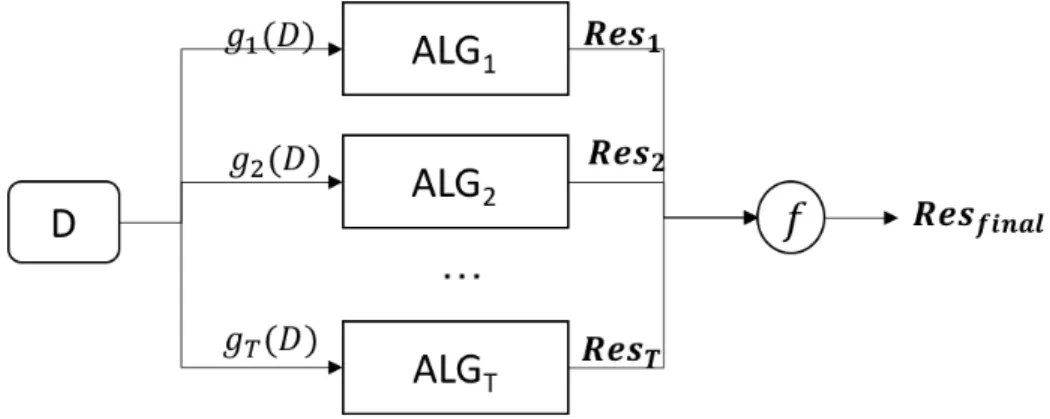
In ensembles, the final decision is jointly decided by multiple base components. Inde-pendent ensembles harness the independence between the base learners to achieve a lower error rate. The base components of independent ensembles can be constructed using in-stantiations of base algorithms, using subsets of datasets, and using different projections of dataset on feature space. After obtaining all the outputs from each component, the next step isfinal output combinationwhere the outputs are combined to achieve a better solution. An illustration of the independent ensemble approach is shown in Fig 2.1. There areT

base components, each of which could be a different algorithm, or the same algorithm but with different parameter settings or initiation [10]. The entire datasetD is taken, while a separate data transform functiongi is applied for theith base component. For example, if g is a random subsampling approach as in [75], thengi(D)is a random sample from the

datasetDand serves as the input for theithbase component. Each base component outputs a result vectorResi indicates the results made at componenti. A combination functionf is applied toResi, i= 1...T to make the final decisionResf inal; the combination function

could be averaging, minimum, etc.

2.1.1

Justification for Independent Ensemble Methods

The concept of using ensemble methods to achieve a better decision can be traced back to the famous Condorcet’s Jury Theorem [58] which was first proposed by the Marquis de Condorcet in his 1785 essay on theApplication of Analysis to the Probability of Majority Decisions [22]. The theorem says that when a jury ofT voters need to reach a decision by majority voting, if the probability of each voter being correct ispand the final decision being correct isp?_{, then it follows that:}

• Ifp > 0.5, thenp? _{> p.}

• If the number of votes approaches infinity, thenp? approaches to 1.0 ifp >0.5

The theory has two assumptions, that each vote should be independent and there should exist only two outcomes, for example, to convict or not. This can be easily adopted to independent ensembles for anomaly detection since:

• all votes (detection algorithms) are independent with respect to each other; and

• the decision outcome for anomaly detection falls into binary classes: whether an observation is an anomaly or is not.

As a result, from Condorcet’s Jury Theorem, it follows that applying independent ensemble methods for anomaly detection could lead to a more robust and stronger decision than the single detection result. However, Condorcet did not give a mathematical proof. A theoretical justification is provided by Hoeffding’s Inequality that as the number of base learners becomes very large, the generalization error goes to zero [72].

Consider a binary classification problem where the label of objectxfrom theith

classi-fier isHi(x)∈ {+1,−1}. Suppose we haveT classifiers which are independent with each

other. Definepas the probability that the decision made by one of the members in the jury is correct. As a result, each classifier has a classification error1−p. After combining these

T classifiers, the final decision for each object is represented as: H(x) = sign _XT i=1 hi(x)

The final decision makes an error if more than half of the T classifiers make errors. By

Hoeffding’s Inequality, the generalization error of an ensemble is [72]:

Error= bT /2c X i=0 T i (p)i(1−p)T−i ≤exp −1 2T 2(1−p)−1 2

This guarantees that as the number of base learners increases, the generalization error is exponentially decreasing.

2.1.2

Benefits of Ensembles - A Toy Example

In unsupervised anomaly detection, each algorithm makes an assumption about what is an anomaly. For example, in density-based detection algorithms, the observations in a low-density area are identified as anomalies. Fig 2.2 shows examples of the illustrations of data on which different algorithms are successful.

To show how to ‘cancel’ the bias of each algorithm in detecting anomalies, we construct a very simple toy example with three outliers, shown in Figure 2.3(a). Figure 2.3(b) shows the ROC curve for different algorithms. Each algorithm successfully captures 2 out of 3 outliers but fails to detect the other one. However, all outliers are captured by applying an ensemble using the minimum method which is defined in Equation (2.4) in Section 2.3.

2.2

Data Transformation

One of the requirements of the independent ensemble approaches is that the decisions made from each base component should be mutually independent. However, when we apply anomaly detection on the same dataset, the base components are inherently dependent due

(a) INFLO correctly detectsq (b) COF correctly detectso1

(c) RBDA correctly detects A

Fig. 2.2: Detection power of different algorithms [37, 38, 65]

to the reason that they share the same dataset. To reduce this dependence, different data transformation techniques can be applied. In this section, we review two of the existing data transformation functions including feature bagging [44] and random subsampling [75], then, we propose our new bootstrapping algorithm.

2.2.1

Random Feature Bagging

Feature bagging [44] is the first work to formally describe the application of an ensemble approach for unsupervised anomaly detection, motivated by two observations relevant to outlier detection: 1) outliers might only be detectable from a subspace or projection of feature space; 2) in high dimensional space, distances become sparse and outliers are dif-ficult to distinguish from the normal observations. This is shown in Figure 2.4, where the two outliers A and B can only be detected on different projections of feature spaces. This effect may occur when different types of outliers exist in the dataset. Another problem is the famous curse of dimensionality: in Euclidean space, as the dimensionality increases, the distances between data points are less distinguishable from each other [15]. When the dimensionalitydof the feature space becomes very large, the ratio of the difference in

min-(a) Toy example with 3 outliers (b) Evaluation: ROC Curves of independent methods (INFLO, LOF, RBDA and COF) vs. en-semble method (ens)

Fig. 2.3: Toy example with three outliers

imum and maximum Euclidean distance from data points to the centroid, and the minimum distance itself, tends to zero,i.e.:

lim d→∞E(

distmax−distmin distmin

)→0.

A recent article [63] shows that classification performance reduces significantly when in-creasing the dimensionality but not the number of training samples. To solve the

afore-Fig. 2.4: Outliers may only be detectable on different projections of feature space [44]

Al-gorithm 1. By contrast to the standard bagging approach, instead of randomly sampling from the data distribution, this approach draws random samples from the feature space and keeps all the data points. In thetthiteration, all data samples are preserved, butNtfeatures

are drawn uniformly from the entire feature spaceF S.

Algorithm 1Feature Bagging Approach

Data: DatasetDwithd−dimensionalfeature spaceF S Input: A set of anomaly detectorsA=A1, ..., AT

Result: A vector of anomaly scoresH

Normalize datasetD fort= 1, ..., T do

Nt=U {dd/2e, d−1};

F St= randomly pickNtfeatures fromF Swithout replacement;

Ht= apply detection algorithmAtonF St, get a score vector for each object;

end

Final output: H= COMBINE(H1, ..., HT)

The detection algorithm used in the original paper [44] is the same overT iterations, which is LOF. For the final COMBINE function, it discussed two combination methods: cumulative sum and breadth first approach, which we discuss in detail in Section 2.3. The paper showed that the approach outperforms LOF in many datasets especially when there exist noisy features; also cumulative sum outperforms breadth first combination.

2.2.2

Random Data Bagging

Bagging (Bootstrapaggregating) is one of the most used independent ensemble methods, and has been widely used in the classification context. Bagging was first proposed by Leo Breiman [16] where he proposed to improve the classification accuracy by building classi-fiers on random subsamples of training set. In Section 2.2.1, we have discussed Bagging

on the feature space. In this section, we discuss the Bagging approach by first summarizing Zimek’s [75] paper and then propose a new Bootstrapping algorithm.

Benefits from Detecting Outliers by Random Subsampling

The work in [75] proposed to use random subsampling methods for unsupervised anomaly detection to reduce the false detection rate. This method draws a random samplesfrom the datasetD, and for all observations x ∈ D, an anomaly detection algorithm is performed on{x} ∪D. This step is repeated multiple times and the final score is an average over all iterations. Zimeket al.[75] argues that by doing so, the benefits come from two aspects: 1. the density estimate for each sample will be more robust; 2 subsampling will increase the ‘gap’ between then. We now discuss the first benefit. Consider a scenario in which the true (but unknown) density distribution of inliers from datasetDare generated fromf, so that the estimated density of objectxis

ˆ

fD(x) =f(x) +D(x),

whereD is the sample error of estimation. When multiple samples are taken, the expected

density ofxis

E{fˆD(x)}=E{f(x)}+E{D(x)}=f(x) +E{D(x)}

Then, if the errorsD(x)are independent between multiple subsamples, the estimation of x will maintain the same order of true densityf(x) since in this case E{D(x)} is zero.

However, since there is no guarantee that the errors are the same over multiple samples, Zimek’s [75] paper argues that using their random subsampling method will not cause ranking inversion between inliers and outliers, but increasing the ‘gap’ between them, this is a more important finding as summarized in below.

expected Euclidean distance from a point to its k nearest neighbors, defined asE{kdist} is: E{kdist}=r k n 1/d

Now, suppose we have two spheres in the data space with n1 and n2 objects. Suppose n1 << n2, therefore, the sphere withn2 observations stands for the inliers, while the other

one contains the outliers since outliers lie in sparse area. The expectedkN N distances for the two spheres withn1andn2 objects are:

E{kdist1}=r k n1 1/d ; E{kdist2}=r k n2 1/d ;

Taking a fraction0< m <1of samples from the datasetD:

E{kdist0₁}=r k n1×m 1/d ; E{kdist0₂}=r k n2×m 1/d ;

The difference between the sampled distance and the original is:

∆1 =E{kdist01} −E{kdist1}=r k n1 1/d 1−m1/d m1/d (2.1) ∆2 =E{kdist02} −E{kdist2}=r k n2 1/d 1−m1/d m1/d (2.2) The expected kN N distance in the sampled space increases as a function of sampling ratem: ∆1 E{kdist1} = ∆2 E{kdist2} = 1−m 1/d m1/d (2.3)

Equations (2.1) and (2.2) justify that the expected k-N N distance after sampling will be larger for a sparse sphere than a dense one, which means that when n1 < n2, we have ∆1 > ∆2. This is equivalent to say that the sampling distances for outliers will grow

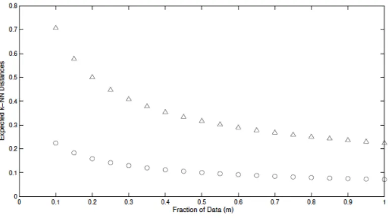
Fig. 2.5: Expected 5-NN distance for two spheres with radius r = 1, in a 2D Euclidean space, containing 1000m (circles) and 100m (triangles) objects uniformly distributed (0< m <1is the sampling rate) [75]

the denser areas. This effect can be seen in Figure 2.5, where two spheres with the same radius are represented, but the one shown with circles is denser than the one shown with triangles, and the expected distances after sampling grow faster for the sparse sphere as the sampling rate decreases. These findings justify the attempt to improve outlier detection with a sampling technique, Algorithm 2 describes this procedure.

Algorithm 2Random Subsampling

Data: DatasetD

Input: Sampling rate0< m <1; An anomaly detectorA Result: A vector of anomaly scoresH

fort= 1, ..., T do

Dt= randomly pickm× |D|data points fromD; forx∈Ddo

Ht(x)= anomaly score ofxobtained by applying detection algorithmAonx∪Dt; end end forx∈Ddo H(x) = _T1 PT i=1Ht(x) end

This approach uses the same base algorithm (LOF and its variants) for each iteration, and empirical results show that when the sampling fraction is 0.1, the anomaly detection performance is the best.

2.2.3

A Bootstrapping Approach – Proposed Algorithm

In statistics, bootstrapping techniques are commonly used for estimating the properties (mean, variance, confidence intervals, etc.) of the population using multiple samples [25]. Bootstrapping is a resampling method where multiple samples are drawn each time. The commonly used bootstrap method is the.632 method, which has been used to construct the training set and testing set for classification problems [33]. On resampling n points with replacementn times, 63.2% observations are presented in the training set while the other 36.8% observations are left for testing set. The number .632 comes from the approximate that(1− 1

n)

n _approachese−1 _{= 0.368 for a largen. In our method, we explore different}

resampling rates.

As shown in [75], applying distance-based outlier detection techniques on a subsampled data space will result in better performance than on the original dataset. They evaluate every point against the random subsample to avoid the chance that some objects will not be sampled. However, we argue that given enough number of random samples that the probability of missing an observation is very small; therefore, using a simple Bootstrapping approach will result in similar performance but be more efficient.

In our method, we select a subsample without repeating an observation. Hence, if we wish to select a proportion of m, 0 < m < 1, then the probability of not selection in a sample is(1−m). The probability that each point isnotdrawn fromT random samples is:

(1−m)T.

m×N >> N:

(1−(1−m)T)N.

We want this probability to be greater than1−δ, where0< δ < 1is a small number. To obtain the number of samplesT, we derive the following:

{1−(1−m)T}N _≥(1−δ) 1−(1−m)T ≥(1−δ)1/N

T ≥log_1−m{1−(1−δ)1/N}

For example, ifδ = 0.001,m = 0.1, andN = 1000, then we need to sample 132 times to achieve desired contraints.

The algorithm is very simple and shown in Algorithm 3. As shown later in the evalua-tion secevalua-tion, this simple Bootstrapping approach exhibits the aforemenevalua-tioned subsampling effect for improving anomaly detection, and is faster than the approach in [75] since one loop is eliminated from the algorithm.

Algorithm 3Bootstrapping Approach

Data: DatasetD

Input: Sampling ratem,0< m <1; A set of anomaly detectors{A1, ..., AT} Result: A vector of anomaly scoresH

fort= 1, ..., T do

Dt= by randomly selectm× |D|data points fromD;

Ht = anomaly scores of the datapoints inDt are obtained by applying detection

algo-rithmAt; end forx∈Ddo H(x) = _T1 PT i=1Ht(x) end

2.3

Final Results Combination

Most anomaly detection algorithms output a score for each object indicating the degree of that object being an anomaly. Although different algorithms output scores with different scales, we assume here w.l.o.g. that in all cases the larger the score, the higher the prob-ability that an object is an anomaly. How to combine the final scores to achieve a better result is very important in ensemble methods. Next, we review some of the most popular combination approaches and propose some new ideas.

2.3.1

Review of Earlier Methods

Feature bagging [44] is considered as the first ensemble approach for unsupervised anomaly detection [9]. In their approach, each base component is constructed by applying the same base algorithm on a random projection of the entire dataset on feature space. The pa-per evaluated two different combination approaches: cumulative sum and breadth first ap-proach. The cumulative sum approach is the same as averaging approach and is the most

popular combination method in most existing works [18, 44, 75]. The work in [18] eval-uates different combination methods such as using the maximum score output, using the LOF algorithm but with different values ofk, the number of nearest neighbors.

2.3.2

Different Types of Combination Methods

Score Based Combination Methods

The score averaging methodcombines anomaly scores for each observation, first normal-ized to be between 0 and 1. Letαi(x)be the normalized anomaly score of∈D, according

to algorithmi. Then the normalized score, averaged over all T base components, is ob-tained as follows: α(x) = 1 T T X i=1 αi(x).

The maximum score combinationmethod selects the maximum score output from theT

base components for each object. It was shown in [18] to perform better than the minimum score and averaging score approach.

α(x) =maxT i=1 αi(x)

Rank Based Combination Methods

Since each algorithm outputs anomaly scores in different scales, the required score normal-ization in a score-based combination method may be biased. Using rank based methods, we can overcome this problem.

The minimum ranking approach considers the minimum rank of each object as the fi-nal output, instead of using the score output. Let the anomalous rank of x, assigned by algorithmi, be given by:

A smaller rank implies that the observation is more anomalous. The minimum rank method assigns

rank(x) = min

1≤i≤Tri(x). (2.4)

Thus, if objectxis found to be the most anomalous by at least one algorithm, then the Min-rank method also declares it to be the most anomalous object. If all six algorithms give substantially different results, six different points may have the same rank.

The averaging ranking approach is similar to score averaging approach but considers the mean value of rankings over different base learners. The results obtained from this approach is not an integer anymore, we denote it asrank0. For any object x, the smaller

therank0(x), the more it is considered anomalous.

rank’(x) = 1 T

X

1≤i≤T ri(x).

Majority Voting Rule Methods

As discussed earlier, the majority voting rule has a solid foundation, supporting the argu-ment that the final combination reaches more robust decisions. Majority voting rules have been widely applied in the area of ensemble-based classification. However, the concept of majority voting has rarely been applied in the context of unsupervised outlier detection.

We propose to use a majority voting rule in which the basic idea is to throw away the outputs that are inconsistent with the rest of the base components. The challenge for designing a majority voting rule for unsupervised anomaly detection is that most anomaly detectors output a score instead of a clear decision. Since the number of anomalies (rare events) should be very small, we consider the ranked topτ%as the ‘true’ anomalies for

each base learner, therefore the decision for each objectxfrom theith_{component is:} Hi(x) =        1, ifri(x)≤τ%× |D| 0, otherwise. (2.5)

The final vote for each objectxis:

V(x) = T

X

i=1

Hi(x). (2.6)

The final decision for whether an objectxis anomalous is:

H(x) =        1, ifV(x)> T /2 0, otherwise. (2.7)

When Equation (2.6) is used, the ranks of objects should be in descending order,i.e., truly anomalous objects should have more 1’s than 0’s. A binary decision is output using Equa-tion (2.7). In our evaluaEqua-tion, we denote the method using EquaEqua-tion (2.6) asmajority, while the results obtained by Equation (2.7) asmajority binsince it output a binary decision.

The weighted majority voting approach: In the previous combination methods, each learner is assigned an equal weight. By doing so, each algorithm gets to vote for the final decision. However, given the assumption that most base learners are accurate at detecting anomalies, we assign more weight to the algorithms that agree more with the majority, hence there is a potential that the final decision reaches ‘closer’ to the truth. The weight assignment is based on the idea that if a base learner detects the same set of anomalies as the majority, it gets a higher weight than the one that often disagrees with the majority. To do so, we design a weight assignmentwi for each base algorithmias:

wi = P x∈DI(Hi(x), H(x)) P x∈DH(x) (2.8)

whereHi(x)is the decision of theith algorithm about whetherxis an anomaly, as defined

in Equation (2.5). H(x)is the decision reached by majority, as defined in Equation (2.7).

I is a function defined as:

I(x, y) =        1, ifx=y; 0, otherwise.

After such assignment, the algorithms that agree more often with the majority will be as-signed a higher weight than the others.

Other Combination Methods

The breadth first approach [44] sorts all the results obtained from different base algo-rithms in descending order, then selects the next object that has the highest anomaly score from all the base algorithms, in a breadth first searching order. An illustration is shown in Fig 2.6 with three base algorithms. ALG1 ranks x as most anomalous, z as second, and

y as the third, i.e. r1(x) < r1(z) < r1(y). For ALG2, it has r2(x) < r2(y) < r2(z),

while in ALG3,r3(z)< r3(x)< r3(y). To obtain the final result, the method ‘scans’ each

algorithm horizontally, in the figure. It finds the first anomaly obtained by ALG1, which is

x, then, it goes horizontally to ALG2, which isxagain, when it reaches ALG3, the second anomalyz is output; then, the method continues in the next row, z is already obtained as anomaly, so it is ignored, the third anomaly is y obtained by second row of ALG2. The final output isx, z, y.

2.4

Evaluation of Independent Ensemble Methods

k values from 1 to 25 for the kN N based algorithms. For GMM, we execute 25 random trials.

2.4.1

Performance over Different Combination Methods

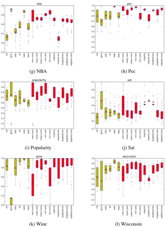
We plot the AUC scores (defined in Section 4.5) for variant individual and ensemble meth-ods, using boxplots for each dataset in Figure 2.7. We observe that among the individual base algorithms, RADA performs the best. The reason is that RADA itself is an ensem-ble which considers both distances and ranks for detecting anomalies. However, on some datasets,e.g., on NBA and SAT datasets, GMM performs better than RADA, which shows that if we choose RADA in all cases, then it does not perform well on these datasets. Using ensemble methods, on the other hand, might not beat the best individual base algorithm in all the cases, but it generates more robust solutions than the individual base algorithms. To summarize these results, we show the AUC scores for each dataset in Table 2.1, we observe that the combination methodmin rank generates the best AUC at 0.832±0.179 while the best base algorithm RADA generates 0.828±0.217. We also observe that though weighted methods are not the best, but they are perform better than the pure averaging methods:

weighted scorehas AUC at 0.791±0.214 while the pure mean scorehas 0.781 ±0.233;

weighted rankreaches 0.778± 0.202 whilemean rankhas 0.774± 0.204. Also, we ob-serve that when the base methods are all not performing well, for example, on Popularity dataset, while RADA gets an AUC of 0.628 and it is not the best among all the base al-gorithms, however, using our ensemble methodmin rankachieves an AUC at 0.843 which indicates that using an ensemble can achieve more robust results than a single algorithm.