Optimising Automatic Morphological Classification of Galaxies with
Machine Learning and Deep Learning using Dark Energy Survey
Imaging
Ting-Yun Cheng,
1
?
Christopher J. Conselice,
1
Alfonso Aragón-Salamanca,
1
Nan Li,
1
Asa F. L. Bluck,
2
Will G. Hartley,
3
,
4
James Annis,
5
David Brooks,
3
Peter Doel,
3
Juan García-Bellido,
6
David J. James,
7
Kyler Kuehn,
8
Nikolay Kuropatkin,
5
Mathew Smith,
9
Flavia Sobreira,
10
,
11
and Gregory Tarle
12
1School of Physics and Astronomy, The University of Nottingham, University Park, Nottingham, NG7 2RD, UK 2Kavli Institute for Cosmology, The University of Cambridge, Madingley Road, Cambridge, CB3 0HA, UK 3Department of Physics & Astronomy, University College London, Gower Street, London, WC1E 6BT, UK 4Department of Physics, ETH Zurich, Wolfgang-Pauli-Strasse 16, CH-8093 Zurich, Switzerland 5Fermi National Accelerator Laboratory, P. O. Box 500, Batavia, IL 60510, USA
6Instituto de Fisica Teorica UAM/CSIC, Universidad Autonoma de Madrid, 28049 Madrid, Spain 7Harvard-Smithsonian Center for Astrophysics, Cambridge, MA 02138, USA
8Australian Astronomical Optics, Macquarie University, North Ryde, NSW 2113, Australia 9School of Physics and Astronomy, University of Southampton, Southampton, SO17 1BJ, UK
10Instituto de Física Gleb Wataghin, Universidade Estadual de Campinas, 13083-859, Campinas, SP, Brazil
11Laboratório Interinstitucional de e-Astronomia - LIneA, Rua Gal. José Cristino 77, Rio de Janeiro, RJ - 20921-400, Brazil 12Department of Physics, University of Michigan, Ann Arbor, MI 48109, USA
Accepted 2020 February 13. Received 2020 January 15; in original form 2019 March 02
ABSTRACT
There are several supervised machine learning methods used for the application of automated morphological classification of galaxies; however, there has not yet been a clear comparison of these different methods using imaging data, or a investigation for maximising their effec-tiveness. We carry out a comparison between several common machine learning methods for galaxy classification (Convolutional Neural Network (CNN), K-nearest neighbour, Logistic Regression, Support Vector Machine, Random Forest, and Neural Networks) by using Dark Energy Survey (DES) data combined with visual classifications from the Galaxy Zoo 1 project (GZ1). Our goal is to determine the optimal machine learning methods when using imaging data for galaxy classification. We show that CNN is the most successful method of these ten methods in our study. Using a sample of∼2,800 galaxies with visual classification from GZ1,
we reach an accuracy of∼0.99 for the morphological classification of Ellipticals and Spirals.
The further investigation of the galaxies that have a different ML and visual classification but with high predicted probabilities in our CNN usually reveals an the incorrect classification provided by GZ1. We further find the galaxies having a low probability of being either spirals or ellipticals are visually Lenticulars (S0), demonstrating that supervised learning is able to rediscover that this class of galaxy is distinct from both Es and Spirals. We confirm that∼2.5%
galaxies are misclassified by GZ1 in our study. After correcting these galaxies’ labels, we improve our CNN performance to an average accuracy of over 0.99 (accuracy of 0.994 is our best result).
Key words: galaxies: structure – methods: data analysis – methods: statistical
? E-mail: [email protected] (KTS)
1 INTRODUCTION
The morphological classification of galaxies is a very important tool for understanding the history of galaxy assembly. It not only tells
us about the evolution of galaxies, but it can also reveal the stellar properties of galaxies, and thus their histories. Since the pioneering
work byHubble(1926), nearby galaxies can be easily and clearly
classified into two main types: early-type galaxies (ETGs), which include elliptical galaxies and lenticular galaxies, which are mostly massive, with older stellar populations, and no spiral structure; and late-type galaxies, which include spiral galaxies and irregular galaxies, often with spiral arms, and which consist of a younger population. These two types are the basic classifications of galaxies in local universe and have remained so for nearly a century.
Along with the data explosion by more and more survey
projects in astronomy, e.g. The Sloan Digital Sky Survey (SDSS)1,
the Large Synoptic Survey Telescope (LSST)2, the Dark Energy
Survey (DES)3(DES Collaboration 2018), etc, which will image
more than hundreds of millions of galaxies, the traditional manual classification analysis by experts is obviously impossible to deal with this enormous amount of data.
The series of the Galaxy Zoo projects (Lintott 2008,2011;
Willett 2013) are one of the most successful tool to solve the prob-lem of large scale morphological analysis. It allows amateurs to do the classification by answering a series of questions based on galaxy images. However, classification analysis is complex and dif-ficult such that background knowledge and experience are essential when doing it. In addition, while visual morphological classifica-tion with Galaxy Zoo is faster than for single individuals, it is also time-consuming. For example, the Galaxy Zoo Project spent around
3 years on obtaining the classifications of∼300,000 galaxies, due to
the need for so many individual classifications per object. DES and
LSST, for instance, would take on the order of>100 years to
clas-sify with the Galaxy Zoo project. Therefore, an efficient automated classification method by computational science is essential for the future of this field. The way forward is clearly through machine learning, although we are still learning the best ways to apply this to galaxy morphology and other areas of astronomy, e.g. star-galaxy
separation (Odewahn 1992;Weir 1995;Ball 2006, etc), the Galaxy
Zoo challenge (Chou 2014), the Strong Gravitational Lens Finding
Challenge (Metcalf 2019), etc.
The concept and application of machine learning in
computa-tional science have been around for some time (Fukushima 1980),
and the application in astronomy started in the 1990s. However, it has not been widely used in astronomy until the last few years due to the big improvement of the computation ability of comput-ers and the development of this technology. The first application of machine learning on morphological classification can be traced to Storrie-Lombardi(1992). They applied a neural network with an input layer of 13 parameters, e.g. stellar properties, brightness profile, etc., which gave an output of five different types of galaxies. Since then, a slew of studies in astronomy have appeared utilising
the technology of machine learning (e.g.Huertas-Company 2008,
2009,2011;Shamir 2009;Polsterer 2012;Sreejith 2017;Hocking
2017), neural networks (e.g.Mähönen & Hakala 1995;Naim 1995;
Lahav 1996;Goderya 2002;Ball 2004;de la Calleja 2004;Banerji
2010), and Convolutional Neural Networks (CNN) (e.g.Dieleman
2015;Huertas-Company 2015, 2018;Domínguez Sánchez 2018) for the morphological classification of galaxies.
There are now several different methods in machine learning used to carry out morphological classifications. However, although 1 https://www.sdss.org
2 https://www.lsst.org
3 https://www.darkenergysurvey.org/
Labels Machine Learning Algorithms 1 K-Nearest Neighbour (KNN) 2 KNN + Restricted Boltzmann Machine
(KNN+RBM)
3 Support Vector Machine (SVM) 4 SVM + Restricted Boltzmann Machine
(SVM+RBM)
5 Logistic Regression (LR)
6 LR + Restricted Boltzmann Machine (LR+RBM)
7 Random Forest (RF)
8 RF + Restricted Boltzmann Machine (RF+RBM)
9 Multi-Layer Perceptron Classifier (MLPC)
10 Convolutional Neural Network (CNN) Table 1.The list of machine learning methods tested in this study. machine learning have been highly developed for decades there is not a clear quantitative comparison between these different methods yet especially concerning imaging data. In our study, we carry out a comparison of the simplest classification – binary morphological classification of ‘Ellipticals’ and ‘Spirals’ (follows the classification of the Galaxy Zoo 1 project) – between several common methods
in machine learning (listed in Table1) using imaging data.
In previous studies, except for the application of CNN, there were very few studies which directly exploited imaging data when using other machine learning algorithms, such as neural networks or support vector machine. Therefore, we imitate the application of
face and hand-writing recognition in computational science (Bishop
2006) that directly input image pixels as features to all the methods
we compared for a fair comparison of different methods.
In this study we use DES imaging data which has better
res-olution and deeper depth than SDSS images (see Section2). With
our machine learning algorithm, these properties of DES data help us to build a larger, deeper, and better catalogue of galaxy morphol-ogy containing the largest sample to date. We therefore also discuss galaxies which ’fail’ in our training algorithms, and discuss how these systems are often misclassified in Galaxy Zoo. We also dis-cuss systems that have a low probability of being either an elliptical or a spiral and how these systems are visually classifiable on the DES imaging as lenticulars.
The arrangement for this paper is as follows. Section2
de-scribes the data resources, the procedure of pre-processing, and the datasets we use in this paper. The descriptions of each method are
discussed in Section3. We present the main results in Section4and
include a further discussion in Section5. The conclusion is shown
in Section6.
2 DATA SETS
For the images in this analysis we use the subset of Dark Energy Survey (DES) Year 1 (Y1) GOLD data - DES observation of SDSS
stripe 82, selected at magnitudei<22.5 and redshiftz<0.7 (
Drlica-Wagner 2018). DES data covers 5000 square degrees (∼1/8 sky)
and partially overlaps with the survey area of the Sloan Digital Sky Surveys (SDSS), but has a better seeing than the SDSS images from
Galaxy Zoo. Dark Energy Camera (DECam) (Flaugher 2015), the new installed camera used in DES, which is mounted on the Victor M. Blanco 4-meter Telescope at the Cerro Tololo Inter-American Observatory (CTIO) in the Chilean Andes, improved the quantum
efficiency in the infrared wavebands (>90% from∼650 nm to∼900
nm), and gives a better quality images for the observation of very distant objects than previous surveys with the spatial resolution of
0.00263 per pixel and the depth of
i=22.51 (DES Collaboration
2018).
A DES survey image has more than 500M pixels. Each tile is 1/2 sq.-deg. The coadd (tile) images are 10000 by 10000 pixels
in size with a pixel scale 0.00263. The total number of the data in
this subset is around 1.87 million galaxy stamps with photometric
redshift, and photometry information in 308i-band coadd images.
In order to train our machine learning algorithm, we match the DES data with the visual morphological classifications from the
Galaxy Zoo 1 project (GZ1, hereafter)4 (Lintott 2008,2011). we
only exploit the visual classifications which have agreements (votes
rates) over 80 percent and have been bias corrected by Bamford
(2009) for both Ellipticals and Spirals in GZ1. However, the
match-ing of DES data with visual classifications from GZ1 only gives 2,862 objects in total, with the number ratio between Ellipticals and
Spirals being 1 to 3. Their magnitude ranges from∼12.5 to 18 in
i-band, and the redshift z≤0.25 (peak at z∼0.1). To avoid overfitting
while carrying out the ML training, we apply data augmentation
in the pre-processing procedure in our study (Section 2.1.1). To
improve the performance of our machine learning methods, we ap-ply other techniques including feature extraction, i.e. Histogram of
Oriented Gradient (HOG) (Dalal & Triggs 2005) to extract other
informative features from galaxy stamps (Section2.1.3).
2.1 Pre-Processing
Before data pre-processing, we separate our 2,862 galaxies with DES data and the GZ1 classification randomly into training sets, and testing set, to prevent repeated galaxies in both sets. Our data pre-processing has four main steps: (1) Data Augmentation; (2) Stamps creation; (3) Feature Extraction; (4) Rescaling. The details are shown below.
2.1.1 Data augmentation
Data augmentation is of great importance while using pixel inputs
in machine learning. SinceDieleman (2015), data augmentation
by rotating images has been widely used within CNN for the mor-phological classification of galaxies. In this paper, we have 2,862 galaxies with visual classifications from GZ1, 759 Ellipticals and 2,103 Spirals, respectively, to train and test our methods. In order to prevent over-fitting during training, we rotate each galaxy image by 10 degrees differences from 0 to 350 degrees to increase the number of training samples. Hence, the available number of training
sam-ples increase to∼100,000. After rotation, we add Gaussian noise
to the rotated images (Huertas-Company 2015). This noise is small
enough to not to influence the visual appearance and structures of the galaxies (namely, remain the same visual classification), but it is big enough to make a detectable but change of pixel values.
Although data augmentation through rotating images is a well
known method used in machine learning application (e.g.Dieleman
2015;Huertas-Company 2015), the effect of these rotated images is 4 https://data.galaxyzoo.org/
unexplored. Therefore, we investigate the difference of performance between partially and fully using rotated images in the datasets in
Section4.2.
2.1.2 Creation of the galaxy stamps
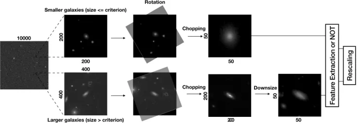
Fig.1shows the pre-processing procedure used in our study. Using
the galaxy catalogue from DES, we cut the coadd images with units of size 10000 by 10000 pixels into millions of galaxy stamps with sizes of 50 by 50 pixels. The size of galaxy stamp is based on the size distribution of galaxies in the DES Y1 GOLD data (stripe 82), where over 99% of galaxies are smaller than a threshold of 25 by 25 pixels. Therefore, the size of our stamp is 50 by 50 pixels, which is twice as large as the threshold in the size distribution of galaxies.
Fig.1shows that before chopping the stamp to the size of 50
by 50 pixels, we create the galaxy stamps with an initial size of 200 by 200 pixels when the galaxy size is smaller than 30 by 30 pixels, and 400 by 400 pixels when the galaxy size is larger than 30 by 30 pixels. For smaller galaxies, we rotate the 200 by 200 pixels stamps first, then reduce them in size to 50 by 50 pixels; for larger galaxies, we rotate 400 by 400 pixel stamps, reduce them in size to 200 by 200 pixels, then downsize them to 50 by 50 pixels by calculating the mean value of pixels in a size of 4 by 4 pixel cell. This procedure is designed to prevent empty pixel values showing up at the corner of stamps when we rotate images with non-90 degrees rotations.
2.1.3 Feature Extraction
In our study, we apply the Histogram of Oriented Gradients (HOG) on both our original and rotated stamps to investigate the impact of this feature extractor on supervised machine learning. HOG is a feature extractor which is able to extract the distribution of gra-dients with their direction from each pixel value. It is useful for
characterising the appearance and the shape of objects (Dalal &
Triggs 2005). It calculates the gradients of the horizontal (x) and vertical (y) direction of stamps. The magnitude and orientation of the gradient are calculated as below,
|G|= q G2x+G2y, θ=arctan G y Gx (1)
where|G|is the gradient magnitude of each pixel,Gxis the gradient
magnitude measured in x-direction,Gyis the gradient magnitude
measured in y-direction, andθ is the orientation of the gradient
for each pixel in the images. It then measures the contribution of gradients from each pixel in the cell with the size of 2 by 2 pixels, and uses a histogram to describe the contribution of gradient magnitude to each orientation of gradient. The input of HOG image is the direct output of this feature extraction process, and we rescale the pixel
value to the range between 0 and 1 (Section2.1.4). Examples of
HOG images are shown in Fig.2.
HOG is very popular within pattern recognition studies, e.g. human detection, face recognition, and handwriting recognition
(e.g.Dalal & Triggs 2005; Shu 2011; Kamble & Hegadi 2015,
etc); however, it is not popular yet in astronomy studies for the usage of machine learning algorithms. One of the applications is
the detection of gravitational lensing images (Avestruz 2018), and
a few previous works on the galaxy morphology (e.g. The Galaxy
Zoo challenge Chou 2014). However, none of these studies have
examined the influence of HOG on the performance of machine learning algorithms. In this study, we apply HOG on our images to
23 -11 1 14 26 39 51 63 76 88 10 27 -26 -23 -17 -6 18 63 154 337 700 14 27 -26 -23 -17 -6 18 63 154 337 700 14 35 -17 20 94 241 537 1123 2288 4641 9295 185 10000 10000 200 200 400 400
Larger galaxies (size > criterion) Smaller galaxies (size <= criterion)
50 50 35 -17 20 94 241 537 1123 2288 4641 9295 18 5 0 0.00099 0.003 0.0069 0.015 0.031 0.062 0.12 0.25 0.5 1 33 124 281 440 597 755 912 1069 1228 1385 15 200 200 0 0.00099 0.003 0.0069 0.015500.031 0.062 0.12 0.25 0.5 1 50 Rotation Chopping Chopping Downsize Fe at ur e E xt ra ct io n or N O T Rescaling
Figure 1.Pre-processing procedure pipeline. The pipeline starts from the initial coadd images, then we chop the coadd images into different sizes according to the size of galaxies. After rotation, we chop and downsize the images to the required sizes: 50 by 50 pixels. The details of the procedure is in Section2.1
Figure 2.Examples of images from Histogram Oriented Gradient (HOG) with the cell size of 2 by 2 pixels.Left: HOG images.Right: original images
in linear scale.Top: Spirals.Bottom: Ellipticals.
investigate not only the effect of it on automated morphological clas-sification of galaxies, but also the impact of it on the performance
of different machine learning algorithms (Section4.4).
2.1.4 Rescaling
Rescaling is a very important process in the application of ma-chine learning. Different galaxies have different brightness due to their different properties and their distances, so the pixel values of each image have significant variation between galaxies. This would cause difficulties for machine learning algorithms when defining the boundaries between different classes. Therefore, we rescale the pixel values of each image (raw and HOG images) to the range be-tween 0 and 1 through normalising by the maximum and minimum pixel value of each image. We are aware that intrinsic brightness can be a classification criteria, including surface brightness. However,
in this study we are interested in the structure only and not on other properties that might correlate with a class of galaxy such as surface brightness.
2.2 The datasets
In this study, we create 4 different datasets (see Table2). The first
two datasets (1 & 2) contain both the original images and the rotated images, and the last two (3 & 4) contain only the rotated images. This setting is used for investigating the influence of rotated images
on the performance (Section4.2).
On the other hand, the datasets 1 & 3 are unbalanced which contain more spiral galaxies than elliptical galaxies in the datasets while the datasets 2 & 4 have an equal number of spiral galaxies and elliptical galaxies in each dataset. We balance the number of each type by adding different numbers of rotated images to each type. For example, we rotate images of the Ellipticals 7 times, but only 2 times for the images of Spirals in dataset 2, and 3 times for both types in dataset 1. We use this setting to investigate the effect of the balance between the number of each type in training
samples (Section4.3). In addition, we also reduce the differences in
the number of total training samples between each dataset to reduce the probable bias from this.
On the other hand, we have 2 (or 3 in CNN) different types of input data (i, ii, iii). The first type (i) is the raw image with linear scale, and the second type (ii) is the HOG image from feature extraction. The third type, ‘combination input (iii)’, is special for CNN due to the characteristic structure of CNN that we can combine both the raw images (i) and HOG images (ii) as input without increasing the number of features. This is an new way to combine data using CNN whereas people used to restore the images with different colours in the third dimension of CNN in previous studies. We then also investigate the effect of this combination input (iii)
and compare it with the other two types (i & ii) (Section4.4).
For the testing set, we randomly pick 500 galaxies from 2,862 galaxies for each type (Ellipticals and Spirals). The rest of unselected galaxies are training set. Therefore, we have 1,000 galaxies in total for testing and the ratio between Ellipticals and Spiral is 1:1.
labels i (raw), ii (HOG), iii (combination, for CNN) 1 original images+rotated images E:S∼1:3, Training=10,448
2 original images+rotated images E:S∼1:1, Training=11,381
3 only rotated images E:S∼1:3, Training=11,448
4 only rotated images E:S∼1:1, Training=12,381
Table 2.The arrangement of training datasets in this paper. The content included in the datasets are shown in the second column, and the third column shows that the ratio between Ellipticals and Spirals and the total number of training data in each dataset.
3 MODELS OF MACHINE LEARNING
The concept of machine learning can connect with the invention
of calculators (Turing 1950) that we program machine to obtain
the information we want through the input numbers or characters (features). The breakthrough of visual pattern recognition in
ma-chine learning started fromFukushima(1980) which proposed a
hierarchical and multilayered neural network - Neocognitron. Ma-chine learning stood on the stage of astronomical applications since
the 1990s (e.g.Odewahn 1992;Storrie-Lombardi 1992;Weir 1995,
etc).
There are two main types of features, ‘parameter input’ and ‘pixel input’, that can be fed into machine. In the studies of galaxy morphological classification, the ‘parameter input’ is where we use parameters, which have clear correlations with galaxy types
(e.g.Storrie-Lombardi 1992;Naim 1995;Lahav 1996;Ball 2004;
Huertas-Company 2008, 2009; Banerji 2010; Huertas-Company 2011;Sreejith 2017). For example, the ‘parameter’ input can be
surface brightness profile, colour, C-A-S system (Conselice 2003),
Gini Coefficient (Abraham 2003), etc.
On the other hand, the ‘pixel input’ means that we treat each pixel of an image as a feature to feed machine learning algorithms. The ‘pixel input’ is the most straightforward feature used in two for machine to learn although it significantly increases the number of features for computation. However, it is uncommon in previous studies of automated classification of galaxy morphology to use
‘pixel input’ (e.g.Mähönen & Hakala 1995;Goderya 2002;de la
Calleja 2004;Polsterer 2012) until the application of CNN become
popular in recent years (Dieleman 2015;Huertas-Company 2015;
Domínguez Sánchez 2018).
We use ‘pixel input’ for each method in this study to investigate the effect of ‘pixel input’ on different machine learning algorithms
(Table1). Restricted Boltzmann Machine (RBM) (Smolensky 1986;
Hinton 2002;Salakhutdinov 2007), shown in Table1, is the simplest neural network with one hidden layer, which we treat as a feature
extractor for in this study (Section3.1).
All of the codes in this study are built onPython. The main
packages we use in this paper arescikit-learn5 (Pedregosa 2011)
for most of methods;Theano6,Lasagne7, andnolearn8for CNN.
3.1 Restricted Boltzmann Machine (RBM)
Restricted Boltzmann Machine (RBM) (Smolensky 1986;Hinton
2002;Salakhutdinov 2007) contains one hidden layer which is the 5 http://scikit-learn.org/stable/
6 http://deeplearning.net/software/theano/ 7 http://lasagne.readthedocs.io/en/latest/ 8 https://pythonhosted.org/nolearn/
simplest neural network architecture (more explanation for the
ar-chitecutre of neural network in section3.6). This is a useful
algo-rithm for dimensionality reduction and feature learning; therefore, in this paper, the RBM is used as a feature extractor to connect each feature. It extracts the features which are more interlinked with each other before we feed them to other machine learning algorithms. The combination of machine learning algorithms such as logistic
regression (Chopra & Yadav 2017) and RBM is actually widely
used in face and handwriting recognition.
In this study, the setting of RBM is identical amongst all
meth-ods that we apply a fixed learning rate (=0.001), 1,024 numbers
of hidden units, and 500 iterations for RBM in training, where the learning rate determines how far to move the weights each time to-wards the local minimum of loss function. The number of iteration is approximately determined by where the maximum of log-likelihood is shown.
3.2 k-Nearest Neighbours (KNN)
K-Nearest Neighbours (KNN) is the simplest non-parametric
ma-chine learning algorithm (Fix & Hodges, Jr. 1951;Cover & Hart
1967;Short & Fukunaga 1981;Cunningham & Delany 2007). This is one of the most common methods in pattern recognition and has several applications in clustering and classification problems (in
as-tronomy e.g.Kügler, Polsterer, & Hoecker 2015). The concept of
KNN is to find highly similar data, where similarity is defined by
the ‘distance’ in the feature space between data. Parameterkis the
number of nearest neighbours counted in the same group. This fac-tor controls the shape of the decision boundary for the distribution of data.
Increasing the value ofkdecreases the variance in the
classi-fication but also increases the bias of the classiclassi-fication. We chose
the value ofkby plotting the accuracy (Equation5) versus different
values ofk, and the value we ultimately use isk=5. The distance
metric for calculating the distance between each data is defined by theEuclidean metric.
3.3 Logistic Regression (LR)
Logistic Regression (LR) is a generalised linear model (McCullagh
& Nelder 1989) which uses the sigmoid function1+1e−x (or logistic function) to output the probability of classification. The application
in astronomy such asHuppenkothen(2017) studies the variability
of galactic black hole binary.
The combination of LR and RBM is commonly used in face
and handwriting recognition (Chopra & Yadav 2017). The
improve-ment of this combination is rather significant in LR while using ‘pixel input’ because of the characteristics of neural networks (See
section4).
3.4 Support Vector Machine (SVM)
The concept of Support Vector Machine (SVM) algorithm is to find a hyperplane with the maximal distance to the nearest data
for each type (support vector) (Vapnik 1995; Cortes &
Vap-nik 1995). In this study, we use a non-linear SVM, in
particu-lar, the Radial Basis Function (RBF) kernel function (Orr 1995):
® x,x®0 →K ® x,x®0 =ex p −γ ®x− ®x 0 2
. The detailed
introduc-tion of the SVM algorithm is given in AppendixA.
network due to the capability of dealing with high-dimensional data (Zanaty 2012). The application of this in astronomy is very popular, e.g.Gao, Zhang, & Zhao(2008);Huertas-Company(2008,2009); Kovács & Szapudi(2015). In this study, we use Nu-SVM which
was first introduced by Schölkopf(2002), and apply thePython
package NuSVC. The value of nu is determined by the Python
packageGridSearchCV(Hsu, Chang, and Lin 2003).
3.5 Random Forest (RF)
Random Forest (RF) is an ensemble learning method developed byBreiman(2001) which aggregates the results from a number of
individual decision trees to decide the final classification (Fawagreh
2014). Each tree is trained by a randomly picked subset from the
training set. The RF is a well known machine learning technique
applied in Astronomy using ‘parameter input’ (e.g.Dubath 2011;
Beck 2018) but the application that directly using pixel such as our study is untested.
We useRandomForestClassifierfrom thescikit-learn
mod-ule (Pedregosa 2011). The number of trees (n_estimators) used
in this study is determined by plotting the accuracy (Equation5)
versus different values ofn_estimators, and we ultimately use 200
trees. The maximal number of features to consider for each split (max_features) is equal to p
Nf, where Nf is the total number
of features. Each tree grows until all leaves are pure or all leaves contain the number of leaves less than 2.
3.6 Multi-Layer Perceptron Classifier (MLPC)
Multi-Layer Perceptron Classifier (MLPC) is a supervised
artifi-cial neural network with multiple hidden layers (Rosenblatt 1957;
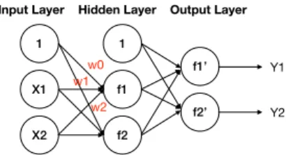
Fukushima 1975,1983). Hidden layers which have several hidden units are invisible layers between input and output layer in neural networks, and are used to connect input features with each other. Each hidden unit is an activation function calculated by the product of weights and input. Using a neural network with one hidden layer
as an example (Fig.3),X1 andX2 are input features, f1 and f2
are the activation functions of hidden units calculated by (using
f1 as an example) f1= f(w0·1+w1X1+w2X2), whereware
weights and f represents an activation function as well. Through
the calculation, it connects each input feature with hidden units by weights. Therefore, more hidden layers and more hidden units in each hidden layer can form more complicated connections of in-put features; however, the architecture with more hidden layers and hidden units is more time-consuming and can lead to overfitting problems. Similarly, the output layer also can be calculated from this concept.
MLPC uses a back-propagation algorithm (Werbos 1974;
Rumelhart, Hinton, & Williams 1986), which returns the error of predicted classification compared with the true label to the algo-rithm when the neural network is activated and the preliminary output is obtained. Algorithm adjusts the weights through the error
until the error is lower than the tolerance which we set 10−5. There
are two hidden layers and 1,024 hidden units for each hidden layer in MLPC method we used. The learning rate is fixed to 0.001. 3.7 Convolutional Neural Networks (CNN)
Convolutional Neural Networks (CNN) started from the design of
LeNet-5 (LeCun, Bottou, Bengio, & Haffner 1998). However, CNN
were not applied to the morphological classification of galaxies
Input Layer Hidden Layer Output Layer 1 X1 X2 1 f1 f2 f1’ f2’ Y1 Y2 w0 w1 w2
Figure 3.Illustration of a neural networks. This structure is for illustration only and this includes one hidden layer, and two hidden units. Two input features,X1 andX2, work with the activation functions,f1 andf2, then obtain the outputs,Y1 andY2.
utillDieleman(2015) in the Galaxy Zoo Challenge9. There are two
main differences between artificial neural networks (e.g. MLPC) and CNN. One is that CNN has convolutional layers which are able to extract notable features from the input images by applying several filter matrices, and the other difference is the dimension of the input. Most machine learning algorithms are designed for dealing with 1D array input (e.g. parameter input), but some of them (e.g. SVM and neural networks) are able to deal with higher dimension data. However, the input still needs to be reshaped to 1D arrays for SVM and MLPC. On the contrast, CNN is designed for image input with three dimension arrays which means that in addition to the image itself, CNN has an extra dimension to store more information of image such as colours (RGB).
Fig.4shows the architecture of CNN that we use in this study.
The input size of image is 50 by 50 pixels (Section2.1.2). We have
3 convolutional layers with filter sizes of 3, 3, 2, respectively, and each of them is followed with a pooling layer with size 2. These are then connected with two hidden layers with 1,024 hidden units for each layer. Additionally, two dropout layers are used to prevent overfitting, one follows the third convolutional layer (pooling layer), and the other comes after two hidden layers. The rectification of non-linearity is applied for each convolutional layer and hidden layer, and the softmax function is applied to the output layer to
get the probability distribution of each type (all from thePython
packagelasagne.nonlinearities). We useAdamOptimiser,Nesterov
momentum, and setmomentum=0.9according toDieleman(2015), and the learning rate 0.001 and maximum 500 iterations for the CNN training.
4 RESULTS
4.1 The evaluation factors for models
We use the Receiver Operating Characteristic curve (ROC curve) (Fawcett 2005;Powers 2011) to examine the performance of each
method and dataset. On a ROC curve they-axis is the true positive
rate and thex-axis is the false positive rate; therefore, the closer the
ROC curve gets to the corner (0,1), the better the performance is. The definition of true positive and the false positive are shown in
Fig.5in terms of the confusion matrix. Therefore, the true positive
rate (T PR) and false positive rate (F PR) are defined as below,
T PR= T P
T P+F N; F PR=
F P
F P+T N. (2)
The definition ofT PRis identical to ‘recall (R)’ in statistics which
represents the completeness that shows how many true types have 9 https://www.kaggle.com/c/galaxy-zoo-the-galaxy-challenge
50 50 2 (combination) 3 3 48 48 32 Max pooling =24x24 3 3 Max pooling =11x11 64 22 22 2 2 128 10 10 Max pooling =5x5 1024 1024 2 dropout = 0.5 dropout = 0.5
Figure 4.The schematic overview of the architecture of CNN. The architecture starts from an input image with size 50 by 50 pixels, then three convolutional layers (filter: 32, 64, and 128). Each convolutional layer is followed a pooling layer. Two hidden layers with 1,024 hidden units for each are following the third convolutional layer. One dropout (p=0.5) follows after the third convolutional layer and the other follows after the second hidden layer. At last, there are two outputs in our CNN, ‘Ellipticals’ and ‘Spirals’.
Figure 5.The confusion matrix. Thex-axis label is the predicted label and
they-axis label is the true label. The ‘0’ means negative as well as Ellipticals
type while ‘1’ represents positive signal and Spirals type in this study.
been picked, while ‘precision (Pr ec)’ indicates the contamination
which means how many picked types (predicted types) are true types. We are doing binary classification - positive: Spirals and negative: Ellipticals. Therefore, the recalls for Spirals and Ellipticals are shown below,
Pr ec= T P T P+F P; (3) R(1)= T P T P+F N; R(0)= T N T N+F P. (4)
Additionally, we also use the factor - the area under the ROC curve (AUC) as a performance evaluation for machine learning (Bradley 1997;Fawcett 2005). The meaning of AUC is the prob-ability that a classifier ranks a randomly chosen positive example greater than a randomly chosen negative example. This factor also indicates the separability - how well the classifications can be cor-rectly separated from each other.
4.2 The impact of rotated images
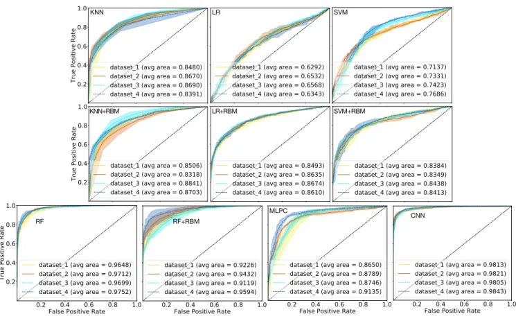
The ROC curves of each method and datasets are shown in Fig.6.
We show the results of raw images input (i) in this figure. Different colours represent different datasets such that the yellow, orange,
cyan, blue lines represents datasets 1, 2, 3, 4, respectively (Table2).
The datasets 1 and 2 contain both the original images and the rotated images, and the datasets 3 and 4 only contain the rotated images. Meanwhile, the datasets 1 and 3 have an unbalance number of each type, conversely, the datasets 2 and 4 have an identical number for each classification. The lighter colour shadings are the scatters defined by the minimum and maximum over three reruns. The black diagonal dashed line indicates a random classification.
First, the results of the LR and SVM methods, with and with-out combining with neural network, RBM show an improvement
for LR and SVM when combining with RBM in Fig.6. On the
con-trary, the performance of RF+RBM method shows slightly worse performance than the one of the RF method. Secondly, the scatters of the three reruns show small variance for each dataset, confirming the consistency of the reruns with each other. Additionally, as can be seen there are not large differences in the results between the different datasets. However, the slight shifts of the ROC curve occur within a few methods between the different datasets (e.g. MLPC). These are due to the slight differences in the total number of training
samples for different datasets (Table2). For example in MLPC, the
dataset 4 has the maximum number of training data within the 4
datasets used (∼12400 galaxies), so the performance of this dataset
is the best in MLPC; the datasets 2 and 3 have very similar num-ber of training data (the differences in numnum-ber is only 67), thus they have a similar performance to each other. The dataset 1 has
the least number of training data (∼10400 galaxies), therefore, the
performance is relatively worse. The shifts seen are also influenced by the condition of the balance between the ratio of each type (e.g. SVM and RF), for example, the datasets 1 and 3 are the unbalanced training data, so the shape of their ROC curve are similar to each other. This is also the case for the datasets 2 and 4. To summarise,
from Fig.6, data augmentation through rotated images works fair to
KNN KNN+RBM LR LR+RBM SVM SVM+RBM RF RF+RBM MLPC CNN
Figure 6.The ROC curve of each method and each dataset using the raw images input (i). The abbreviation of the methods are the same as Table1. Different colours are for the different datasets (Table2). Yellow, orange, cyan, blue are for dataset 1, 2, 3, 4, respectively. The lighter colour shading shows the scatters defined by the minimum and maximum of three reruns, and the lines inside are the averages of the three reruns. The black diagonal dashed line represents a random classification.
4.3 Balance or Unbalance?
Here we investigate the influence of the balance between the number
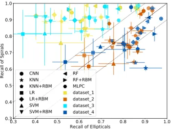
of each type in training data. Fig.7shows the recalls of Ellipticals
and Spirals for the different datasets using the different methods. The
colour representation is the same as the ROC curve of Fig.6, and
the different methods are marked by the different shape markers.
We obtain the value of the recall from equation 4for Fig.7by
averaging the values from the three reruns. Different pattern types represent different types of input. The colour-filled points are the raw images input (i) while the points with diagonal-filled marker are the HOG images (ii), and with dotted-filled marker are the combination input (iii). The black diagonal dashed line shows the condition that
R(0)=R(1)(Equation4), and the black dotted lines show that the
recall differences between these two types are within±0.1.
We observe that the unbalance training dataset 1 (yellow) and dataset 3 (cyan) are all above the upper dotted line which means that these two datasets generally have relatively higher recalls for Spirals compared to Ellipticals, and the differences of the recalls between Spirals and Ellipticals are larger than 0.1. For example, the result of the LR with the raw images input (i) (using the dataset 3 as an
example shown as the leftmost cyan square in Fig.7) has the recall of
(0.34, 0.81) for Ellipticals and Spirals, respectively. We also observe that the LR, LR+RBM, SVM, and SVM+RBM methods have more seriously unbalanced results than other methods when using the
unbalanced datasets (close to top-left in Fig.7). This situation is
due to the characteristics of these methods. For example, LR simply
uses logistic functions to determine the decision boundary which can be easily shifted by unbalanced number of each type. On the
other hand,Wu & Chang(2003) discusses the skewed decision
boundary of SVM caused by an unbalanced data such that the decision boundary is likely to be dominated by the support vector for the majority class.
On the other hand, most of the balanced dataset 2 (orange) and dataset 4 (blue) are located within two dotted lines which implies that these two datasets have similar recalls between Ellipticals and Spirals (the differences are smaller than 0.1). However, a few results of the balanced datasets in KNN have a higher recall of Ellipticals, but a relatively lower recall of Spirals (the orange and blue stars which are below the lower dotted line). KNN algorithm obtains the similarity between two images by calculating the ‘distance’ between
each pixel of two images (Section3.2). Spirals have various shapes
(e.g. different numbers of the spiral arms) while Ellipticals have a relatively simple appearance similar to one another. Therefore, it is easier for KNN to recognise Ellipticals than Spirals when we have the same numbers of both types within the training data.
We apply ten different common machine learning algorithms in this study and they show the consistent result in their balance except for KNN which we have discussed above; therefore, according to this discussion, the balance between the number of each type in training process is of great importance while using pixel input in most machine learning algorithms. In this figure, we also observe
Figure 7.The recalls of the Ellipticals and Spirals for all methods and the different types of the input data used. The colours represent the differ-ent datasets, while the differdiffer-ent shape markers are the differdiffer-ent methods. The different types of filled-points represent the different types of input. The fully-colour-filled markers are the raw images only (i), the diagonal-line-filled markers are the HOG images (ii), and those with dots are the combination input of the raw and HOG images (iii) which is only for CNN. The black dashed line represents the condition thatR(0)=R(1)
(Equa-tion4). The black dotted lines indicate that the differences in the recalls between these two types are within±0.1. The error bars are from the
stan-dard deviation of the three reruns.
that the CNN method with a balanced datasets obtains the best recalls of both Ellipticals and Spirals.
4.4 The effect of different types of input data
Here we show the comparison results between the different types
of input for each method (Fig.8). We have 2 (3 for CNN) different
types of input - the raw images (i) , the HOG images (ii), and the
combinations input (iii) (for CNN only). Different colours in Fig.8
indicate different types of input such that cyan, orange, and blue are for the raw images (i), the HOG images (ii), and the combination
input (iii), respectively. According to the discussions in section4.2
and section4.3, the results of the balanced datasets 2 and 4 are
basi-cally equivalent, and are better representations in our four datasets
(Table2). Therefore, we show the averages of the balanced datasets
2 and 4 after three reruns in Fig. 8, and the lighter colour
shad-ings show the scatters defined by the standard deviation of the three reruns.
Fig.8shows that the HOG images input successfully improves
the performance in most of methods, except for KNN. Although the HOG image is able to extract the characteristics of the morphologies according to the value of the gradients, it also loses some of the de-tailed information (i.e. the smaller fluctuations or gradients) and the smooth structure as well. Therefore, for KNN, the loss of the smooth structure in HOG images causes difficulties in determining the cor-rect decision boundary. This result can be significantly improved by combining KNN with RBM when using the HOG images.
On the other hand, we observe that the application of HOG images shows an unapparent effect when combining RBM in LR+RBM, SVM+RBM and RF+RBM. We infer that this phe-nomenon is caused because that the RBM interlinks with the HOG features which have less information in the images than the raw
images input. Therefore, it ‘annihilate’ the effect of RBM and HOG which leave an unapparent change in these three methods. This effect is shown in both MLPC and CNN as well such that the HOG images input shows only a slight improvement in these two methods as well. However, increasing the number of hidden layers or more neurons in the neural networks helps to connect the HOG features with each other. Therefore, the improvements with HOG images in MLPC and CNN are qualitatively better than LR+RBM, SVM+RBM, and RF+RBM. A more qualitatively significant improvement is shown in CNN when we combine both the raw images input and the HOG
images input (blue colour in CNN plot of Fig.8).
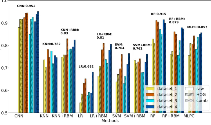
4.5 Comparison between methods
The definition of the accuracy used in Fig.9is shown below,
Accur acy= T P+T N
T P+F P+T N+F N, (5)
such the meaning of this is defined as how many successfully classi-fied samples there are out of all the samples tested. The comparison of the accuracy for the different datasets and the different methods
is shown in Fig.9. Through this figure we can observe the same
sit-uations as we have discussed in section4.4such that most methods
have a better performance when using the HOG images as input, except for the KNN where the HOG image input slightly reduces the performance, and the LR+RBM, SVM+RBM, and RF+RBM meth-ods which the HOG images input gives no apparent improvement in performance. We also make another comparison of efficiency
be-tween all methods (Table3). Most methods were run on the 2.3GHz
Intel Core i5 Processor with 16GB 2133 MHz LPDDR3 memory except for the ‘CNN (GPU)’ which was run on the NVIDIA GeForce GTX 1080 Ti GPU.
Interestingly, the performance of RF wins the performance of
MLPC with a faster computation time (Table3) using raw images
which was totally unexpected. The further investigation for the ca-pability of the RF on imaging data will be very helpful considering both the computing speed and a high accuracy the RF can reach. On the other hand, we can see that KNN and MLPC need less com-putation time but can reach a relatively good accuracy compared to other methods. Therefore, KNN and MLPC can be a good option when using pixel input. Additionally, although the KNN method has lower accuracy than MLPC, it applies raw images input which saves the preprocessing time that generates the HOG images (or other types of scaling).
The most successful methods when using pixel input in our
study according to both the ROC curve (Fig.8) and the comparison
of accuracy (Fig.9) between each method is certainly CNN. Both
of these two figures indicate that the HOG image input helps the
performance of CNN (Table4).
Additionally, we create a new way to utilise the third dimen-sion in CNN when we combine the raw image (i) with the HOG images (ii) which together we call a ‘combination input (iii)’. This shows a slight but qualitatively great improvement when using the combination input (iii) to do training in CNN (see CNN plot in
Fig.8). With the combination input (iii) and the balanced datasets,
we can reach∼0.95 accuracy with CNN using pixel input in this
study (Table4).
On the other hand,Sreejith(2017) proposes an ‘unanimous
disagreement’ indicating an object that all the classifiers agree with each other but disagree with the visual classification. In our study, we found only 3 galaxies out of 1,000 galaxies show an unanimous disagreement when considering all classifiers. These galaxies are
KNN KNN+RBM LR LR+RBM SVM SVM+RBM RF RF+RBM MLPC CNN
Figure 8.The ROC curve for different types of input within each method. Different colours are for different input types of data. Cyan, orange, and blue are for raw images (i), HOG images (ii), and combination input (iii), respectively. The lighter colour shadings show the scatters defined by the standard deviation calculated through three runs of the balanced datasets 2 and 4. The lines inside the shading are the averages of the three reruns of the datasets 2 and 4. The black diagonal dashed line represents a random classification. The subplot in the CNN method is the zoom-in area from 0.75 to 1.0 in y-axis and from 0.0 to 0.25 in x-axis.
all labelled as Spirals by the Galaxy Zoo 1 classification (GZ1) but classified as Ellipticals by our classifiers. We also visually con-firmed that these galaxies are indeed Ellipticals. This unanimous disagreement is more likely caused by the debias process applied in GZ1 to statistically adjust the population of galaxies at a higher redshift rather than a simple visual misclassification.
5 FURTHER DISCUSSION
We have already discussed some of our results in Section4while
presenting the results. In the last section we concluded that the best method of these ten supervised machine learning methods is Convolutional Neural Networks (CNN), the further analysis and the
discussion of CNN is essential for all future usage (Section5.1), as
well as the investigation of misclassification and galaxies with low
predicted probabilities (Section5.2).
5.1 Analysis of Convolutional Neural Network (CNN) Here we discuss in more detail the results of our CNN machine learning classification. We use a default criterion for the
classifica-tion in CNN such that the probability(p)>0.5 is the criterion for
classification; namely, Ellipticals or Spirals with p> 0.5 will be
classified as that type. When we change the criterion to p≥0.8,
Methods Training time Testing time accuracy KNN ∼0.2 sec ∼45 sec 0.782±0.027 (raw)
KNN+RBM ∼3000 sec ∼45 sec 0.830±0.007 (HOG)
LR ∼7-8 sec ≤1 sec 0.682±0.040 (HOG)
LR+RBM ∼3000 sec ≤1 sec 0.810±0.012 (HOG)
SVM ∼800 sec ≤8 sec 0.764±0.029 (HOG)
SVM+RBM ∼3000 sec ≤8 sec 0.762±0.001 (HOG)
RF ≤1 sec ≤5 sec 0.913±0.009 (raw)
RF+RBM ∼3000 sec ≤5 sec 0.870±0.031 (raw)
MLPC ∼18 sec ≤3 sec 0.857±0.010 (HOG)
CNN ∼3000 sec ≤5 sec 0.951±0.005 (comb)
CNN (GPU) ∼360 sec ≤5 sec 0.951±0.005 (comb)
Table 3.The comparison of the computing time (per∼1000 galaxies) for
each method. The ‘accuracy’ is the best accuracy shown in Fig.9. The first ten methods were run on the 2.3GHz Intel Core i5 Processor with 16GB 2133 MHz LPDDR3 memory, while the sixth method ‘CNN (GPU) was run on the NVIDIA GeForce GTX 1080 Ti GPU.
namely, any types withp≥0.8 are classified as the predicted type,
and if both types havep <0.8 then that galaxy will be classified
as ‘Uncertain type’. With this criterion, we separate our testing data into three different classes: Ellipticals, Spirals, and Uncertain. Using the combination input (iii), the accuracy of classification increases
Figure 9.The average accuracy (Equation5) of the three reruns versus each method with the different datasets and the different types of input shown. The y-axis is from 0.5 to 1.0. Colours represent different datasets such that yellow, orange, cyan, blue represents dataset 1, 2, 3, 4 (Table2), respectively. The different styles of shading are the different types of input data such that the fully-filled, the diagonal-line-filled, the dotted-filled represents the raw images (i), the HOG images (ii), and the combination input (iii), respectively. The labels above bars are the highest value of the accuracy for each method.
Input Types accuracy R01
raw (i) dataset 2: 0.924dataset 4: 0.906±±0.0130.018 0.9330.907 HOG (ii) dataset 2: 0.943dataset 4: 0.940±±0.0160.003 0.9400.940 comb (iii) dataset 2: 0.945dataset 4: 0.951±±0.0040.005 0.9470.953
Table 4.The comparison between the different types of input in CNN when using the datasets 2 and 4 (Table2). The total number of testing images is 1,000 galaxies. The definition of the accuracy is according to Equation5. The value ofR01is the recall value of Ellipticals and Spiral (Eqaution4) after taking a weighted average, and the value of this is shown in the table as the three reruns average ofR01.
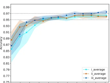
Secondly, increasing the number of training samples should in-tuitively improve the performance; however, we investigate whether this assumption is correct. We increase the number of our training samples by the rotated images, and keep the balance between the number of both types of galaxies. The maximum balanced number of the training data in our study is 53,663 (S: 26,839; E: 26,824).
In Fig.10, we observe that the increased rate of accuracy
re-mains basically positive, but this decreases as the number of training data increases. This shows that there is likely a maximum accuracy limitation within the CNN method for galaxy classification. This
accuracy R01 Nclassifiable Nuncetain dataset 2 0.974±0.004 0.973 912 88
dataset 4 0.974±0.003 0.973 927 73
Maximum 0.987±0.001 0.99 958 42
Table 5.The average result of the classification success with the classifica-tion criterionp>0.8 through using CNN for dataset 2, dataset 4 (Table2), and the result of the maximum available number of training data in our study with the combination input (iii) which includes both raw and HOG images. The total number of testing galaxies is 1,000. The definition of accuracy (Equation5) and the meaning ofR01are same as in Table4.Nclassifiable andNuncertainare the number of testing data which are classifiable (namely
p≥0.8) and uncertain (probabilities of both types(p)<0.8), respectively.
indicates that our combination input (iii) has a better performance than the other two types of input data as we increase the number of training data, and the combination input (iii) is the only one which
is able to reach over the accuracy of∼0.97 without any condition.
Therefore, we apply our maximum number of training data (53,663) with the combination input (iii) to do the training, and
combine it with the classification criterionp=0.8. We then obtain
a high accuracy of∼0.987 in the morphological classification of
Figure 10.The accuracy versus the number of training data with different types of input. Different colours show different types of input such that cyan, orange, blue are for the raw images (i), the HOG images (ii), and the combination input (iii), respectively. The lighter colour areas show the scatters of the standard deviation calculated by the five reruns, and the lines inside shadings show the average of the five reruns. The two dotted horizontal lines indicate the accuracy of 0.95 and 0.97.
probability sample fraction misclassification
p≥0.8 0.958 0.0142
0.7≤p<0.8 0.0184 0.239 0.6≤p<0.7 0.0302 0.132 0.5≤p<0.6 0.0114 0.368
Table 6.The fraction of the samples out of 1000 testing galaxies, and the fraction of misclassification within a certain probability range calculated by being divided by the sample number. The results are the average of five reruns.
5.2 Origin of Classification Failures
As shown in the above section, we are able to reach a high
clas-sification accuracy of∼0.987 by using CNN with the maximum
number of the training data with a combination of input (iii), and
the criterion of the probabilityp≥0.8. However, the<100
per-cent accuracy indicates that there are a few galaxies misclassified
but with high predicted probabilities (p≥0.8). On the other hand,
there are also a few galaxies (∼42 out of 1,000 testing galaxies)
which are non-classifiable (lower predicted probabilityp<0.8 in
both Ellipticals and Spirals). Table6shows the fraction of the
sam-ples within a range of probability (out of 1,000 testing galaxies), and the number of misclassification out of the galaxies within a probability range. It indicates that the classifications with higher
probabilities (p≥0.8) are much less often misclassified. However,
it also shows that galaxies with the predicted probabilities between 0.7-0.8 have a higher misclassified rate than the predicted probabil-ities between 0.6-0.7. This means that there are some galaxies with relatively higher predicted probabilities but which are misclassified by our CNN.
In this section, we define two types of failures by our CNN. One is the misclassification with the comparison to the Galaxy Zoo
1 classification with high predicted probabilities (p≥0.8), that are
galaxies which were classified with high probabilities with CNN but which later turned out to have a different classification in Galaxy Zoo. The other type of ‘failed’ classification are those galaxies with
low predicted probabilities (p<0.8 in both types) of being either
elliptical or spiral. We investigate the origin of these ‘failures’ in this section.
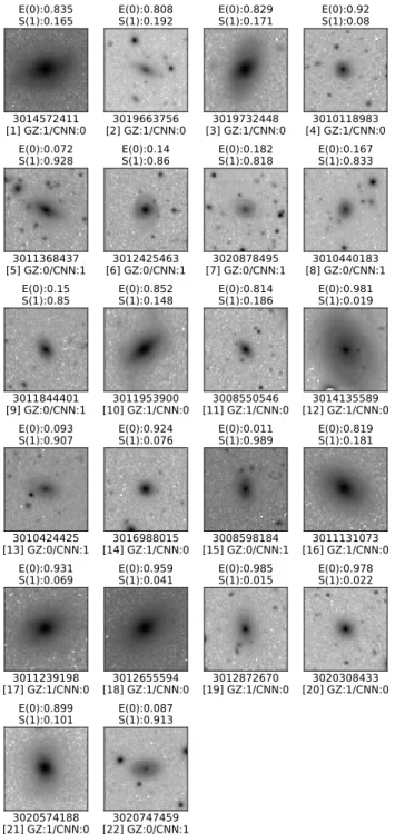
5.2.1 The failure with high probability: The misclassification of the classifiable galaxies
We rerun five times the best combination of our method (i.e. the CNN trained by the maximum balanced number of training data
and the combination input (iii), and classified by the criterionp=
0.8), and we then collect all the misclassification of the classifiable
galaxies from these five reruns together, obtaining 22 galaxies in
total (Fig.11). Misclassification in this sense is that what we get
from our CNN analysis differs from the Galaxy Zoo classification. Most of these 22 galaxies are repeatedly misclassified between these
five reruns, in Fig.11, objects 1-7 only show up once, objects
8-17 are repeated more than twice, and objects 18-22 are repeatedly showing up in five reruns. There are two main probable reasons for these misclassifications with a high probability through our CNN method. One is that we use the galaxy images with linear scale (including HOG images) on our CNN training, so in some cases, even if it shows the feature of Spirals in logarithmic scale, it is just a point source, a round object, or a large bright area in linear scale. Therefore, they prefer to be classified as Ellipticals rather than Spirals in our CNN. This will be further discussed in the
section5.2.3.
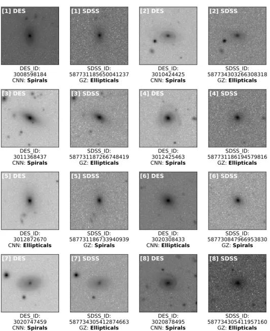
The other reason for the differences is due to misclassifications by the Galaxy Zoo 1 (GZ1). We apply visual classifications which have over 80% agreement between volunteer classifiers in the GZ1 catalogue in which we use to label our DES data. When we compare the SDSS imaging to the DES imaging, we can see some GZ1 classifications based on the SDSS data were simply wrong. Some
examples are shown in Fig.12. Most of them are revealed to be
misclassifications due to the better resolution and deeper depth of the DES data than the SDSS data. With higher resolution of the DES data, we reveal more detailed structure than the SDSS data (e.g the
number 4 and 8 in Fig.12which show clear spiral structures in the
DES data but nothing in the SDSS data). We will further discuss
this in Section5.2.4.
On the other hand, we also discover that some galaxies with large, bright, and oval structure are easy to misclassify using our method. These galaxies are lenticular galaxies when examined on the DES imaging. The main reason for their misclassifications is because there is not a class for lenticular galaxies in the Galaxy Zoo project. Lenticular galaxy is difficult to see by visual classification and typically requires high resolution and deep imaging, even for nearby galaxies. Some of them are therefore classified as Spirals, and some of them are recognised as Ellipticals in the GZ1 catalogue.
The details will be discussed in the next section (Section5.2.2) as
most of these galaxies generally have lower predicted probabilities of being either elliptical or spiral.
5.2.2 The failures at low probability: Uncertain type
In this section, we investigate the galaxies with lower predicted
probabilities (p<0.8) for classification as either elliptical or spiral
in the five reruns of our best method. The majority of the samples with lower probabilities are repeated between five reruns, and some
Figure 11.The misclassified galaxies with high probabilities (p ≥0.8)
comparing the classification of Galaxy Zoo 1 and our CNN. On the top of the images shows the probabilities of being Ellipticals, E(0) and Spirals, S(1) by our CNN. The line below the image shows the ID number of the galaxies in Dark Energy Survey (DES), and the second row shows the classifications by Galaxy Zoo and our CNN.
of them also show up in the previous section (Section5.2.1) which
are misclassified but with high probabilities. The probabilities of these galaxies vary significantly between each rerun.
The appearance of these galaxies can be separated into two types. One type are the galaxies which look large, oval, and bright (Top 1-12in Fig.13), and the other type are those which do not
combination input(iii)
log image +log image
accuracy R01 accuracy R01
dataset 2 0.950±0.006 0.947 0.952±0.006 0.950
dataset 4 0.954±0.004 0.953 0.964±0.007 0.967
Maximum 0.973±0.002 0.970 0.971±0.005 0.973
Max (p=0.8) 0.987±0.004 0.987 0.987±0.003 0.987
Table 7.The comparison of the accuracy (Equation5) and the recalls (Same as Table4) between the inputs of the log images and the combination of log images and combination input (iii) by using the dataset 2, dataset 4 (Table2), and the maximum number of training data.
appear this way, e.g. galaxies which are relatively fainter or with large bulge and spiral structure at the same time, or the target galaxy
is shifted significantly away from the centre of the image (Bottom
1-12in Fig.13).
The galaxies with large and oval structure are lenticular
galax-ies which we discussed in the previous section (Section5.2.1). As
discussed there is not a lenticular galaxy class in the GZ project, nor can these types be easily seen in SDSS data, therefore, the classifi-cation of these galaxies in the GZ1 catalogue are such that half of them are classified as Spirals, and half of them are classified as El-lipticals. Because lentinculars are neither spirals or ellipticals, their structure confuses our CNN such that it gives lower probabilities for these galaxies to be of either type. This is a ’rediscovery’ of lenticu-lars, and shows the power of machine learning for discovering new types of galaxies, as we did not expect this to occur.
5.2.3 Combined with logarithmic scale images
According to the discussion in the section5.2.1, we investigate
the impact on our classification with CNN when using images with logarithmic scale (hereafter, log images) to train our CNN algorithm
by using the datasets 2 and 4 (Table2). In addition to the log images,
we also combine the log images with our combination input (iii) as the input to train our CNN. The comparison of the results are shown
in Table7.
Comparing Table7with Table4shows a significant
improve-ment when using the log images, and the combination of the log images and our combination input (iii) shows a better accuracy than just using the log images as input.
However, comparing Table7with Table5shows that there are
not significant differences in the performance from log images input to the other three types of input, (i), (ii), (iii), when we train our CNN through the maximum available number of the training data. This means that there is an intrinsic limitation of our method. This
limitation can also be seen in Fig.10in Section5.1.
Therefore, we conclude that although adding the log images as input helps the performance, it still has no apparent difference from our result when we apply the maximum number of training data to our CNN.
5.2.4 The advantage of Dark Energy images and the misclassifications by Galaxy Zoo project
We have discussed the incorrect labels by Galaxy Zoo in previous sections. As discussed, the main reason to reveal the misclassifica-tion by SDSS imaging Galaxy Zoo is because of the better resolumisclassifica-tion
Figure 12.Examples of the incorrect label from GZ1 with SDSS imaging. The figures under each number show the galaxy images of DES and SDSS, and their ID numbers. The label of ‘CNN’ shows the predicted label from our method, and which of ’GZ’ shows the label from the Galaxy Zoo 1 catalogue.
(0.00263 per pixel) and deeper depth of DES data (i=22.51) (DES
Collaboration 2018).
These wrong labels not only influence the results of our CNN, but also contaminate the training set. Therefore, we remove the potential misclassified galaxies from the training set. We purify our training set by excluding the suspected misclassified galaxies then
use the criteria shown in Table8to confirm or dismiss our suspected
misclassifications. We then rerun our CNN classification five times on each new training set and obtain five new CNN models on the new classifications. After carrying out this purification twice, and then retraining and updating our list of suspects, we obtain two lists of these galaxies: one is the confirmed misclassified galaxies by the Galaxy Zoo, and the other are the suspected misclassified galaxies.
The images of these systems are shown in Fig.14and Fig.15.
There are∼2.5% misclassified galaxies in the Galaxy Zoo 1
cata-logue out of 2,800 in our study as revealed by using DES images
and our CNN, and∼0.56% are suspected candidates in our study.
We then correct our training set according to these two lists. We change the label of the confirmed misclassified galaxies, and ex-clude the suspected misclassified galaxies from the training set, then do the training with the maximum available number which is 53,141 galaxies in total (E: 26,344; S: 26,797). We then change the label of the confirmed misclassified galaxies in the testing set as well.
The results are shown in Table9. The first row of Table9is
the testing result excluding 8 suspected misclassified galaxies out of 1,000 testing galaxies. Compared this result with the results in
Table5, our new models predict the highest accuracy, and end up
having a resulting fewer number of uncertain type (about half the
original number) than the previous results. Therefore, Fig.16shows
the best testing result in our study. In this result, we change the label of the confirmed misclassified galaxies and exclude the suspected misclassified galaxies in testing set. We obtain the accuracy of 0.994
Figure 13.Examples of the galaxies with low probabilities of classification as either spiral or elliptical.Top 1-12:these objects are turned out to be
lenticular galaxies (S0) in cluster inspection.Bottom 1-12:the other types
of galaxies.
Criteria:
Confirmed (1) Appearing≥4 times in total failures.
(2) Appearing at least once in the high-p failures. Suspected (1) Appearing≥2 but≤4 times in total failures.
(2) Does not satisfy the criteria for ‘confirmed’. Not misclassification (1) Appearing≤1 time in the test of new models
Table 8.The criteria for selecting the suspected misclassified galaxies by the Galaxy Zoo project and purifying the training set.
for the best model within five reruns, and the average accuracy of five reruns is 0.991.
The second and third rows of Table9show the results including
suspected galaxies which retain the initial label from the Galaxy Zoo in test and change the label of them to the opposite label, respectively. We have lower accuracy in these two conditions than
accuracy R01 Nclassifiable Nuncetain No suspected galaxies 0.991±0.003 0.990 976 16
with suspected galaxies 0.989±0.001 0.990 981 19
label changed 0.987±0.003 0.986 981 19
Table 9.The testing result after using the purified training set. The meaning of each column are same as Table5. There are 8 suspected misclassified galaxies out of 1,000 testing galaxies. The first row is the testing result excluding suspected galaxies. The second row shows the result with the suspected galaxies which retain their initial labels from the Galaxy Zoo catalogue. The third row is the result with the suspected galaxies but their initial labels changed – for instance, the label changes to Elliptical if the initial label was Spiral.
the result of the first row. This indicates that part of our suspected galaxies have incorrect labels in Galaxy Zoo catalogue, and part of them are not, based on our CNN. Some examples of the successful
classifications by the purified CNN training are shown in Fig.17
and Fig.18.
6 CONCLUSIONS
In this study, we have examined ten supervised machine learning methods to determine the most successful method for classifying galaxies into ellipticals and spirals using only pixel input on a single
band (i-band). As part of the investigation, we have also tested how
using rotated images with various angles of rotation with 10 degrees increments to augment our data influences on our classification. In addition, we also confirmed that the balance between the number ratio of each type is rather important when using pixel input in machine learning.
We show that the machine learning algorithms, Logistic Re-gression (LR) and Support Vector Machine (SVM) improve the performance of machine learning when combining with neural net-works features, such as Restricted Boltzmann Machine (RBM). However, we find that using the image input along with the the His-togram of Oriented Gradient (HOG image) helps the performance in most methods, except for k-Nearest Neighbour (KNN). We also ob-serve that the application of HOG images gives less help when combining with a neural network (e.g. LR+RBM, SVM+RBM, RF+RBM) because the RBM interlinks the HOG image features which have less information than the raw images. However, increas-ing the number of hidden layers and neurons qualitatively helps the connection between the HOG image features according to the per-formance of Multi-Layer Perceptron Classifier (MLPC) and Con-volutional Neural Networks (CNN).
According to the Receiver Operating Characteristic (ROC) curve, the computing accuracy and the efficiency of each method, the performance of RF is comparable with a neural network (i.e. MLPC) with a faster computation time. In addition to RF, both the KNN and MLPC are alternative options can be considered when us-ing pixel input because both of them have a relatively good accuracy with much less computing time than other conventional machine
learning algorithms (e.g. LR, SVM) shown in this study (Table3).
The most successful method within the ten methods we test is the Convolutional Neural Networks (CNN) with the combination input of raw images and HOG images and when using a balanced training
data. Through this we are able to reach an accuracy of∼0.95 using
∼12,000 galaxies (including rotated images) as the initial training
Figure 14.The confirmed list of the misclassified galaxies in the Galaxy Zoo 1 catalogue. The first row underneath the images is the ID numbers of galaxies, and the second row shows the classification by Galaxy Zoo (GZ) and our CNN (CNN).