Least Squares Support Vector Machine with Self-organizing Multiple Kernel
Learning and Sparsity
Chang Liua, Lixin Tanga and Jiyin Liub
a Institute of Industrial and Systems Engineering, Northeastern University,
Shenyang, Liaoning 110819, China
b School of Business and Economics, Loughborough University, Leicestershire LE11 3TU, UK
Abstract
In recent years, least squares support vector machines (LSSVMs) with various kernel functions have been widely used in the field of machine learning. However, the selection of kernel functions is often ignored in practice. In this paper, an improved LSSVM method based on self-organizing multiple kernel learning is proposed for black-box problems. To strengthen the generalization ability of the LSSVM, some appropriate kernel functions are selected and the corresponding model parameters are optimized using a differential evolution algorithm based on an improved mutation strategy. Due to the large computation cost, a sparse selection strategy is developed to extract useful data and remove redundant data without loss of accuracy. To demonstrate the effectiveness of the proposed method, some benchmark problems from the UCI machine learning repository are tested. The results show that the proposed method performs better than other state-of-the-art methods. In addition, to verify the practicability of the proposed method, it is applied to a real-world converter steelmaking process. The results illustrate that the proposed model can precisely predict the molten steel quality and satisfy the actual production demand. Keywords: Least squares support vector machines, Self-organizing multiple kernel learning, Sparse selection, Differential evolution.
1 Introduction
Since the 1950s, several scholars have focused their research interests on machine learning [1], which has been widely applied to artificial intelligence fields such as pattern recognition, signal processing, image interpretation, and intelligent control. Based on the self-learning capability with historical experience, a deep exploration of machine learning has gone beyond computer science and has been carried on to biomedicine [2], energy [3], manufacturing [4], and other application areas [5]. Additionally, to satisfy different requirements of practical engineering applications, machine learning is used in monitoring [6], diagnosis [7], and prediction [8].
For different types of modeling methods, machine learning can be classified as unsupervised learning, semi-supervised learning, and supervised learning [9-11]. The focus of this paper is on supervised learning methods. Parts of the data are used to train the model, and the remaining parts of the data are used to test the model. Representative supervised learning methods include decision trees [12], Kalman filter [13], random forests (RFs) [14], support vector machines (SVMs) [15], and neural networks (NNs) [16-18]. In recent years, for large-scale datasets, incremental learning and deep learning have been attracting increasing attention [19-21].
Among all supervised learning methods, RFs, NNs, and SVMs are the most widely applied ones. RFs are a combination of tree predictions in which each tree depends on the values of a random vector sampled independently [14]. As an ensemble algorithm, RFs are robust to noise and have good generalization ability. However, the random values in the forest produce promising results in classification but not so good results in regression [14]. NNs are composed of a large number of simple connected neurons. Each neuron generates a series of activations. In theory, NNs are powerful at handing nonlinearity in large-scale datasets but have the drawbacks of being time consuming and being susceptible to gradient explosion or vanishing when hundreds or thousands of weights are adjusted by a This paper was published in Neurocomputing and can be cited as
Liu, C, Tang, L, Liu, J (2018) Least squares support vector machine with self-organizing multiple kernel learning and sparsity,
outperform NNs [15]. They basically involve solving a computationally complicated quadratic programming problem. Least squares support vector machines (LSSVMs), proposed in 1999 [23], replaced the quadratic programming problem of SVMs with a linear system of equations. Since then, many variations of LSSVMs have been proposed in terms of methodology, theory, and application. For example, LSSVMs lack sparsity. When handling large-scale data, the computer memory can easily overflow. Some sparse LSSVMs have been proposed to solve large-scale problems [24-27].
As is known, kernel types and kernel parameters significantly affect the prediction accuracy of SVM-based methods. The choice of the kernel functions plays a key role in handling learning tasks [23]. It requires prior knowledge of the data distribution in the feature space. However, when the data distribution is unknown or the distribution is complex, multiple kernel (MK) functions are combined to construct the feature space and strengthen the learning ability of the model [28-31]. Therefore, the problem is reduced to a search for approximate parameters with respect to a given dataset. Ineffective parameters will cause poor robustness. Grid search [32] is a simple and efficient approach to optimize parameters, but it is only suitable for adjusting a small number of parameters. The gradient descent method is a classical approach for searching for multiple parameters [32], although it has some restrictive assumptions. First, it requires the kernel functions to be differentiable. Second, the objective function, which evaluates the performance of the hyperparameters, must also be differentiable with respect to kernel and regularization parameters.
Fortunately, evolutionary methods for parameter selections do not suffer from the above-mentioned limitations [32]. Zeng et al. exploited a switching delayed particle swarm optimization (PSO) algorithm to search for the optimal parameters of an SVM [33]. However, in multimodal problems, the PSO has the disadvantage of trapping in a local optimum. Lin et al. proposed a modified artificial fish swarm algorithm for choosing the hyperparameters of SVMs [34]. Artificial fish swarm algorithms have been verified effective in numerous studies, but they lack diversity. To solve the above presented problems, a powerful and efficient evolutional algorithm was adopted in this study—differential evolution (DE)—in
order to optimize the parameters of LSSVM. DE has a good convergence property to a global minimum and has been used in many scientific and engineering fields [35-37].
In this paper, an LSSVM with self-organizing MK learning and sparsity (S) is developed for black-box problems. On the one hand, a self-organizing MK learning strategy is applied to an LSSVM. Several types of kernel functions are applied to construct an LSSVM with MK (MKLSSVM). The combination coefficients and the kernel parameters are selected using an improved differential evolution (DE) algorithm. The MKLSSVM with DE (DE-MKLSSVM) can strengthen the generalization ability of LSSVM. On the other hand, a pruning approach to improve the sparsity of the LSSVM is used to simplify the training samples by iteratively removing the samples corresponding to small support vector spectrums. This sparse selection strategy can reduce the influence of redundant samples and outliers.
The remainder of this paper is structured as follows. A brief review on LSSVM is given in Section 2. Then, the proposed method based on DE-MKLSSVM with sparsity (SDE-MKLSSVM) is presented in Section 3. Section 4 shows the experimental results on benchmark problems and a real-world industrial application. Finally, conclusions and future research are presented in Section 5.
2 Description of LSSVM
In 1995, Vapnik [15] proposed SVM as a highly competitive learning paradigm for solving regression and classification problems. Subsequently, a modified version of SVM known as LSSVM was proposed by Suykens and Vandewalle [23]. The principle behind LSSVM is described below:
Given a training dataset with N samples (xi, yi), i = 1, 2, …, N, xi∈d and yi∈ denote the
input and output of LSSVM, respectively, and d is the dimension of the input. The mathematical model of LSSVM is expressed as
( )i ( )i
f x =wΤϕ x +b (1) where ϕ( )xi denotes a nonlinear function mapping xi into a high-dimensional feature space; w and b are the weights and bias to be adjusted, respectively. Then, an optimization problem is formulated as follows with a minimized cost function and a constraint:
, , 1 2 1 1 min ( , ) 2 2 . . ( ) , =1,2 , N i b i i i i J e s t y b e i N γ ϕ Τ = Τ = + = + +
∑
ω e w e w w w x (2) where ei∈ denotes the error (slack variable) for the i-th sample, and γ is a positive regularization parameter. The first term in the objective function is needed to avoid over-fitting problem and improve the generalization ability. The second term in the objective function is needed to guarantee regression accuracy. Based on the principle of structural risk minimization, the Lagrangian function is constructed as 2 1 1 1 ( , , , ) ( ( ) ) 2 2 N N i i i i i i i i i L b e α Τ γ e α Τϕ b e y = = = +∑
−∑
+ + − w w w w x (3)where α ∈i is the Lagrangian multiplier corresponding to the i-th sample, and the optimal solution of Eq. (3) can satisfy the Karush–Kuhn–Tucker (KKT) conditions as follows:
1 1 0 ( ) 0 0 0 , 1,2, , 0 ( ) 0, =1,2, , N i i i N i i i i i i i i i L L b L e i N e L b e y i N α ϕ α α γ ϕ α = = Τ ∂ = → = ∂ ∂ = → = ∂ ∂ = → = = ∂ ∂ = → + + − = ∂
∑
∑
w x w w x (4)By eliminating ei and w, Eq. (4) can be transformed to the following linear equation set:
1 0 0 b
γ
Τ − = Ω + 1 1 I α y (5) where y = [y1, y2, …, yN]T, α = [α1, α2, …, αN]T, 1 is an N-dimensional column vector, whose elements are all equal to 1. I is an N N× identify matrix. Ω is an N×N kernel symmetric matrix. The elementsof the kernel matrix are expressed as
, ( ) ( ) ( , ), , 1,2, ,
i j
ϕ
i Τϕ
j K i j i j NΩ = x x = x x = (6) Generally, a Gaussian function is chosen in LSSVM as the kernel function. By solving Eq. (5), α and b are obtained simultaneously. Thus, in dual form, the final LSSVM model can be written as
1 ( ) N i ( , )i i f
α
K b = =∑
+ x x x (7) From Eqs. (5) and (7), it is worth noting that the generalization ability of LSSVM is controlled by the regularization parameter γ and the characteristic of the kernel functions.3 Proposed method
In this section, the ideas of self-organizing MK learning and sparse selectionare elaborated. Different types of kernel functions are combined to form the MK learning, and the corresponding combination
the purpose of reducing storage space for large scale datasets, a sparse selection strategy is proposed to simplify the training dataset. Finally, the overall structure of the proposed SDE-MKLSSVM is given, and its computational complexity is analyzed.
3.1 LSSVM based on self-organizing MK learning
In LSSVM, the input data are mapped into a high-dimensional space using kernel functions. The kernel functions mainly include two categories: local kernel functions and global kernel functions. Local kernel functions have an appealing learning ability in a local range, but weak generalization ability for the test samples far from the training samples. On the contrary, global kernel functions have good generalization ability but poor local learning ability. Therefore, in this study, the advantages of the two types of kernel functions are combined together. The effectiveness of MK functions can be guaranteed without changing the original mapping space. In this paper, six typical kernel functions are considered as base kernel functions, where Gaussian, Laplacian, Cauchy, and Generalized t-student kernels are local kernel functions, while Polynomial and Sigmoid kernels are global kernel functions [28, 38].
The Gaussian kernel is expressed as
2 2 ( , ) exp( ), , 1,2, 2 i j Gauss i j Gauss K x x = − x xσ− i j= N (8) where σGaussis an adjustable parameter, which determines the performance of the kernel [38]. If overestimated, the kernel will behave almost linearly and the high-dimensional mapping will weaken its non-linear power. Otherwise, if underestimated, the kernel will lose regularization, and the decision boundary will be sensitive to noise in the training dataset.
The Laplacian kernel is expressed as
( , ) exp( i j ), , 1,2, Lap i j Lap K i j N σ − = − x x = x x (9)
where σLap is adaptable to the problem at hand. The Laplacian kernel is less sensitive to the changes
of hyperparameters than the Gaussian function. The Cauchy kernel is expressed as
2 1 ( , ) , , 1,2, 1 Cauchy i j i j Cauchy K i j N
σ
= = − + x x x x (10) where σCauchy is an adjustable parameter. The Cauchy kernel is a long-tailed kernel, deriving from theCauchy distribution. It has the characteristic of reflecting long-range influence and sensitivity in a high-dimensional space.
The Generalized t-student kernel is expressed as 1 ( , ) , , 1,2, 1 Gtk Gtk i j d i j K = i j= N + − x x x x (11) where dGtk is an adjustable integer. The positive semi-definite Generalized t-student kernel has been verified to be a Mercel kernel. It is effective for high-dimensional mapping.
Besides the above-mentioned local kernel functions, two global kernel functions—Polynomial kernel
and Sigmoid kernel—are used in MK learning. They are based on the inner product of xi and xj. The Polynomial kernel is expressed as
( , ) ( ) , ,dPoly 1,2, ,
Poly i j i j Poly
K x x = ax xΤ +c i j= N (12)
where cPoly and a are both set to 1, and the kernel degree dPoly is an adjustable integer. The
Polynomial kernel measures the similarity of two vectors not only on the same dimension, but also across different dimensions.
The Sigmoid kernel is expressed as
ˆ
( , ) tanh( ), , 1,2,
Sig i j i j Sig
K x x = ax xΤ +r i j= N
(13) where the scaling parameter ˆa is set to 1, and the shifting parameter rSig is an adjustable parameter.
The idea of Sigmoid kernel comes from NNs.
Each kernel function possesses its own merits and has particular effects on the performance of LSSVM. In this study, the six kernels were combined in order to construct the new kernel:
1
( , )
i M[
c c( , )],
i{1,2,3,4,5,6}
cK
u K
M
==
∑
∈
x x
x x
(14)where M is an integer randomly chosen between 1 and 6, which denotes the number of the randomly selected kernel functions, Kc( , ),x xi c=1, 2, , M denotes the corresponding kernel functions, and
, 1,2, ,
c
u c= M are the combination coefficients of the M kernel functions. The coefficients uc should satisfy the constraint
1 1 M c c u = =
∑
, and 0 ≤ uc ≤ 1. In order to make the statement clear, anexample is provided. If M is chosen as 2, two kernel functions are randomly selected out of the six typical kernel functions, e.g., the Gaussian kernel and the Sigmoid kernel, i.e.
1( , )i Gauss( , ),i
K x x =K x x K2( , )x xi =KSig( , )x xi ; then the proper σGauss, rSig, u1, and u2 = 1 – u1,
are chosen to form Eq. (14).
Finally, the MKLSSVM is expressed as
1 1
( )
N i M[
c c( , )]
i,
{1,2,3,4,5,6}
i cf
α
u K
b M
= ==
∑ ∑
+
∈
x
x x
(15)Based on the above analysis, the adjustable parameters in MKLSSVM model are the penalty factor γ, the number of kernel functions M, and corresponding kernel parameters, as well as the combination coefficients uc, c = 1, 2, …, M.
As stated in previous studies [39, 40], the effectiveness of the single kernel function has been verified. According to Shiju et al. [41], Proposition 1 can be obtained, which sustains the validness of the self-organizing MK learning strategy.
Proposition 1. Let the set θ (σGauss,σLap,σCauchy,dGtk,dPolyand rSig) be the key parameters of
selected kernel functions. If these kernel functions are valid, the self-organizing MK functions given by Eq. (15) will be valid.
Fig. 1 shows the schematic diagram of the MK learning strategy. In order to obtain high prediction accuracy, the above kernel functions should be adaptively selected in a self-organizing means. Meanwhile, the parameters of the kernel functions and the corresponding coefficients need to be adjusted adaptively. Since the DE [35] is a simple and efficient global optimization algorithm in the continuous search domain, DE with an improved mutation strategy was used to obtain all the adjustable parameters.
MK learning
Fig. 1. The sketch of MK learning.
The procedure of DE is introduced below.
1) Initialization: The parameters of DE are set in the initial stage, where NP represents the number of individuals in a population for each generation, D is the dimension of each individual, g denotes the current generation number, which is initialized to 0, and the maximum generation number is gmax. Each
individual at the g-th generation is denoted as zgp =(zgp,1,zpg,2,zgp D, ), p = 1, 2, …, NP. All of the
individuals are generated randomly by an upper boundary constraint Uq and a lower boundary constraint Lq, q = 1, 2, …, D. There is one point to be emphasized: zgp contains an element denoting the number
of selected kernel functions, which should be an integer randomly chosen from
{
1,2,3,4,5,6}
. For each individual vector, the objective function value is calculated by2 1 1 F( )g N ( ( , ))g p i i p i y f N = =
∑
− z x z (16) where yi is the real value, and ( , )gi p
f x z is the predicted value, which is obtained using Eq. (15). 2) Mutation: After initialization, DE employs an improved mutation operation to generate a mutation individual:
, 1, 1 ( 2, 3, ) 2 ( / max) ( , ( 2, 3, ) / 2), =1,2, ,
g g g g g g g
p q r q r q r q p q r q r q
v =z + ×F z −z +F × g g × z − z +z q D (17) where vgp =( ,v vgp,1 pg,2,vgp D, ), p = 1, 2,…, NP is the mutation individual at the g-th generation with
respect to the target individual g p
z , F1 and F2 represent the mutation factors, r1, r2 and r3 are different
random integers chosen from 1 to NP. The improved mutation formula is mainly based on DE/rand/1 [35]. With the generation number g increasing, the influence of the third term gradually strengthens.
3) Crossover: After mutation, a crossover operation is applied to each pair of target individuals and their corresponding mutation individuals. A trial individual at the g-th generation denoted as
,1 ,2 , ( , , , ) g g g g p = o op p op D o is obtained by , , , , if ( ) or ( ) , otherwise g p q q rd g p q g p q v rand CR q q o z ≤ = = (18)
where the crossover rate CR ∈ [0, 1] is a user-specified constant, and rand q is a random variable
uniformly distributed within the range [0, 1] [35]. The random integer qrd is chosen between 1 to D.
The condition q q= rd ensures that at least one dimension in g p
o is different from g p z .
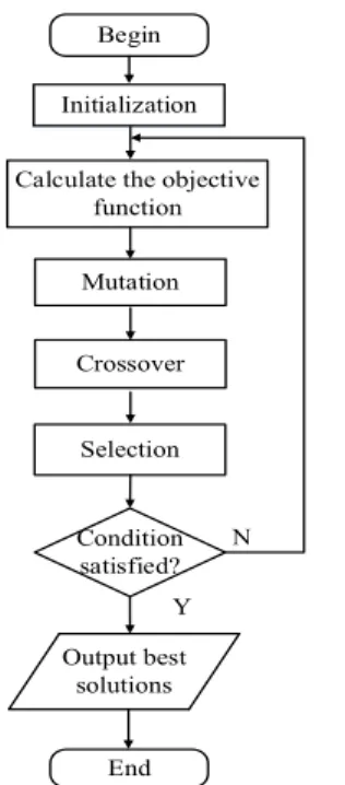
Condition satisfied?
Y N Mutation Calculate the objective
function Crossover Selection Output best solutions End Begin Initialization
Fig. 2. The flowchart of self-organizing strategy based on DE.
4) Selection: After crossover, g p
o is compared with g p
z in terms of the objective function values. The selection operation is formulated as
1 , if (F( ) F( )) , otherwise. g g g p p p g p g p + = ≤ o o z z z (19)
After the selection operation, it is known that either g p
o or g p
z survives to the next generation. 5) Stopping criterion: If the maximum generation gmax is reached, the algorithm will be terminated,
and the global best individual is acquired. Otherwise, the algorithm continues to next generation. The flowchart of the self-organizing strategy based on DE is shown in Fig. 2.
3.2 Sparse selection
It is well known that the Lagrangian multipliers play a key role in SVMs since many αi values in SVMs are equal to zero. However, compared with standard SVMs, LSSVMs lack sparseness, which is ineffective on large-scale datasets, although it is a successful variant of SVMs for transforming a series of inequality constraints to linear equations. Due to optimality conditions and αi =γei, all of the
training samples are considered as support vectors (SVs) for LSSVMs. In order to reduce computation cost and memory space, according to previous studies [25, 26], in this study, a sparse selection strategy was designed based on pruning to reduce the number of training samples. First, the αi values are
sorted to evaluate which sample contributes most to the LSSVM model. Based on the sorted αi
values of LSSVM, the sparse condition is described as follows:
i
α ≤β (20) where β is designed as a sparsity threshold value. Using Eq. (20), the less important data (corresponding to small αi ) are omitted from the training dataset.
Fig. 3 shows the physical meaning of pruning. With respect to the sorted αi spectrum, the most
significant samples are maintained in the training dataset, and the samples with least information are gradually omitted from the training dataset. This sparsity strategy does not require the information of a Hessian matrix or its inverse. Afterwards, the model of DE-MKLSSVM is re-estimated based on the
updated training dataset. To guarantee the accuracy of sparse approximation, DE is used to optimize the model parameters in each sparse process.
The sparse selection operation is carried out as follows: Step 1. The original training dataset with N samples is given.
Step 2. DE-MKLSSVM is trained, and the model parameters are obtained. Step 3.αi values are sorted in a descending order.
Step 4. If the spectrum values αi are less than β, the training samples corresponding to small αi
are removed.
Step 5. The model is retrained with the updated training dataset (N′ <N).
Step 6. Return to step 3 until the current generation number g reaches the given generation number λ. The pseudo-code of the sparse selection strategy is given in Algorithm 1 below. It should be noted that β has a great influence on the selection of training samples. If β is set to a small value, the sparsity of the training dataset will be weak. On the contrary, if β is considered as a large value, the useful samples will be omitted. Therefore, β should be chosen carefully to strike a balance between sparsity and model accuracy. Because the omitted samples have little influence on the prediction model, they may be redundant samples or outliers. Training on these samples will lead to an ill-posed problem, and have a bad effect on the model performance.
3.3 SDE-MKLSSVM
In this paper, MK learning is used to improve the prediction accuracy. The appropriate kernel functions are selected by a self-organizing strategy based on DE. Meanwhile, the corresponding kernel parameters and combination coefficients are adaptively adjusted by DE as well. Moreover, to reduce the computation cost, a sparse selection strategy is used to simplify the training dataset. A part of training samples will be omitted according to the sparsity criterion. Fig. 4 describes the schematic diagram of proposed model, and its pseudo-code is presented in Algorithm 2.
3.4 Computation complexity analysis of SDE-MKLSSVM
In the section, a computation complexity analysis of SDE-MKLSSVM is carried out. For DE-MKLSSVM, it is notable that the complexity of MKLSSVM is O(N2 d), and the complexity of DE
is O(gmax NP D), where N denotes the number of the training samples, d denotes the dimension of one
training sample, and D denotes the number of parameters to be optimized. It can be observed that gmax,
N, d, NP and D have a strong effect on self-organizing MK learning. In SDE-MKLSSVM, the number of the final training dataset N′ is much smaller than N. Thus, it can be concluded that the computation complexity of SDE-MKLSSVM is lower than that of DE-MKLSSVM.
Sparse LSSVM LSSVM N i α Sorted Training size
Algorithm 1 Sparse selection strategy 1: Given the training dataset
: ( , )
{
}
N1i
y
i i=Γ
x
, the sparsity threshold value β, and the maximum sparse selection generation number λ (stopping criterion).2. Initialize g = 0.
3:While
g
<
λ
do4: Train DE-MKLSSVM on the current training dataset Γ, and then obtain the Lagrangian multipliers αi.
5: Sort the Lagrangian multipliersαi .
6: Make the set of selected samples
Ψ
as null, and N′ =0. 7: Fori = 1 : N If αi ≤β Omit( , )
x
iy
i ; ElseΨ ←
( , )
x
iy
i ; N′++; End if End for 8: N N= ′;9: Update the training dataset
= : ( , )
{
}
N1 iy
i i′ =
Γ Ψ
x
.End while
10: Obtain the final training dataset.
Algorithm 2 SDE-MKLSSVM 1: Preprocess the original data.
2: Initialize the whole parameters of the proposed method. 3: While
g
<
λ
do4: Update training dataset by sparse selection strategy. End while
5: Obtain the final training dataset. 6: While g≥λ and
g g
<
max do7: Utilize DE to select appropriate kernel functions and optimize the corresponding parameters on the final training dataset.
End while
8: Obtain the model with best parameters. 9: Test the model.
Y N Data preprocessing
Original data
Select training samples by sparse selection strategy
Y N Optimize the model
by DE Obtain the final training
dataset
Obtain the model with best parameters Data preprocessing
Initialization
Test the model
Fig. 4. Schematic of the proposed method.
4 Experiments
To demonstrate the effectiveness of the proposed SDE-MKLSSVM, we compare it with some other state-of-the-art black-box methods on UCI benchmark datasets. To further illustrate the applicability of the proposed method, the experiment was conducted on a real-world steelmaking problem, and discussions about prediction results are presented.
4.1 Experimental setting
1) Experimental platform: The experiments are conducted on a computer with a Microsoft Windows 7 operating system, Intel® Core™ i7-6700 CPU, Microsoft Visual Studio 2008 software. The programming language is C++.
2) Parameters setting: The parameters of SDE-MKLSSVM are set in Table 1. For the black-box benchmark problems, each model was run 20 times to avoid the randomness of experimental results. For the practical application problem, to verify the generalization ability of the proposed method, SDE-MKLSSVM was tested by a 10-fold cross-validation.
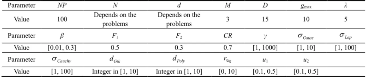
Table 1 Parameters setting of SDE-MKLSSVM.
Parameter NP N d M D gmax λ
Value 100 Depends on the problems Depends on the problems 3 15 10 5 Parameter β F1 F2 CR γ σGauss σLap
Value [0.01, 0.3] 0.5 0.3 0.7 [1, 1000] [1, 10] [1, 100] Parameter σCauchy dGtk dPoly rSig u1 u2
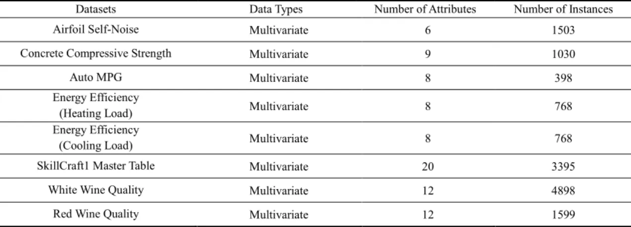
Table 2 Datasets in the UCI repository.
Datasets Data Types Number of Attributes Number of Instances Airfoil Self-Noise Multivariate 6 1503 Concrete Compressive Strength Multivariate 9 1030 Auto MPG Multivariate 8 398 Energy Efficiency
(Heating Load) Multivariate 8 768 Energy Efficiency
(Cooling Load) Multivariate 8 768 SkillCraft1 Master Table Multivariate 20 3395
White Wine Quality Multivariate 12 4898 Red Wine Quality Multivariate 12 1599
4.2 Benchmark problems in UCI repository
To analyze the characteristics of SDE-MKLSSVM, several regression problems from the UCI machine learning repository [42] are considered as black-box benchmark problems. After normalization and standardization, these data are used to verify the effectiveness of SDE-MKLSSVM and other state-of-the-art methods.
1) Experimental data: Eight datasets were chosen from the UCI repository to conduct the experiments, all having multiple attributesand with size varying from hundreds to thousands of instances. The details are given in Table 2.
2) Strategies comparison: The method proposed in this paper contains two main parts: the self-organizing MK learning strategy and the sparse selection strategy. Considering the effectiveness of different strategies, SDE-MKLSSVM is compared with DE-LSSVM and DE-MKLSSVM. Specifically, DE-LSSVM represents LSSVM with Gaussian kernel optimized by DE, and DE-MKLSSVM represents LSSVM with MK optimized by DE. Besides, SDE-MKLSSVM is compared with other LSSVM-based methods such as sparse LSSVM [43] with DE (SDE-LSSVM), and MK learning [44] based on LSSVM (MKL-LSSVM). In Table 3, four quantitative criteria are provided—root mean square error (RMSE),
mean absolute error (MAE), standard error (STDE) of the absolute prediction errors, and maximum absolute error (MAXAE). The values in bold are the best results in the comparisons. From the obtained results, it was observed that DE-LSSVM and SDE-LSSVM perform worse than MKLSSVM-based methods. This indicates the effectiveness of MK learning. In addition, SDE-MKLSSVM and DE-MKLSSVM show higher accuracy than MKL-LSSVM, demonstrating that the DE algorithm contributes to the model accuracy.
In terms of sparsity, β is set to 0.2 for all benchmark testing problems. Table 4 provides some statistic results on the reduction percentage of training samples. Compared with DE-MKLSSVM, SDE-MKLSSVM reduces the average for approximately 18% of training samples in terms of different benchmark datasets, with the computation complexity reduced to a great extent. Based on the above results, it can be seen that the proposed SDE-MKLSSVM achieves a higher accuracy than LSSVM with a single kernel and runs faster than non-sparsity methods. Therefore, SDE-MKLSSVM is suitable for black-box modeling.
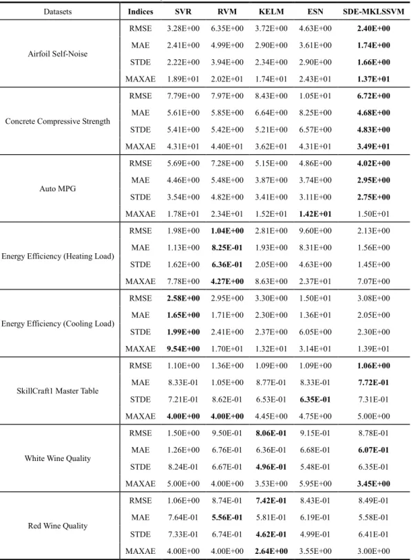
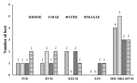
3) Comparison with state-of-the-art methods: Experiments were also conducted with other state-of-the-art methods, SVR [45], RVM [46], KELM [47] and ESN [48], to illustrate the effectiveness of the SDE-MKLSSVM. The comparison results are presented in Table 5. Besides, Fig. 5 shows the number of best results produced by SDE-MKLSSVM and the other methods. From Table 5 and Fig. 5, it can be seen that SDE-MKLSSVM is superior to other methods and presents powerful generalization ability on different benchmark problems. Specifically, SVR has a powerful regression capability for
overfits. The main reason is that SVR has a single kernel function and presents no sparsity. However, the problem can be solved by a self-organizing MK learning strategy and a sparsity strategy. The optimal combination of kernel functions is selected from various types of kernel functions, and the corresponding parameters of the model are adaptively adjusted to fit the data. Furthermore, the redundant training samples are removed by pruning. Therefore, the generalization ability of the proposed model is improved.
Table 3 Performance comparisons of SDE-MKLSSVM and other LSSVM-based methods on UCI datasets.
Datasets Indices DE-LSSVM DE-MKLSSVM SDE-MKLSSVM SDE-LSSVM MKL-LSSVM
Airfoil Self-Noise
RMSE 3.16E+00 2.34E+00 2.40E+00 3.32E+00 3.15E+00 MAE 2.36E+00 1.69E+00 1.74E+00 2.49E+00 2.35E+00 STDE 2.11E+00 1.62E+00 1.66E+00 2.19E+00 2.10E+00 MAXAE 1.69E+01 1.35E+01 1.37E+01 1.76E+01 1.69E+01 Concrete Compressive
Strength
RMSE 7.47E+00 6.69E+00 6.72E+00 7.19E+00 7.96E+00 MAE 4.94E+00 4.62E+00 4.68E+00 4.87E+00 5.92E+00 STDE 5.61E+00 4.84E+00 4.83E+00 5.29E+00 5.30E+00 MAXAE 4.90E+01 3.57E+01 3.49E+01 3.95E+01 3.93E+01
Auto MPG
RMSE 5.43E+00 4.09E+00 4.02E+00 4.96E+00 4.43E+00 MAE 4.19E+00 3.02E+00 2.95E+00 3.70E+00 3.18E+00 STDE 3.46E+00 2.77E+00 2.75E+00 3.32E+00 3.10E+00 MAXAE 1.80E+01 1.48E+01 1.50E+01 1.70E+01 1.51E+01 Energy Efficiency
(Heating Load)
RMSE 5.67E+00 2.09E+00 2.13E+00 5.33E+00 3.15E+00 MAE 4.88E+00 1.51E+00 1.56E+00 4.59E+00 2.38E+00 STDE 2.89E+00 1.45E+00 1.45E+00 2.71E+00 2.06E+00 MAXAE 1.30E+01 6.96E+00 7.07E+00 1.21E+01 9.63E+00 Energy Efficiency
(Cooling Load)
RMSE 6.84E+00 3.06E+00 3.08E+00 6.23E+00 3.37E+00 MAE 5.59E+00 2.02E+00 2.05E+00 5.00E+00 2.40E+00 STDE 3.95E+00 2.30E+00 2.30E+00 3.70E+00 2.36E+00 MAXAE 2.24E+01 1.37E+01 1.39E+01 2.08E+01 1.21E+01 SkillCraft1 Master
Table
RMSE 1.52E+00 1.07E+00 1.06E+00 1.37E+00 1.12E+00 MAE 1.11E+00 7.79E-01 7.72E-01 9.99E-01 8.35E-01 STDE 1.03E+00 7.38E-01 7.31E-01 9.34E-01 7.48E-01 MAXAE 9.65E+00 5.00E+00 5.00E+00 6.90E+00 4.45E+00
White Wine Quality
RMSE 1.05E+00 8.82E-01 8.78E-01 9.91E-01 9.13E-01 MAE 7.29E-01 6.10E-01 6.07E-01 6.90E-01 6.33E-01 STDE 7.51E-01 6.37E-01 6.35E-01 7.12E-01 6.57E-01 MAXAE 7.00E+00 3.60E+00 3.45E+00 6.35E+00 5.10E+00
Red Wine Quality
RMSE 1.17E+00 8.49E-01 8.49E-01 1.06E+00 7.90E-01 MAE 7.98E-01 5.55E-01 5.58E-01 7.15E-01 5.17E-01 STDE 8.54E-01 6.42E-01 6.41E-01 7.84E-01 5.98E-01 MAXAE 4.55E+00 3.00E+00 3.00E+00 4.10E+00 3.30E+00
Table 4 Average reduction percentage of training samples on UCI datasets. Datasets Airfoil Self-Noise Concrete Compressive Strength Energy Efficiency
(Heating Load) White Wine Quality Reduction percentage (%) 1.06E+01 1.63E+01 3.50E+01 8.25E+00
Datasets Auto MPG SkillCraft1 Master Table
Energy Efficiency
(Cooling Load) Red Wine Quality Reduction percentage (%) 1.75E+01 9.80E+00 2.95E+01 1.30E+01
Table 5 Performance comparisons of the state-of-the-art methods on UCI datasets.
Datasets Indices SVR RVM KELM ESN SDE-MKLSSVM
Airfoil Self-Noise
RMSE 3.28E+00 6.35E+00 3.72E+00 4.63E+00 2.40E+00 MAE 2.41E+00 4.99E+00 2.90E+00 3.61E+00 1.74E+00 STDE 2.22E+00 3.94E+00 2.34E+00 2.90E+00 1.66E+00 MAXAE 1.89E+01 2.02E+01 1.74E+01 2.43E+01 1.37E+01
Concrete Compressive Strength
RMSE 7.79E+00 7.97E+00 8.43E+00 1.05E+01 6.72E+00 MAE 5.61E+00 5.85E+00 6.64E+00 8.25E+00 4.68E+00 STDE 5.41E+00 5.42E+00 5.21E+00 6.57E+00 4.83E+00 MAXAE 4.31E+01 4.40E+01 3.62E+01 4.31E+01 3.49E+01
Auto MPG
RMSE 5.69E+00 7.28E+00 5.15E+00 4.86E+00 4.02E+00 MAE 4.46E+00 5.48E+00 3.87E+00 3.74E+00 2.95E+00 STDE 3.54E+00 4.82E+00 3.41E+00 3.11E+00 2.75E+00 MAXAE 1.78E+01 2.34E+01 1.52E+01 1.42E+01 1.50E+01
Energy Efficiency (Heating Load)
RMSE 1.98E+00 1.04E+00 2.81E+00 9.60E+00 2.13E+00 MAE 1.13E+00 8.25E-01 1.93E+00 8.31E+00 1.56E+00 STDE 1.62E+00 6.36E-01 2.05E+00 4.63E+00 1.45E+00 MAXAE 7.78E+00 4.27E+00 8.63E+00 2.37E+01 7.07E+00
Energy Efficiency (Cooling Load)
RMSE 2.58E+00 2.95E+00 3.30E+00 1.50E+01 3.08E+00 MAE 1.65E+00 1.71E+00 2.30E+00 1.36E+01 2.05E+00 STDE 1.99E+00 2.41E+00 2.37E+00 6.05E+00 2.30E+00 MAXAE 9.54E+00 1.70E+01 1.32E+01 3.14E+01 1.39E+01
SkillCraft1 Master Table
RMSE 1.10E+00 1.36E+00 1.09E+00 1.09E+00 1.06E+00 MAE 8.33E-01 1.05E+00 8.77E-01 8.33E-01 7.72E-01 STDE 7.21E-01 8.62E-01 6.53E-01 6.35E-01 7.31E-01 MAXAE 4.00E+00 4.00E+00 4.45E+00 4.75E+00 5.00E+00
White Wine Quality
RMSE 1.50E+00 9.50E-01 8.06E-01 9.15E-01 8.78E-01 MAE 1.26E+00 6.76E-01 6.36E-01 6.68E-01 6.07E-01 STDE 8.24E-01 6.67E-01 4.96E-01 5.48E-01 6.35E-01 MAXAE 5.00E+00 4.00E+00 3.53E+00 5.95E+00 3.45E+00
Red Wine Quality
RMSE 1.06E+00 8.74E-01 7.42E-01 8.43E-01 8.49E-01 MAE 7.64E-01 5.56E-01 5.81E-01 6.19E-01 5.58E-01 STDE 7.33E-01 6.74E-01 4.62E-01 4.99E-01 6.41E-01 MAXAE 4.00E+00 4.00E+00 2.64E+00 3.55E+00 3.00E+00
4.3 End-point prediction problems in converter steelmaking
To investigate the practicability of SDE-MKLSSVM, an experiment was conducted on a real-world application: an endpoint predictionproblem in the converter steelmaking process. By comparison with other methods, the superiority of the proposed methodwill be demonstrated.
1) Experimental background: In the steelmaking process, converter steelmaking is a crucial link of steel production: the aim is to smelt high-quality steel comprising carbon (C), manganese (Mn), silicon (Si), sulfur (S), and phosphorus (P). The product must conform to the specified molten steel quality. Moreover, to avoid accidents such as molten steel splashing, the temperature (T) of the furnace needs to be monitored in real time. Therefore, the temperature and the molten steel quality have a very strong impact on smelting. Fig. 6 shows the schematic for the production process in converter steelmaking. Due to the limitations in current measurement instruments, it is difficult to establish mechanism models. In this section, SDE-MKLSSVM is used to deal with the endpoint prediction problems.
Fig. 5. Number of best performances of each method on UCI datasets.
Pour out molten steel from spout Impurities are oxidised on the surface Oxygen Flue gas Water-cooled oxygen lance Refractory lining Molten steel Fume hood Blowing at bottom
2) Experimental data: In the iron and steel production process, a large amount of data can be collected by multi-source sensors. Temperature in the furnace is measured by flame analyzers, and compositions in the molten steel are collected by sub-lance and throwing probes. Moreover, gas quantity is detected by gas analyzers. According to the operators’ experience, the inputs of training samples can be defined as: initial T, initial C content, initial Mn content, initial Si content, initial S content, initial P content, initial weight of steel scrap, initial weight of molten iron, height of oxygen lance, flow of oxygen, flow of flue gas, flow of carbon monoxide, flow of carbon dioxide, flow of nitrogen, flow of argon and seven types of auxiliary material, i.e., 22 variables in total. The outputs are the endpoint temperature as well as the five endpoint components—C, Mn, Si, S, and P.
There are 300 input–output pairs of data collected from a plant in one month. The data were preprocessed and clustered first. Then, some outlier points were deleted. Additionally, some missing data were complemented by means of interpolation methods. The final processed data were considered as the experimental data.
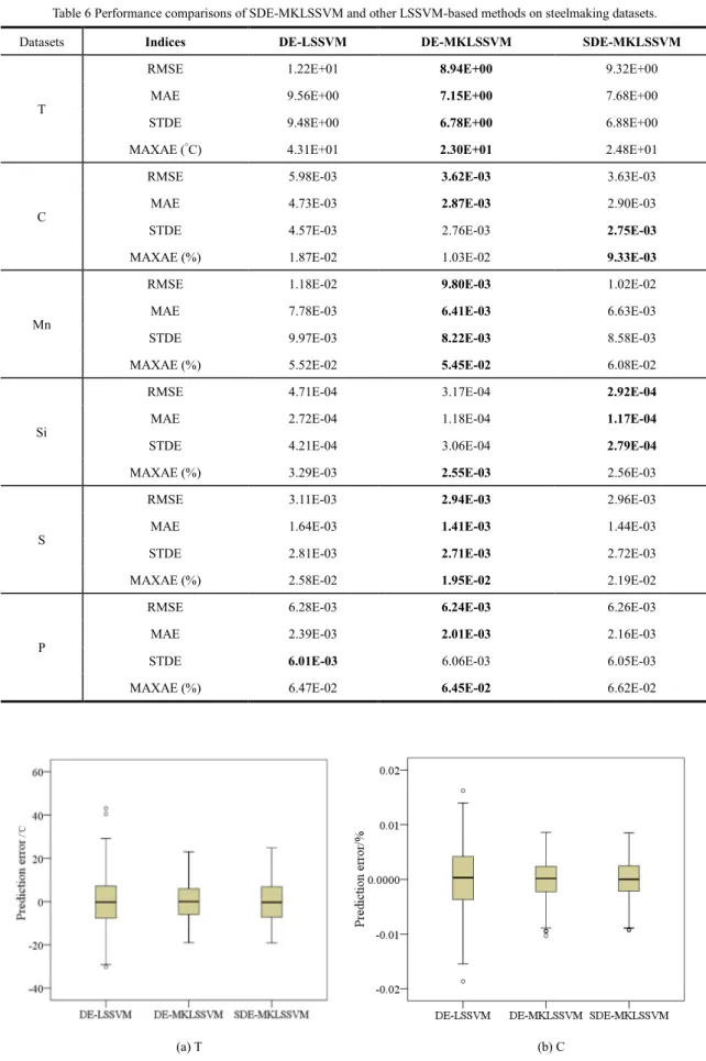
3) Experimental results: The experiment was conducted by a 10-fold cross-validation. In each cross-validation, 270 samples were used to train the model, and the remaining 30 samples were used for testing. The prediction errors of temperature and components of 300 samples produced by DE-LSSVM, DE-MKLSSVM, and SDE-MKLSSVM are shown in Fig. 7. As can be seen for SDE-MKLSSVM and DE-MKLSSVM, the absolute prediction errors of T are in the range of 0–25°C, and the absolute
prediction errors of C content are mainly in the range of 0–0.008%. Due the high temperature in the furnace, the absolute errors of Mn content are mostly between 0% and 0.02%. Owing to the desulfurization procedure, most absolute errors for S content are smaller than 0.003%. With respect to Si content and P content, the prediction errors approach to zero. Moreover, it can be observed that the absolute errors in SDE-MKLSSVM and DE-MKLSSVM are smaller than in DE-LSSVM, and there is no obvious difference in the prediction errors between DE-MKLSSVM and SDE-MKLSSVM. This means that improvements with sparsity occur with no loss of prediction accuracy.
Table 6 shows the quantitative comparison of different strategies. If the values of performance criteria are smaller than 1.0E–04, these values are regarded as zero. According to the statistic results, we can see that SDE-MKLSSVM is comparable to DE-MKLSSVM but better than DE-LSSVM, which is consistent with Fig. 7. With respect to SDE-MKLSSVM, the MAE of temperature is below 8, and the MAE of the quality component is below 0.007. This demonstrates that the prediction precision of SDE-MKLSSVM can meet actual production demand.
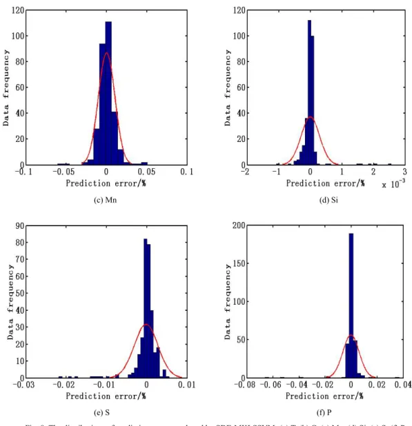
Fig.8 depicts the distributions of prediction errors produced by SDE-MKLSSVM, wherein one can clearly note that the prediction errors for all objectives conform to the normal distribution with a mean of approximately zero. As most impurities have been removed in the desulfurization and dephosphorization operations before the steelmaking process, a small quantity of Si, S, and Premains. Thus, from Fig. 8 it can be seen that there are a large number of the prediction errors around zero.
In a practical problem, the sparsity threshold value has a great influence on different models. Due to the complicated physicochemical process of reaction, there exists a relatively large range for T, and C, to balance the relationship between accuracy and complexity, the training samples should maintain adequate diversity. Thus, a small threshold value with β = 0.01 is considered in the experimental setting. For other compositions of molten steel, the change in the component contents is relatively small. Thus, a sparsity threshold of β = 0.05 is applied in the experiments. Table 7 shows the sparsity of SDE-MKLSSVM compared with DE-MKLSSVM, SDE-MKLSSVM requires 10–20% fewer training samples for predicting the T, C, and Mn contents. For other component contents (Si, S, and P), the reduction in training samples exceeds 30%.
The aforementioned results demonstrate the effectiveness of the proposed method on endpoint prediction in the converter steelmaking process. The SDE-MKLSSVM method contributes to safe
Table 6 Performance comparisons of SDE-MKLSSVM and other LSSVM-based methods on steelmaking datasets. Datasets Indices DE-LSSVM DE-MKLSSVM SDE-MKLSSVM
T
RMSE 1.22E+01 8.94E+00 9.32E+00 MAE 9.56E+00 7.15E+00 7.68E+00 STDE 9.48E+00 6.78E+00 6.88E+00 MAXAE (°C) 4.31E+01 2.30E+01 2.48E+01
C
RMSE 5.98E-03 3.62E-03 3.63E-03 MAE 4.73E-03 2.87E-03 2.90E-03 STDE 4.57E-03 2.76E-03 2.75E-03 MAXAE (%) 1.87E-02 1.03E-02 9.33E-03
Mn
RMSE 1.18E-02 9.80E-03 1.02E-02 MAE 7.78E-03 6.41E-03 6.63E-03 STDE 9.97E-03 8.22E-03 8.58E-03 MAXAE (%) 5.52E-02 5.45E-02 6.08E-02
Si
RMSE 4.71E-04 3.17E-04 2.92E-04 MAE 2.72E-04 1.18E-04 1.17E-04 STDE 4.21E-04 3.06E-04 2.79E-04 MAXAE (%) 3.29E-03 2.55E-03 2.56E-03
S
RMSE 3.11E-03 2.94E-03 2.96E-03 MAE 1.64E-03 1.41E-03 1.44E-03 STDE 2.81E-03 2.71E-03 2.72E-03 MAXAE (%) 2.58E-02 1.95E-02 2.19E-02
P
RMSE 6.28E-03 6.24E-03 6.26E-03 MAE 2.39E-03 2.01E-03 2.16E-03 STDE 6.01E-03 6.06E-03 6.05E-03 MAXAE (%) 6.47E-02 6.45E-02 6.62E-02
/
℃
(c) Mn (d) Si
(e) S (f) P Fig. 7. Boxplots of prediction errors produced by DE-LSSVM, DE-MKLSSVM and SDE-MKLSSVM: (a) T, (b) C, (c) Mn, (d) Si,
(e) S, (f) P.
(c) Mn (d) Si
(e) S (f) P
Fig. 8. The distributions of prediction errors produced by SDE-MKLSSVM: (a) T, (b) C, (c) Mn, (d) Si, (e) S, (f) P. Table 7 The average reduction percentage of training samples for the converter steelmaking process.
Datasets T C Mn Reduction percentage (%) 1.48E+01 1.07E+01 2.04E+01
Datasets Si S P Reduction percentage (%) 3.15E+01 3.33E+01 3.59E+01
5 Conclusions
This paper focuses on black-box modeling of regression problems. To solve these problems, a new framework was developed based on LSSVM with a self-organizing MK learning strategy and a sparse selection strategy (SDE-MKLSSVM). Several base kernel functions were combined to form MK learning. The optimal kernel functions and corresponding model parameters were selected by DE with an improved mutation strategy. In order to make the model efficient for large datasets, a sparse selection strategy was used to reduce the number of training samples. Numerical results on some benchmark datasets verify that SDE-MKLSSVM performs better than other state-of-the-art methods and strategies. Additionally, to further verify the practicability of the proposed method, it was used to predict the endpoint temperature and molten steel quality in the converter steelmaking process. Experimental
results sustain that SDE-MKLSSVM can meet actual production requirements over a wide range of instances.
In the processing industry, there are some problems involving dynamic process prediction instead of static endpoint prediction. These problems can be solved by multi-stage modeling. In future, it will be attempted to establish multi-stage models based on the proposed method. According to the variation between the real output and the expectation output, the operation scheme can be dynamically optimized. In addition, an attempt is made to develop dynamic multi-objective optimization algorithms to further solve the operation optimization models.
Acknowledgments. This work was supported in part by the National Key Research and Development Program of China under Grant 2016YFB0901900, in part by the Fund for Innovative Research Groups of the National Natural Science Foundation of China under Grant 71621061, in part by the National Natural Science Foundation of China through the Major International Joint Research Project under Grant 71520107004, in part by the Major Program of National Natural Science Foundation of China under Grant 71790614, in part by the 111 Project under Grant B16009, and in part by the National Natural Science Foundation of China under Grants 61702077.
References
[1] T. M. Mitchell, Machine learning, New York: McGraw-Hill, 1997.
[2] N.Y. Zeng, H. Zhang, Y.R. Li, J.L. Liang, A.M. Dobaie, Denoising and deblurring gold immunochromatographic strip images via gradient projection algorithms, Neurocomputing 247 (2017) 165–172.
[3] R. Ak, O. Fink, E. Zio, Two machine learning approaches for short-term wind speed time-series prediction, IEEE Trans. Neural Netw. Learn. Syst. 27 (8) (2016) 1734–1747.
[4] Z.W. Zhu, N. Anwer, Q. Huang, L. Mathieu, Machine learning in tolerancing for additive manufacturing, CIRP Ann. Manuf. Technol. 67 (1) (2018) 157–160.
[5] M. Khalaf, A.J. Hussain, R. Keight, D.A. Jumeily, P. Fergus, R. Keenan, P. Tso, Machine learning approaches to the application of disease modifying therapy for sickle cell using classification models, Neurocomputing 228 (2017) 154–164.
[6] T. Wuest, C. Irgens, K.D. Thoben, An approach to monitoring quality in manufacturing using supervised machine learning on product state data, J. Intell. Manuf. 25 (5) (2014) 1167–1180. [7] X. He, Z.D. Wang, Y. Liu, D.H. Zhou, Least-squares fault detection and diagnosis for networked
sensing systems using a direct state estimation approach, IEEE Trans. Ind. Inf. 9 (3) (2013) 1670–1679.
[8] C. Lian, Z.G. Zeng, W. Yao, H.M. Tang, C.L.P. Chen, Landslide displacement prediction with uncertainty based on neural networks with random hidden weights, IEEE Trans. Neural Netw. Learn. Syst. 27 (12) (2016) 2683–2695.
[9] P.R. Xu, H. Peng, T. Huang, Unsupervised learning of mixture regression models for longitudinal data, Comput. Statist. Data Anal. 125 (2018) 44–56.
[10] O. Kilinc, I. Uysal, GAR: An efficient and scalable graph-based activity regularization for semi-supervised learning, Neurocomputing 296 (2018) 46–54.
[11] M. Khanzadeh, S. Chowdhury, M. Marufuzzaman, M.A. Tschopp, L. Bian, Porosity prediction: Supervised-learning of thermal history for direct laser deposition, J. Manuf. Syst. 47 (2018) 69–82. [12] I. Chikalov, S. Hussain, M. Moshkov, Bi-criteria optimization of decision trees with applications to
data analysis, Eur. J. Oper. Res. 266 (2) (2018) 689–701.
[13] Z.D. Wang, X.H. Liu, Y.R. Liu, J.L. Liang, and V. Vinciotti, An extended Kalman filtering approach to modeling nonlinear dynamic gene regulatory networks via short gene expression time series,
[14] L. Breiman, Random forests, Machine Learning, 45 (1) (2001) 5–32.
[15] V. N. Vapnik, The nature of statistical learning theory. New York: Springer, 1995.
[16] S.M. Salaken, A. Khosravi, T. Nguyen, S. Nahavandi, Extreme learning machine based transfer learning algorithms: A survey, Neurocomputing 267 (2017) 516–524.
[17] D.H. Wang, M. Li, Stochastic configuration networks: Fundamentals and algorithms, IEEE Trans. Cybern. 47 (10) (2017) 3466–3479.
[18] N.Y. Zeng, Z.D. Wang, B. Zineddin, Y.R. Li, M. Du, L. Xiao, X. H. Liu, T. Young, Image-based quantitative analysis of gold immunochromatographic strip via cellular neural network approach, IEEE Trans. Med. Imag. 33 (5) (2014) 1129–1136.
[19] H. He, S. Chen, K. Li, X. Xu, Incremental learning from stream data, IEEE Trans. Neural Netw. 22 (12) (2011) 1901–1914.
[20] C.L.P. Chen, Z.L. Liu, Broad learning system: An effective and efficient incremental learning system without the need for deep architecture, IEEE Trans. Neural Netw. Learn. Syst. 29 (1) (2018) 10–24.
[21] W.B. Liu, Z.D. Wang, X.H. Liu, N.Y. Zeng, Y.R. Liu, F.E. Alsaadi, A survey of deep neural network architectures and their applications, Neurocomputing 234 (2017) 11–26.
[22] M.L. Xu, M. Han, Adaptive elastic echo state network for multivariate time series prediction, IEEE Trans. Cybern. 46 (10) (2016) 2173–2183.
[23] J.A.K. Suykens, J. Vandewalle, Least squares support vector machine classifiers, Neural Process. Lett. 9 (3) (1999) 293–300.
[24] S.S. Zhou, Sparse LSSVM in primal using Cholesky factorization for large-scale problems, IEEE Trans. Neural Netw. Learn. Syst. 27 (4) (2016) 783–795.
[25] R. Mall, J.A.K. Suykens, Very sparse LSSVM reductions for large-scale data, IEEE Trans. Neural Netw. Learn. Syst. 26 (5) (2015) 1086–1097.
[26] J.A.K. Suykens, L. Lukas, J. Vandewalle, Sparse approximation using least squares support vector machines, in IEEE Proc. Int. Symp. Circuits Syst. 2 (2000) 757–760.
[27] L.X. Yang, S.Y. Yang, R. Zhang, and H.H. Jin, Sparse least square support vector machine via coupled compressive pruning, Neurocomputing 131 (2014) 77–86.
[28] Y.H. Chen, M. Kloft, Y. Yang, C.H. Li, L. Li, Mixed kernel based extreme learning machine for electric load forecasting, Neurocomputing 312 (2018) 90–106.
[29] W. Chung, J. Kim, H. Lee, E. Kim, General dimensional multiple-output support vector regressions and their multiple kernel learning, IEEE Trans. Cybern. 45 (11) (2015) 2572–2584.
[30] Y.Q. Wang, X.W. Liu, Y. Dou, Q. Lv, Y. Lu, Multiple kernel learning with hybrid kernel alignment maximization, Pattern Recognit. 70 (2017) 104–111.
[31] F. Aiolli, M. Donini, EasyMKL: a scalable multiple kernel learning algorithm, Neurocomputing 169 (2015) 215–224.
[32] F. Friedrichs, C. Igel, Evolutionary tuning of multiple SVM parameters, Neurocomputing 64 (2005) 107–117.
[33] N.Y. Zeng, H. Qiu, Z.D. Wang, W.B. Liu, H. Zhang, Y.R. Li, A new switching-delayed-PSO-based optimized SVM algorithm for diagnosis of Alzheimer’s disease, Neurocomputing 320 (2018) 195–202.
[34] K.C. Lin, S.Y. Chen, J.C. Hung, Feature selection and parameter optimization of support vector machines based on modified artificial fish swarm algorithms, Math. Probl. Eng. 2015 (2015) 604108.
[35] R. Storn, K. Price, Differential evolution-a simple and efficient adaptive scheme for global optimization over continuous spaces, J. Glob. Optimiz. 11 (4) (1997) 341–359.
for global numerical optimization, IEEE Trans. Evol. Comput. 13 (2) (2009) 398–417.
[37] G.H. Wu, X. Shen, H.F. Li, H.K. Chen, A.P. Lin, P.N. Suganthan, Ensemble of differential evolution variants, Inf. Sci. 423 (2018) 172–186.
[38]C.R. Souza, Kernel functions for machine learning applications [Online], 2010, Available: http://crsouza.com/2010/03/17/kernel-functions-for-machine-learning-applications/.
[39] L.A. Belanche, A. Tosi, Averaging of kernel functions, Neurocomputing 112 (2013) 19–25.
[40] R. Kannao, P. Guha, Success based locally weighted multiple kernel combination, Pattern Recognit. 68 (2017) 38–51.
[41] S.S. Shiju, S. Asif, S. Sumitra, Multiple kernel learning using composite kernel functions, Eng. Appl. Artif. Intell. 64 (2017) 391–400.
[42] A. Frank, A. Asuncion, UCI machine learning repository [Online], 2010, Available: http://archive.ics.uci.edu/ml/.
[43] J.A.K. Suykens, J.D. Brabanter, L. Lukas, J. Vandewalle, Weighted least squares support vector machines: robustness and sparse approximation, Neurocomputing 48 (1–4) (2002) 85–105.
[44] A. Rakotomamonjy, F.R. Bach, S. Canu, Y. Grandvalet, Simple MKL, J. Mach. Learn. Res. 9 (2008) 2491–2521.
[45] H. Drucker, C. J. Burges, L. Kaufman, A. Smola, V. Vapnik, Support vector regression machines, in Advances in Neural Information Processing Systems (1997) 155–161.
[46] M.E. Tipping, Sparse Bayesian learning and the relevance vector machine, J. Mach. Learn. Res. 1 (2001) 211–244.
[47] G.B. Huang, H.G. Zhou, X.J. Ding, R. Zhang, Extreme learning machine for regression and multiclass classification, IEEE Trans. Syst., Man, Cybern. B, Cybern. 42 (2) (2012) 513–529. [48] H. Jaeger, H. Haas, Harnessing nonlinearity: Predicting chaotic systems and saving energy in