Teaching Development Project: Gene Expression Prediction With Deep Learning

(1)

PREDICTION WITH DEEP LEARNING

Master of Science thesis

Examiner: University lecturer Heikki Huttunen

Examiner and topic approved by the Faculty Council of the Faculty of Computing and Electrical Engineering on 1 February 2017

(2)

ABSTRACT

LINGYU ZHU: TEACHING DEVELOPMENT PROJECT: GENE EXPRESSION PREDICTION WITH DEEP LEARNING

Tampere University of Technology Master of Science thesis, 59 pages May 2017

Master’s Degree Programme in Information Technology Major: Data Engineering

Minor: Signal Processing

Examiner: University lecturer Heikki Huttunen

Keywords: Gene expression, histone modification, deep Learning, convolutional recurrent neural network

Histone modifications are playing an important role in aﬀecting gene regulation. In this thesis, a Convolutional Recurrent Neural Network is proposed and applied to predict gene expression levels from histone modification signals. Its two simpli-fied variants: Convolutional Neural Network and Recurrent Neural Network, and one state-of-the-art baseline: DeepChrome are also discussed in this work. Their performances are evaluated with gene expression data that derived from Roadmap Epigenomics Mapping Consortium database by the Receiver Operating Character-istic, Area Under the Curve and statistical analysis. As a result, the Convolutional Recurrent Neural Network model achieves the best performance compared to the other models.

For teaching development of a pattern recognition and machine learning course from Tampere University of Technology, an approach of integrating theory and practice is used. Video recording, weekly exercises and competition are worked as the auxiliary parts of lectures, which helps the students have a better understanding of the the-oretical knowledge and learn how to solve diﬀerent kind of practical problems. We used histone modification data for a competition on this course, and this competition would be discussed emphatically in this thesis. For the competition, we motivated the students to develop multiple machine learning algorithms to accurately predict gene expression levels on five core histone modification masks. During the period of this course, the competition Gene Expression Prediction received 888 entries that submitted by 105 teams with 184 players. This thesis includes the analysis and sum-mary of the outcomes from the competition. Additionally, the learning assessment is also discussed in this thesis.

(3)

PREFACE

With the rapid development of biotechnology and the advent of microarrays, there is an enormous explosion of biological data. This massive data has made the con-ventional analysis methods face a tremendous challenge. Diﬀerent machine learning methods have draw attention from people due to their state-of-the-art performance in this field, especially deep learning. Our goal in this work is to predict gene ex-pression levels with deep learning, and we choseGene Expression Prediction as the topic of competition which is a practical auxiliary extension of a pattern recognition and machine learning course from Tampere University of Technology. This compe-tition was jointly organized by Tampere University of Technology and University of Tampere. Most of the participants are the students from those two universities, they have diﬀerent backgrounds: information technology and computing biology. The students could obtain both of the theoretical knowledge and practical skills from this course if they attend all of the ”activities” that this course involved. The analysis between the design of the course from faculty and the feedback from the competition participants makes an excellent closed loop of reference for the future development of this course.

I would like to express my deep gratitude to my supervisor Heikki Huttunen for excellent guidance, reviewing the manuscript, and giving constructive comments of my thesis during this project. I also warmly thank Professor Matti Nykter and Juha Kesseli who have always being willing to providing support and insightful suggestions whenever needed. Moreover, I wish to thank all my coworkers for their contribution to this Gene Expression Prediction competition, and my warm thanks are extended to all the competition participants for their enthusiasm and invaluable feedback.

Finally, I would like to appreciate the valuable encouragement and support from my kind parents and all warm friends.

Lingyu Zhu 22 May, 2017

(4)

LIST OF FIGURES

2.1 Mapping input to output. . . 5

2.2 Simple linear regression solutions. . . 6

2.3 KNN of the unseen observation. . . 9

2.4 Multiple solutions of SVM. . . 10

2.5 Decision boundary of SVM. . . 11

2.6 Random forest. . . 12

2.7 Tree ensemble model (age and male), adapted from [31]. . . 14

2.8 Tree ensemble model (use computer daily), adapted from [31]. . . 15

2.9 A simple biological neuron network. . . 16

2.10 A feedforward neural network model. . . 17

2.11 Architecture of Convolutional Neural Network (adapted from [37]). . 19

2.12 Three dimensional volume. . . 20

2.13 Receptive fields (adapted from [38]). . . 21

2.14 Maxpooling (adapted from [34]). . . 22

2.15 A recurrent neural network with unfolding in time (adapted from [39]). 23 2.16 Examples of Recurrent Neural Network sequential model (adapted from [40]). . . 24

2.17 Illustration of (a) LSTM and (b) GRU. (adapted from [41]) . . . 25

3.1 Architecture of CRNN model(adapted from [17]). . . 30

3.2 Architecture of CNN model(adapted from [17]). . . 31

(7)

3.4 Architecture of DeepChrome model used in this work(adapted from [17]). 32

4.1 Confusion matrix. . . 35

4.2 Distribution of predicted probabilities. . . 36

4.3 ROC curve for the first distribution example. . . 36

4.4 ROC curve for the second distribution example. . . 37

4.5 ROC curve for the third distribution example. . . 37

4.6 Comparison of ROC curves. . . 38

4.7 P-value. . . 39

4.8 AUC scores over 56 cell types. . . 42

4.9 The ROC curves of studied models of cell type ”E065”. . . 43

4.10 The ROC curves of cell type ”E047” from top 5 submissions, CRNN model and KNN benchmark. . . 48

(8)

LIST OF TABLES

3.1 Five core histone modification marks. . . 28

4.1 Performance of studied models on test dataset. (adapted from [17]) . 42 4.2 The weighted AUC scores from the top 5 teams, proposed CRNN

model and one benchmark. . . 45 4.3 P-values and AUC diﬀerences of cell type ”E047” from top 5

(9)

LIST OF ABBREVIATIONS

ADAM Adaptive Moment Estimation AUC Area Under the Curve

BPTT Back Propagation Through Time CART Classification and Regression Trees CNN Convolutional Neural Network

CRNN Convolutional Recurrent Neural Network

FN False Negative

FP False Positive FPR False Positive Rate GRU Gated Recurrent Unit KNN K-nearest Neighbors LR Linear Regression

LSTM Long Short Term Memory

REMC Roadmap Epigenomics Mapping Consortium ReLU Rectified Linear Unit

RF Random Forest

RNN Recurrent Neural Network

ROC Receiver Operating Characteristic SGD Stochastic Gradient Descent SVM Support Vector Machine TanH Hyperbolic Tangent

TN True Negative

TP True Positive

TPR False Positive Rate TSS Transcription Start Site

(10)

1.

INTRODUCTION

Gene expression prediction can be regulated from various gene activity stages that range from the transcription of DNA-RNA to multiple post-translational protein modifications. The wide variety of mechanisms probably will facilitate or suppress the gene expression regulation. Histone modification is one of the most essential factors that aﬀect gene expression from a transcription aspect. Histone proteins serve to wrap the DNA strands into chromosomes and select the genes that would get transcribed in cells. [1], [2].

The gene expression levels can be modeled and predicted using different machine learning algorithms. Machine learning is a data analysis method that enables com-puters to have the ability of model building and learning automatically. It helps computers to do pattern recognition and to find hidden insights without being pro-grammed explicitly. In comparison to the conventional biological computational methods, machine learning has been put into practice with the research on studying the correlation of gene expression and histone modifications in many attempts [3]. For instance, quantitative models [4], Support Vector Machine (SVM) model [5] and Random Forest (RF) Classifier model [6] have been proposed to correlate the gene regulation with histone modification signals. As the averaging methods that pre-vious studies used for capturing the input features from gene transcription region leave out some important details [4], and predicting separately for different feature regions using multiple models will seriously affect the final prediction accuracy. To avoid these problems, a deep learning method on this topic was proposed recently in [7].

Deep learning is a branch of machine learning with more complicated algorithms which can model features with high level abstraction from data. It has achieved the state-of-the-art performance in several fields such as image classification [8], [9], [10], semantic segmentation [11] and speech recognition [12], [13]. Recently, deep learning methods have also achieved success in computational biology [7], [14], [15]. There-fore, diﬀerent machine learning methods, especially deep learning, have started be-ing applied on this work for predictbe-ing gene expression levels from five core histone modifications [16]. In this thesis, we study how the Convolutional Recurrent Neural

(11)

Network (CRNN) performs for predicting the gene regulation tasks and compare its performance to Convolutional Neural Network (CNN), Recurrent Neural Network (RNN) and a convolutional baseline: DeepChrome [7]. Additionally, this work was accepted as a conference paper [17] on 11 April, 2017.

We used the gene activity prediction as an example case for a teaching experiment, and one machine learning competitionGene Expression Prediction was jointly orga-nized by Tampere University of Technology and University of Tampere. Its outcome and feedback from the participants will also be discussed in this thesis.

The remainder of this thesis is arranged as follows. In Chapter 2, the theoreti-cal background is presented, it includes machine learning, neural networks, deep learning backgrounds and the existing computational methods of predicting gene expression levels. Chapter 3 introduces data and the architecture of the proposed models. In Chapter 4, the performance of the studied models is evaluated. Ad-ditionally, the result of the Gene Expression Prediction competition and learning assessment is also presented in Chapter 4. Finally, conclusions and possible future work are discussed in Chapter 5.

(12)

2.

THEORETICAL BACKGROUND

2.1

Machine Learning

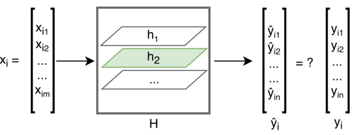
The definition of machine learning: ”A computer program is said to learn from experience E with respect to some class of tasks T and performance measure P if its performance at tasks inT, as measured by P, improves with experience E” that proposed by Tom Mitchell in [18] is widely quoted. The working principle of machine learning is building a data driven model which can produce reliable predictions based on the computations in the training process. It can be applied in many fields, for example, financial services, health care, marketing and sales, transportation and so on. In this thesis, it is a binary classification task with biological genomic data. The ultimate goal is to learn and select a hypothesis h, which minimizes the differences between predictions yˆ_i = (ˆyi1,yî2, . . . ,yîn) and desired labels yi = (yi1, yi2, . . . , yin)

of input xi = (xi1, xi2, . . . , xim), from a class of hypotheses H and accurate predict

gene expression levels. The i corresponds to the i-th instance that ranges from 1 toN, where N is the number of total instances. The m and n represent the input and output dimensions of each instance, respectively. Moreover, machine learning algorithms are typically distinguished into the following three categories: supervised learning, unsupervised learning and semi-supervised learning, depending on the data available and the purpose of diﬀerent tasks.

Supervised learning: Supervised learning is where the target labels are known and you try to figure out one hypothesis h from hypotheses set H that can map the input xi to output yi, which is illustrated in Figure 2.1. The supervised learning

algorithms iteratively make predictions on labeled examples and are corrected by minimizing the errors between the predictions yˆ_i and the known desired labels y_i. Supervised learning can be further grouped into two subcategories: regression and classification. The regression is used to model the correlation between input samples and targets which are continuous while the targets of classification are categorical. Depending on the diﬀerent tasks, various supervised learning algorithms can be applied, such as Linear Regression (LR), K-nearest Neighbors (KNN), SVM, decision trees, RF and so on. [19], [20]

(13)

Figure 2.1 Mapping input to output.

Unsupervised learning: Unsupervised learning refers to the cases that the data has no target labels. The goal of the unsupervised learning algorithms is to find out the hidden structure within the data. They are called unsupervised learning be-cause the ”right answer” is unknown and there is no ”supervisor” here for super-vising the learning process. The unsupervised learning can be also grouped into two subcategories: clustering and association. Clustering, such as k-means [21] and self-organizing maps [22], [23], helps us to discover the inherent property within the data while the association rule learning algorithms, like Apriori [24], discover the rules that represent the large portion of data.

Semi-supervised learning: Semi-supervised learning sits in between supervised learn-ing and unsupervised learnlearn-ing, it involves the function estimation on labeled and unlabeled data. The proposal of this modeling method is motivated by the fact that the cost associated with labeling data is usually high, whereas the unlabeled data is relatively cheap and easy to collect. Semi-supervised learning uses both labeled and unlabeled data for training, typically a large amount of unlabeled data with a small amount of labeled data. A mixture of supervised and unsupervised learning techniques can be used in this concept. [25], [26]

As the task in this thesis is a supervised learning problem, few machine learning algorithms related to supervised learning such as LR, KNN, SVM, RF, and XGBoost are introduced in this section.

2.1.1

Linear Regression

LR is the very basic predictive analysis for regression problems. Several linear regression analyses are commonly studied such as simple linear regression, logistic regression, multiple linear regression, ordinal regression, multinominal regression

(14)

and discriminant analysis. For visualization purpose, the concept and basic principle of simple linear regression is particularly discussed.

As the linear regression, in this case, concerns only the study of one independent variable, people named it as simple linear regression. It is an elementary and statis-tical method that enables us to figure out the statisstatis-tical relationships between two quantitative variables. One variable is usually called the explanatory or independent variable and refereed asxi here. Another variable, referred as yi, is regarded as the

response or dependent variable. In simple linear regression, we try to form and draw a straight line with the prediction ˆyi which are mapped as:

ˆ

yi =axi+b (2.1)

where the parametersa and b are constants, and represent the slope and intercept of the final optimal regression line, respectively. i is the i-th instance of total N samples. The goal is to find the best fitting straight line, usually called regression line, through all data points.

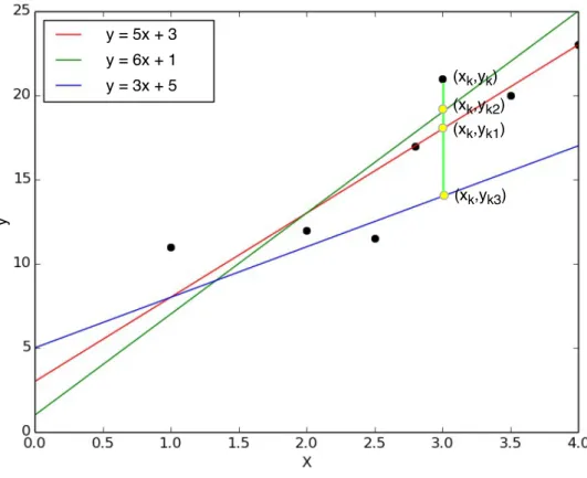
Figure 2.2 Simple linear regression solutions.

(15)

2.2 consists of six black points and three straight lines. The six black dots have their corresponding independent variable valuesxi and desired dependent variable values

yi. The three straight lines consist of the predicted values ˆyi for each possible value

of xi. The three dots that are marked as yellow represent the predicted values on

one samexk, where thekmeans the k-th instance. The top black point corresponds

to the desired dependent variable value yk on this xk. The distance between each

yellow dot and the black one on the samexk is called as prediction error. As we can

see, the yellow point (xk, yk2) on the green line is near the black point (xk, yk) most.

By contrast, the distance between the yellow point (xk, yk3) on the blue straight

line and that black dot is much larger than the others and therefore its prediction error of this ”blue solution” is the largest one on this independent variable value xk. By summing the squared prediction errors of all data points with each of the

three straight lines in Figure 2.2, we conclude that the red line is the best fitting line in this case as it has the minimum squared errors. The best fitting line is defined as the regression line that minimizes the sum of the squared errors of prediction. Accordingly, we could obtain the parametersaandbwhich minimize the total errors E in Equation 2.2 and Equation 2.3:

E = N ∑ i=1 (yi−yˆi) (2.2) E = N ∑ i=1 (yi −(axi +b)) (2.3)

2.1.2

K-nearest Neighbors

KNN is a widely and commonly used classification technique because of its easy interpretation and low calculation time, and it is also often applied as a benchmark for the other models. KNN belongs to one member of the family of lazy learning, instance-based and competitive learning algorithms. Lazy learning is a learning method that only builds a model completely until the time when a prediction is required. In other words, the KNN algorithm is such a lazy learning method only does work at the last second. KNN algorithm also belongs to the instance-based algorithms as it models problems with all the training observations in order to make an accurate predictive decision. Moreover, as a competitive learning algorithm, KNN internally involves competition between data instances of model in order to make a predictive decision. The measurement of objective similarity, such as majority vote, among the data instances causes each data sample to compete to ”win” and contribute to a prediction.

(16)

KNN is based on the idea of predicting unknown samples by comparing them with the most similar known values. Let us assume that we have two diﬀerent types of data points in Figure 2.3. A spread of red circles and green squares belong to diﬀerent classes. Our task is to find out which category the blue triangle belongs to. In the classification setting of KNN, theKindicates the number of nearest neighbors that we will consider when giving a new unseen data. The KNN algorithm will form a majority vote among theK most similar neighbors to this given unseen observation (x01, x02). The similarity is defined based on the distance metric among the two sets

of data points. A common way to calculate the distance is the Euclidean distance which is formulated as:

DEuclidean =

√

(x1−x01)2 + (x2−x02)2 (2.4)

where (x1, x2) corresponds to the coordinates of the points in Figure 2.3 and the

(x01, x02) represents the unseen data point that needs prediction. Additionally, the

Chebyshev and Manhattan distance are also often considered for calculating the distance metric [27]. Chebyshev distance is defined as the largest distance along all the coordinate dimension of two vectors. Manhattan distance sum the distances between two points measured along all axes. They are defined as below:

DChebyshev= max(|x1−x01|,|x2−x02|) (2.5)

DM anhattan=|x1 −x01|+|x2 −x02| (2.6)

The KNN runs through the whole dataset and computes the distanceDbetween this unseen observation (x01, x02) and each training data. If the given positive integerK

is 3, a 3 nearest neighbors area is shown in Figure 2.3. KNN then takes a majority vote among the points within this area. As we can see, among the three closest points to this blue triangle, two of them are the red circles and one is the green square. It is obvious that the observed blue triangle belongs to the red circle class with the K = 3. However, for the 7 nearest neighbors when theK = 7, 4 of them are the green squares which are more than the number of red circles. Therefore, this blue triangle gets assigned to the class with the largest probability (4₇). The choice of the parameter K is very crucial in this algorithm. We need to conclude an optimal K in order to get the best possible fit for the dataset. A higher K averages more voters in each prediction and hence is more resilient to outliers. Larger values of K will give smoother decision boundaries which means lower variance but increased bias. A smallK gives a more flexible fit with higher variance but low bias. Besides, the value ofK that we choose is usually odd to prevent the tie situations in a binary classification case.

(17)

Figure 2.3 KNN of the unseen observation.

2.1.3

Support Vector Machine

SVM is a supervised machine learning algorithm which can be applied for both the regression and classification challenges, and it is mostly used for classification tasks. When solving a classification problem, the SVM is a discriminative classifier which will output an optimal hyperplane. This hyperplane is capable of categorizing new examples well.

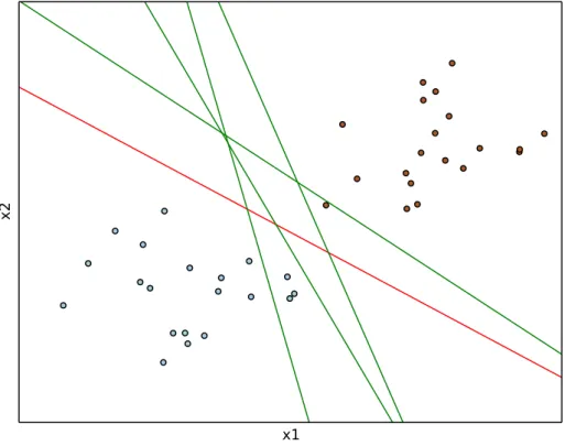
In this example, a linearly separable set of 2 dimensional points which belong to one of two classes are discussed. The 2 dimension here corresponds to the number of at-tributes that locate their values on a particular coordinate. If we had three features, we could have a 3 dimensional graph. The goal is to figure out an optimal separating straight line in this example. We deal with the data points and hypothetical lines in the Cartesian plane instead of hyperplanes in a high dimensional space for problem visualization and simplification. However, the same working concept can be applied to classify data points in a higher dimension space.

In Figure 2.4, there exists several possible solutions to the problem. The operation of the SVM algorithm is aim to find the best separating hyperplane that mostly widen

(18)

x1

x2

Figure 2.4 Multiple solutions of SVM.

the margin of the training dataset. The training process involves the minimization of the error function:

E = 1 2w T_w₊_C N ∑ i=1 ξi (2.7)

subject to the constraints:

y_i (

wTϕ(xi) +b

)

≥1−ξi (2.8)

where w is the coeﬃcients vector, b is a bias, C is the capacity constant, and the larger the C the larger error is penalized. ξi ≥ 0 represents the parameters of

dealing with the non-separable inputs. xi symbolizes the training examples while

the y_i(+1,−1) represents the class labels. The kernel ϕ represents the operation that used to transform data points from the input to the feature space. [28] Finally, the problem of minimizing the error function E is equivalent to the maximization of margins. The red straight line in Figure 2.4 is the optimal decision boundary, among the available choices, that classifies the classes accurately and maximizing the margins also. This separating hyperplane and the margins are illustrated in Figure 2.5. In general, the samples that are closest to the hyperplane are called

(19)

support vectors. The support vectors are marked with yellow circles and plotted around the black dash lines (margins) in Figure 2.5.

x1

x2

Figure 2.5 Decision boundary of SVM.

It is easy to visualize and have a linear hyperplane for the 2 dimensional data in this example. However, not every dataset is linearly separable. SVM has a technique called thekernel trick which can transform the feature vector xi with the nonlinear

mapping operation ϕ in Equation 2.8 into a higher dimensional space and convert the not separable problem to separable one. [28]

2.1.4

Random Forest

RF is based on a bagging technique with the idea that the combination of learning models can improve the classification accuracy significantly. Bagging averages the unbiased and noisy models and creates a new model with a lower variance. RF works as a large collection of uncorrelated decision trees and uses them to make a classification. In a decision tree, instances are entered at the roof and as they traverse down the tree the instances get bucketed into smaller and smaller subsets.

(20)

A decision tree is a straightforward divide-and-conquer diagram that combines in-dividual attributes into a decision. However, the decision tree is easy to over-learn the data, which means that the created model will memorize the training set with a poor ability to generalize. RF overcomes this by training diﬀerent ”imperfect” trees. [29]

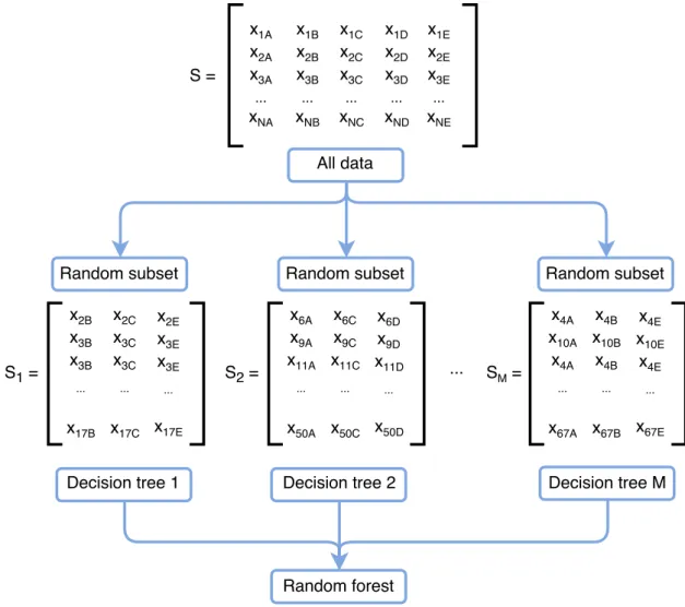
Figure 2.6 Random forest.

We suppose the matrix S in Figure 2.6 is the training set (N instances with 5 fea-tures). Each row corresponds to one instance and the columns are features. For example, thex1B is featureB of the first sample, and xN E represents the feature E

of the N-th instance. Firstly, we create random subsetsSi from the matrix S.

Em-phatically, the selection of rows is with replacement while the columns are sampled without replacement. Afterwards, we train separate decision trees based on each random subset, which is illustrated in Figure 2.6. Each decision tree executes the diﬀerent variations of the main classification task. All these decision trees constitute a forest, and create a ranking of classifiers. The RF will make the prediction by tak-ing the majority vote among the decisions from decision trees. Since the RF model

(21)

is created through dense randomness, hence it has good generalization and is robust against over-fitting. RF also includes the property of assessing feature importances by randomly shuﬄing each feature and testing the accuracy together.

2.1.5

XGBoost

XGBoost stands for the eXtreme Gradient Boosting. It is an implementation of gradient boosting machine which was proposed by Friedman in 2001 [30]. XGBoost is created for solving supervised learning challenges, where we map the training datasetxi with multiple features to target variable yi.

Tree ensemble is a model of XGBoost and is also a set of Classification and Re-gression Trees (CART). An example of classification tasks on whether people like computer games or not was discussed in [31]. The authors classified the ”candidates” into diﬀerent leaves, and assigned real scores such as +2.0,+0.1,−0.1 to each cor-responding leaf. A real score value is associated with each leaf of CART, and this is where the CART diﬀerent from decision trees which just contain decision values. An example of a tree ensemble model with two trees is shown in Figure 2.7 and Figure 2.8. The prediction scores of each individual tree are summed up to make the final score.

When the input xis given, the tree ensemble model predicts the output yˆas:

ˆ y_i = K ∑ k=1 fk(xi), fk ∈ F (2.9)

where the F is the space of CART, fk corresponds to one independent tree and

the K is the total number of trees from the ensemble model. For the feasibility of optimizing regularized objective function, the additive strategy is adopted in the learning process, and the objective function at t-th iteration is defined asLt:

Lt₌∑ i ℓ ( y_i, yˆt_i−1 +ft(xi) ) + Ω(ft) (2.10)

where the ℓ in Equation 2.10 is the diﬀerentiable loss function that calculates the target and prediction diﬀerences. They_i is the desired target of i-th instance while ˆ

yt_i−1 represents the predictions of the i-th instance at (t−1)th iteration, and the second term Ω(ft) is the penalty. One new tree would be added when the learning

is fixed based on what we have learned. If the first and second derivatives of loss ℓ are defined as gi and hi:

gi =∂yˆt_i−1ℓ(yi, yˆ t−1

(22)

Figure 2.7 Tree ensemble model (age and male), adapted from [31].

hi =∂_y2_ˆt−1 i

ℓ(y_i, yˆt_i−1) (2.12)

a simplified objective at iteration t is obtained as:

Lt₌∑ i [gift(xi) + 1 2hif 2 t(xi)] + Ω(ft) (2.13)

The tree structure quality measurement can be managed by summing the statistics gi andhi of each leaf. However, it is impractical to enumerate all the tree structures

available. Thus, an algorithm of starting from a single leaf and increasing branches iteratively to the tree is applied instead for generalization. [31]

XGBoost is a scalable distributed gradient boosting system that designed for its eﬃciency, flexibility and portability. This system has very high execution speed compared to the other existing popular implementations of gradient boosting and bagged decision trees. Its parallel and distributed computing enables quicker model exploration which makes learning faster. [32]

(23)

Figure 2.8 Tree ensemble model (use computer daily), adapted from [31].

2.2

Neural networks

2.2.1

Feedforward Neural Network

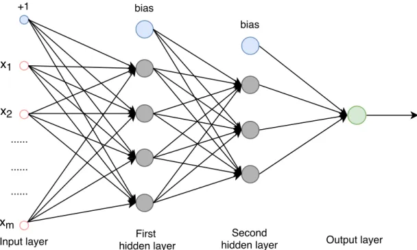
Neural networks are one group of algorithms used for machine learning that model the data using artificial neurons. Neural networks are inspired from biological ner-vous systems. Figure 2.9 illustrates a simple biological neuron network. As can be seen, dendrites bring input signals to neurons, and axons convey the information from the cell body of a neuron to another neuron across synapses. Artificial neural network is one application that applied in computer science based on this biological nervous system, and it is drawn in Figure 2.10. In this figure, there are four layers ℓ: one input layer (in), two hidden layers (hidden) and one output layer (out). The circles that are marked as blue are called bias units. The vectorx= (x1, x2, . . . , xm)

in the leftmost input layer is the input signal that conveyed along the axons. It is moving forward by encoding with the learnable synaptic strengthwℓ

(24)

wℓpq denotes the weights associated with the connection between unit q in current

layerℓ and unitpin previous layer andbℓ represents the bias in current layerℓ. The activation of each unit in the first hidden layer is obtained as below:

ahidden_q =f(∑

p,q

w_pqhiddenxin_p +bin) (2.14)

Thexin

p in Equation 2.14 corresponds to the units in the input layer. The activation

principle of the first hidden layer can be similarly applied into the successive hidden layers. Finally, the dendrites will bring the intermediate operations from the last hidden layer into the output layer where the output will be generated. This neural network defines the hypothesis as below for producing the output:

hw,b =aoutq =f(

∑

p,q

wout_pq ahidden_p +bhidden) (2.15)

Generally, in each unit, the multiplications: w_pqℓ xℓ_p−1 orwℓ_pqaℓ_p−1 are get summed with biasbℓ−1, and followed with an activation functionf. For the activation function, it serves as a decision function which maps the original space into diﬀerent partitions of the output. Various activation functions such as the hyperbolic tangent (TanH) and rectified linear unit (ReLU) activation functions, can be chosen depending on diﬀerent implementation purpose. [33], [34]

(25)

Figure 2.10 A feedforward neural network model.

2.2.2

Back propagation

Backward propagation is a common optimization method of training artificial neural networks. In [35], the good performance of back propagation applications in several neural networks was discussed, and its importance got widely known after that. Back propagation basically has two phases: propagation and weights update.

Propagation: When the neural network is fed with an input, it forward propagates the input through the whole network to output layer where the output is generated. Then the error between desired outputs y_i and predictions yˆ_i of i-th instance is computed from a loss function, which is denoted asL(w, d):

L(w, d) =∑

i

||yˆ_i−y_i||2 (2.16) where the w, d are the weights and biases that we discussed in Subsection 2.2.1. Then the network propagates the error backwards until the weights, connecting all the units between layers, have their corresponding associated error values which represent their contribution to the forward propagation process.

Weights updating: In this phase, based on these error values, backpropagation com-putes the partial derivative ∂wL(w, d) of the loss function L(w, d) with respect to

the weights in the network. The gradient is used to minimize the loss function and get the optimization by updating the weights. This is not merely just a fast learning

(26)

algorithm but also an enlightening process for giving us the insight of how quickly the cost changes and how the weights updating changes the overall behavior of the network.

• Stochastic Gradient Descent

Stochastic Gradient Descent (SGD) is one of the most popular and common algorithms to perform optimization on objective function L(w, d). It updates the weights in the opposite direction of the gradient of objective function L(w, d) which is denoted as:

w =w−η ∂wL(w, d) (2.17)

The learning rate η determines the step size of reaching a valley, and it is typically a small enough number which tends to give good convergence to a local minimum. SGD helps to find a better local optimum by performing frequent updates with a high variance, and to converge to the global minimum ultimately by keeping overshooting. Generally, SGD computes the weights updating using a few training examples or a minibatch from the training set rather than a single example, as this leads to a more stable convergence and eﬃcient matrix operations.

• Adaptive Moment Estimation

In this thesis, we use Adaptive Moment Estimation (ADAM) [36] as the op-timizer of the learning process. It estimates the gradient mean (mt) and

element-wise squared gradient (vt) by employing exponential moving average

while adding bias correction. The biasesβ1, β2 corrected first and second order

moments at time step t are computed as ˆmt and ˆvt:

ˆ mt = mt 1−β1,t , (2.18) ˆ vt = vt 1−β2,t (2.19) The parameters wt+1 at time step t+ 1 are updated by following the ADAM

updating rules as below:

wt+1 =wt− η √ ˆ vt+ϵ ˆ mt (2.20)

whereηrepresents the learning rate, and theϵis a smoothing term that avoids the denominator being zero.

(27)

2.3

Deep learning

Deep learning, also widely known as deep structured learning, is a special branch of machine learning. It is distinguished from the neural networks with single hidden layer by its depth. Technically, the neural networks with more than one hidden layer are considered as deep learning. Each layer of deep learning networks can learn features with diﬀerent abstraction and complexity. The more deeper you go into the deep networks, the more abstract features you can extract from it, this is known as the feature hierarchy.

In this section, the fundamental knowledge of few common remarkable deep neural networks, such as CNNs and RNNs, are presented successively.

2.3.1

Convolutional Neural Networks

Regular neural networks are made up of neurons with learnable weights and biases. The input layer receives a vector input and conveys it across hidden layers which are composed of neurons. The neurons in each layer are fully connected to the neurons in previous layer and next layer, and have no connections with the neurons in the same layer. Such a network structure does not take the spatial structure of the data into account if the input is some spatial one. CNNs perform very well for spatial data, and are able to encode the data properties into architecture.

Figure 2.11 Architecture of Convolutional Neural Network (adapted from [37]).

Generally, the CNN is a sequence of layers, and each layer transforms the volume of activations to the subsequent layer. Basically, the CNN architecture, illustrated in Figure 2.11, has three main layer types which are stacked: convolutional layer, pooling layer and fully-connected layer. CNNs perceive images, assuming the spatial data is image here, as volumes in three dimensions: width, height and depth, which is shown in Figure 2.12. For the input layer, the width and height are measured

(28)

by the number of pixels along x and y coordinates while the depth here is referred as channels, which corresponding to three RGB color space, and illustrated along z coordinate. The input volume is further fed into the network by convolutions. In the convolutional layer, features abstraction is executed with dot product between filter weights and corresponding local input pixels, which is shown in the convolutional layers of Figure 2.11. A two dimensional activation map will be generated by sliding each filter across the width and height of the whole input volume. Usually non-linear activation function, such as ReLU, will be added after each convolutional layer in order to introduce non-linearity into the convolutional network. Depending on the number of filters used in the project, the output of this layer can be created by stacking the activation maps from diﬀerent filters along the dimension: depth. With regard to reducing the workload of the network, the pooling layer, one down sampling operation, usually follows the convolutional layer and decreases the spatial size of its input. After several convolutional and pooling layers, the fully connected layers which fully connect the features with high-abstraction from previous layers come after and finally generate the network output.

Figure 2.12 Three dimensional volume.

CNNs process the spatial and ordered data in an architectural way with three basic concepts: receptive fields, shared weights and pooling technique.

Receptive fields: In CNN, each unit in the hidden layer is only spatially connected to a local region of units in the previous layer, which is called the receptive field for the hidden neuron. Each connection between input pixel within the local receptive field and the hidden neuron learns a weight, and an overall bias is also learned by the hidden neuron. When sliding the local receptive field over the entire input image, there is a specific hidden neuron corresponding to each receptive field in each hidden layer. The size of the local receptive field and the number of hidden layers depends on the kernel size and numbers respectively. To illustrate this concisely in Figure

(29)

2.13, we assume the input is a gray scale image, and the first hidden layer is built up by sliding the local receptive field from the up left corner of the image. Then the local receptive field is slided right or down over the stride length as the model sets.

Figure 2.13 Receptive fields (adapted from [38]).

Shared weights: One principal advantage of CNNs is the shared weights of con-volutional layers, which means that the same weights and biases are used when convolving one filter with diﬀerent local receptive fields. The shared weights and biases achieve better generalization and highly improve the learning eﬃciency by reducing the number of parameters which involved in the convolutional layers. Be-sides, the shared weights also equip the model with the ability of detecting features regardless of their position in the visual field. A feature map is generated after the convolutional operation with this filter. The weights defining the feature maps are called the shared weights, and the biases are called the shared biases. The shared weights and biases define a filter.

Pooling: Pooling layers are typically applied after convolutional layers for down sampling and reducing the spatial size of the output from previous layer. Pooling operation eﬃciently reduces the amount of parameters and computation complexity of network. The most common pooling method is max-pooling. Basically, a pooling window, specifying local pooling areas, is to be set so that you do not need to pool over the entire matrix at one time. For example, the max-pooling of a 2×2 window is a process of traversing over the area within the pooling window and picking up the

(30)

largest element, which is illustrates in Figure 2.14. The output of the max-pooling layer is decreased into a half size matrix with a 2×2 pooling window of stride:2.

Figure 2.14 Maxpooling (adapted from [34]).

2.3.2

Recurrent Neural Networks

RNNs are a type of artificial neural network designed to recognize patterns in se-quences of data, such as sound, written natural language, genomes and stock mar-kets. RNNs were created in 1980’s and started recently gaining popularity in network designs and powerful computation with graphic processing units. One principal dif-ference between RNNs and the traditional neural network is the architecture of how neurons are connected to the others. Each neuron or unit is able to use internal memory to maintain information about the previous input. For example, when you read a message, you understand each word based on your perception of overall context as your memory has persistence.

The reason why RNNs are called recurrentis because RNNs execute the same task on each input element of sequence and produce output based on early computations. A typical recurrent network is shown in Figure 2.15. RNNs allow information to persist by including loops. If unfolding the loops in time, the RNNs can be regard as deep feed forward networks. The chain-like structure is shown in Figure 2.15. xt, st and ot are the input, hidden state and output at time step t, respectively.

U, V are the parameters between input xt and hidden state st, hidden state st and

output ot on current time step t. W is the parameters between successive hidden

states. RNNs share the same parameters across each time step, and this significantly reduces the number of parameters in network. People usually call thestthe memory

(31)

Figure 2.15 A recurrent neural network with unfolding in time (adapted from [39]).

of the network, as it captures the information from the previous time steps. st is

calculated based on the input xt at current time step t and previous hidden state

st−1, which is presented as below:

st=f(U xt+W st−1) (2.21)

The network in Figure 2.15 has outputs at each time step, however, depending on diﬀerent tasks the RNNs can be built diﬀerentiated by operating over sequences. Few examples are illustrated in Figure 2.16. The red circles represent the input vectors, gray ones save the state of RNNs and green stands for output vectors. The arrows indicate the information flowing directions. From 1 to 5, the first ”one to one” is the vanilla model from fixed-sized input to fixed-sized output without RNN. The second ”one to many” model is from fixed-sized input to the sequential output. ”Many to one” models sequential input to the fixed-sized output. Furthermore, the final two ”many to many” models work with the general and synchronized sequence input and sequence output. Compared to the Vanilla Neural Networks which have

(32)

the constraints of fixed-sized input, output and fixed amount of computational steps, the flexibility on operating over sequences of vectors makes RNNs remarkable.

Figure 2.16Examples of Recurrent Neural Network sequential model (adapted from [40]).

The purpose of RNNs is to classify sequential input accurately. It gets the error rate by comparing its predictions with the desired targets from test data. For minimizing this error rate, a gradient based technique called Back Propagation Through Time (BPTT) is applied. BPTT begins by unfolding the RNNs through time as shown in Figure 2.15. BPTT trains and back checks through the network in a sequential order. It significantly faster the process of training RNNs.

RNNs are capable of memorizing the information of arbitrary long sequences in theory, but in practice, st typically cannot capture very long-term dependencies

because of the vanishing gradients problem. Two variants of RNNs: Long Short Term Memory (LSTM) and Gated Recurrent Unit (GRU) are widely used today as the solutions to the vanishing gradients problem. The illustration of LSTM and GRU is shown in Figure 2.17 and discussed as below:

Long Short Term Memory: The LSTM was initially proposed by Hochreiter and Schmidhuber in 1997 [42]. Like all RNNs, a typical LSTM has a chain structure of repeating modules. Each module includes four interactive layers: input gate(it),

(33)

Figure 2.17 Illustration of (a) LSTM and (b) GRU. (adapted from [41])

output gate (ot), forget gate (ft) and cell state gate (ct). The input gate and output

gate regulate the input and output flow of the module. Forget gate layer decides whether to forget or reset the cell state. The cell state gate can be updated optionally by adding or removing information. If feeding sequential data x= (x1, x2, . . . , xn)

to the LSTM network, it will map the input into output by calculating each gate layer equations: ft =σ(Wf ·ht−1+Wf ·xt+bf) (2.22) it=σ(Wi·ht−1+Wi·xt+bi) (2.23) ct=ft⊙ct−1+it⊙tanh(Wc·ht−1+Wc·xt+bc) (2.24) ot =σ(Wo·ht−1+Wo·xt+bo) (2.25) ht=ot⊙tanh(ct) (2.26)

where f, i, o and c are the forget gate, input gate, output gate and cell state gate respectively. t represents the current time step, and ht is the signal that is going

to be output from this module. σ denotes the logistic sigmoid function. All the W

terms are the weights matrices corresponding to each gate of model, and theb terms are biases. ⊙ is an element wise multiplication operation. LSTM unit enables the model to detect and capture the long distance dependencies by deciding whether to save the existing memory through introduced gates or not.

Gated Recurrent Unit: GRU is basically a variant of LSTM having no separate memory cells and output gate. As can be seen from Figure 2.17 (b), r and z represent the reset and update gates whilehand ˜h are the activation and candidate activation operations. Unlike LSTM, the GRU exposes the whole memory state at each time step and balances the previous and new memory states with leaky integration. At time stept, the update gate zt decides how much the previous ht−1

and new memory stateht are to be forgotten or memorized, and is calculated based

(34)

computed by input and the reset gatesrtwith previous memory stateht−1, and this

helps GRU to decide whether the detected features or previous states are necessary or not. [43] The updating and reseting mechanisms are listed as below:

ht= (1−zt)ht−1+ztht (2.27)

zt=σ(Wzit+Uzht−1) (2.28)

˜

ht=tanh(W it+rt⊙U ht−1) (2.29)

rt =σ(Writ+Urht−1) (2.30)

2.4

Existing computational approaches for predicting gene

reg-ulation

Histone modifications are quantizable signals which flank on genes. Multiple re-search and biological technology advancement have capacitated us to profile the quantizable histone modification signals and to quantify the gene regulation more accurately and eﬃciently. Besides, various computational models such as LR, SVM, RF classifier and CNNs have been applied to predict gene expression levels with histone modification signals in last decade.

Research of the correlation between the gene regulation and histone modifications has been done in 2013 by Dong and Weng [3]. LR is a commonly used predictive machine learning model. Its purpose is to furthest minimize the summation of the squared errors of predictions and desired output to fit a straight line into dataset. Article [4] adopted a LR model on data that derived from human T-cell studies [44] to quantify the relation between the histone modifications and gene expression. It showed us that a small number of histone modification signals could make accurate predictions very close to the experiment of using all 38 histone modification marks. It also stressed that the relationship between the histone modification signals and gene regulation is general rather than cell type specific. Furthermore, [45] investigated a hybrid of LR algorithms and applied them to identify the gene regulation patterns by modeling histone modification signals. The authors indicated that the mixture of LR methods have a better performance than using a single LR model.

In 2011, a statistical approach of studying the relationship between gene expression and histone modifications was demonstrated in [5]. Its authors applied SVMs on worm dataset [46] to study the various aspects of gene expression by chromatin features. The regions flanking astride the Transcription Start Site (TSS) and Tran-scription Termination Site (TTS) were divided into bins with 100 basepairs and

(35)

were considered as the features of the SVM models. SVMs are the discriminative classifiers which try to find the hyperplane that gives the maximum margin of the labeled training data (supervised learning). Its results showed the quantitative rela-tionship between the gene regulation and histone modification signals based on the incorporate informations by modeling diﬀerent bins. Besides, it inferred the histone modificaton pairwise interactions with a separate LR model. Bayesian networks were also studied for modeling higher order correlation between the gene expression and histone modification marks.

Dong X built a quantitative model with RF classifiers to predict gene expression levels with histone modification signals in 2012. It performed feature selection by just keeping the bins which correlated with gene expression most, and studied the combinatorial analysis by grouping the 11 histone modifications into 4 functional categories. It proved that the gene expression status can be better predicted by jointing various groups of features. [6]

With the popularity of deep learning recently, deep convolutional networks were pro-posed to predict gene expression levels from histone modifications. In [7], a unified convolutional discriminative framework was developed. This article claimed that the developed DeepChrome model overcame the weaknesses of previous studies such as multiple models, combinatorial analysis and the failure of capturing subtle sequential diﬀerences of histone modification signals. Because the convolutional mechanism in DeepChrome allowed the automatic feature extraction along both the bins direction and histone signals direction. Its result has also shown that the DeepChrome out-performed the discussed early computational methods for predicting gene expression levels with 5 core histone modification signals on 56 cell types.

In conclusion, with the advancement of the biological techniques and development of computational applications of machine learning algorithms, especially the deep learning, the correlation between gene regulation and histone modifications could be modeled more accurately and eﬃciently. This topic is still a rather significative and promising issue as its improvement could support the medicine-health field greatly.

(36)

3.

MATERIALS AND RESEARCH METHOD

3.1

Data Preparation

In this section, the materials and tool that used for generating and processing the data are introduced. Besides, the data extracting and preprocessing process is also discussed.

3.1.1

Materials

Histone modification is a post-translational modification process made on histone proteins which plays a fundamental role in impacting gene regulation [2]. The 5 core histone modification masks: H3K4me3, H3K4me1, H3K36me3, H3K9me3 and H3K27me3 [16], summarized in Table 3.1, and normalized RNA sequence data on 56 cell types are downloaded from Roadmap Epigenomics Mapping Consortium database (REMC) database [16].

Histone Marks Associated with

H3K4me3 Promoter regions

H3K4me1 Enhancer regions

H3K36me3 Transcribed regions H3K9me3 Heterochromatin regions H3K27me3 Polycomb repression regions

Table 3.1 Five core histone modification marks.

GENCODE [47] supports genomics projects by providing updated human gene an-notation. In order to find the gene coordinates in this work, the basic gene annota-tion file is downloaded from the latest version of GENCODE release 25 (mapped to GRCh37).

3.1.2

Bedtools

Bedtools is a powerful and flexible tool that allows various genome arithmetic on diﬀerent genomics analysis tasks [48]. In this work, thebedtools intersect operation

(37)

on the genomic intervals from the 5 core histone modifications and basic gene an-notation file is applied. It provides multiple parameters options for satisfying our diﬀerent needs based on how we expect the intersections operations are reported. This work is done by screening for overlaps between two sets of genomic features usingbedtools intersect.

3.1.3

Data extraction and preprocessing

Based on the gene coordinates that we get from the basic gene annotation file, the ”start location” of the genes with genomic strand ”+” is considered as the TSS, and the ”end location” is considered as TSS with the genes of genomic strand ”-”. For keeping the subtle variations among the eﬀects from histone modification signals on each gene, a 10,000 basepairs DNA region surrounding the TSS is chosen to be mapped into 100 consecutive bins, for which each contains 100 basepairs. [7] The feature window is constructed by intersecting the 5 core histone modification signals with the 100 bins information of each gene from the basic gene annotation file by bedtools intersect operation [48]. Finally, the input of each gene is a 100 × 5 matrix, where the 100 corresponds to the 100 bins and 5 represents the 5 core histone modifications.

3.2

Deep neural network methods

In this decade, deep neural networks have been widely used in many areas be-cause of the remarkable performance. CNNs are powerful in extracting hierarchical features and have made great break through in computer vision domain, such as image classification [8], [9], [49], [50], face recognition [51], [52] and object detec-tion [53], [54], [55]. RNNs are able to learn long term dependencies within data and have shown excellent results [13], [56] in pattern recognition tasks with sequential data.

CNNs are capable of extracting high level features but may fail to learn the long term connectivity about the data while RNNs achieve to model sequential data. [57] In order to preserve the strengths of both the CNNs and RNNs, and to complement their shortcomings, the CNNs and RNNs are combined into a hybrid model which is often referred as the CRNN. The combination of CNNs and RNNs has recently achieved excellent success in many areas such as image representation [58], speech recognition [57], sound event detection [59] and gene expression prediction [17]. In this thesis, we propose a CRNN model and apply it for the gene expression

(38)

Figure 3.1 Architecture of CRNN model(adapted from [17]).

prediction tasks with histone modification signals. Additionally, two simplified ver-sions: CNN and RNN, by removing the recurrent layer and convolutional layers from the CRNN respectively, and the state-of-the-art baseline: DeepChrome [7] are also discussed in this work.

3.2.1

Architecture of CRNN model

In this work, as each gene in our data is a 100×5 matrix, it can be regarded as an image. However, the 100 successive bins probably include dependency information. Thus, we are supposed to design a model that is capable of capturing spatial features while keeping the connectivity information.

We propose a CRNN method which is a hybrid model of CNN and RNN in this thesis. The architecture is presented in Figure 3.1. It consists of seven layers: one input layer, two convolutional layers, one LSTM layer, two fully connected layers and one output layer. After extracting features along both the bin axis and histone axis with the two convolutional layers, the features are mapped into 32 feature maps through ReLU activation function which has been proven to significantly accelerate the convergence of gradient decent [8]. These feature maps are stacked over the

(39)

histone axis before being fed into the LSTM layer. LSTM models long-term depen-dencies of data by using memory cells, and the drop regularization of inputs and recurrent state in the LSTM layer helps to reduce over-fitting. The recurrent layer is followed by two fully connected layers which are connected with ReLU activations. Finally, we get the binary prediction of each gene from the output layer with a sig-moid operator. Gene would be assigned as a high expression level if its prediction belonged to class ”1”, and vice versa. Moreover, in order to alleviate over-fitting, we adopt the dropout operation to each convolutional layer and LSTM layer of our CRNN model.

Figure 3.2 Architecture of CNN model(adapted from [17]).

3.2.2

Baseline models

In this subsection, the architecture of the three comparison models: CNN, RNN and DeepChrome are discussed.

CNN: One simplified variant of CRNN that we will study in this work: CNN, presented in Figure 3.2, is generated by removing the LSTM layer from the ”Region 2” of Figure 3.1. It consists of one input layer, two convolutional layers, two fully connected layers and one output layer.

(40)

Figure 3.3 Architecture of RNN model(adapted from [17]).

(41)

RNN: RNN is another simplified version of CRNN by removing the convolutional layers, denoted in ”Region 1” of Figure 3.1. It is a model of one input layer followed with a LSTM layer, two dense layers and one output layer successively, which is illustrated in Figure 3.3.

DeepChrome: Singh introduced a convolutional network model named DeepChrome in [7], which is a model of one convolutional layer followed with a maxpooling op-erator, one dropout layer, two dense layers and one output layer. Additionally, the ReLU activation function is applied on the convolutional layer and dense layers for sparsity and reducing the likelihood of the gradient to vanish, and the sigmoid ac-tivation function is adopted in output layer for the final binary prediction in this work. Its architecture is shown in Figure 3.4.

(42)

4.

RESULTS AND DISCUSSION

In this chapter, the diﬀerent evaluation methods are introduced firstly. Then the experiments and their corresponding evaluation results are discussed. The analyses of theGene Expression Prediction competition, which follows, are discussed in the end of this chapter.

4.1

Evaluation methods

4.1.1

Receiver Operating Characteristic

Receiver Operating Characteristic (ROC) curve is a fundamental and statistical tool for the evaluation of model performance. [60], [61] It is a commonly used way to quantify and visualize the performance of a binary classifier. There are four important concepts from a binary classifier when the two classes are labeled as positive ”+1” and negative ”-1”:

• True Positive (TP): positive value is predicted to be positive.

• False Positive (FP): negative value is predicted to be positive.

• True Negative (TN): negative value is predicted to be negative.

• False Negative (FN): positive value is predicted to be negative.

A confusion matrix of binary classifier can be made in Figure 4.1 based on the above four terms, and several error matrices such as True Positive Rate (TPR) and False Positive Rate (FPR) are derived from the confusion matrix,

T rueP ositiveRate(T P R) = T P T P +F N = T P P (4.1) F alseP ositiveRate(F P R) = F P F P +T N = F P N (4.2)

(43)

Figure 4.1 Confusion matrix.

TPR tells us how often does it predict ”positive” when it is actually ”positive”, and also known as ”sensitivity” or ”recall”. The FPR shows how often does it predict ”positive” when it is actually ”negative”, and it can be calculated as 1 -”specificity”, where the ”specificity” indicates how often does it predict ”negative” when it is actually ”negative”. [62]

ROC curve is generated by graphically plotting the TPR against the FPR while varying possible thresholds for assigning observations to the given classes. Figure 4.2 shows an example distribution of predicted probabilities of each class. The green and blue curves visualize the diﬀerence between the predicted probabilities and true statues. If we assume the height at probability: 0.3 is 40, at 0.5 is 10, it means that the probability of predicting the 40 samples to be positive are 0.3, and the true status for all the 40 items is negative. There are about 10 samples for which we predict a probability of 0.5, and half of them are positive and the other half are negative. Based on this example, we think that this classifier works good as it separates the classes well. Its ROC curve over all possible thresholds is drawn in Figure 4.3. In a ROC, the TPR is graphically plotted in function of the FPR for various decision thresholds. For example, if we set the threshold at 0.0 where is the black bar located in the distribution of predicted probabilities, the classifier classifies all items as positive (TPR = 1.0, FPR = 1.0) which corresponds to the red point at the top-right corner of the ROC curve in Figure 4.3. If dragging the threshold right, the corresponding TPR-FPR point will move to the left and down side. When

(44)

the threshold moves to 0.5 which is the default setting of most classifiers, all of the items above 0.5 are predicted as positive and the ones below 0.5 are negative. Its TPR-FPR point moves to the top-left corner (green point) of the ROC curve.

Figure 4.2 Distribution of predicted probabilities.

Figure 4.3 ROC curve for the first distribution example.

The given example in Figure 4.2 is a classifier that works good for classifying the two classes well. However, finding an optimal classifier usually takes time in reality.

(45)

The classification accuracy will become lower when the overlap between the two distributions becomes larger by moving the green distribution right, which is shown in Figure 4.4. This happens regardless of where we set the threshold. Its ROC curve can be generated by plotting the TPR versus FPR by varying all possible thresholds which range from 0 to 1.0. We can get even worse performance by moving the green distribution righter which is presented in Figure 4.5. This classifier does a pretty poor classification with a ROC curve that is close to the diagonal line which denotes random guessing. It infers that the performance of this classifier is no better than the random case.

Figure 4.4 ROC curve for the second distribution example.

Figure 4.5 ROC curve for the third distribution example.

In Figure 4.6, the red ROC curve that hug the up left corner of the plot is the optimal one. The classifiers perform worse if their ROC curves are more closer to the black diagonal dashed line which represents the random guessing. The ROC curves are commonly used for visualizing and comparing the performance of classifier

(46)

methods. Moreover, Area Under the Curve (AUC) is a good way of quantifying the performance of a classifier from ROC. AUC is literally the percentage of the area under the curve. Its value ranges from 0 to 1.0. The larger the AUC scores are, the better the classifiers perform. Furthermore, the AUC is a very useful method when the dataset is highly unbalanced and when the predicted probabilities have a large variance or a ”smooth” distribution. [61], [63]

Figure 4.6 Comparison of ROC curves.

4.1.2

P-value

P-value is used to determine statistical significance in a hypothesis test. Null hypoth-esis is an essential concept for the interpretation of p-values. For each experiment, there is the difference between groups that the researchers are testing. In this work, the groups could be the effectiveness of the different studied models. It is always possible that the lack of difference happens between the groups, which is called the null hypothesis. A p-value is the probability of occurrence of an observed result when we assume the null hypothesis is true. Graphically, the p-value is the shaded magenta area in the tail of probability distribution, where the portion under the curve that past the observed point. It is illustrated in Figure 4.7.

(47)

Figure 4.7 P-value.

P-value manages how compatible our data is with the null hypothesis. The alter-native hypothesis is the opposite of the null hypothesis. In other words, alteralter-native hypothesis is the one we believe when the null hypothesis is predicted to be untrue. A low p-value indicates that our data instances provide enough evidence that there is a significant diﬀerence between the compared groups. Hypothesis tests adopt a p-value to weigh the strength of the evidence, and are expressed as decimals to demonstrate the probabilities that the results could be random. There is a term named significance level (α) which is used to refer to a predefined probability while the term p-value is used to indicate a probability that we calculate from the experi-ment work. Conventionally, the significance levels of 5%, 1% and 0.1% are commonly set by researchers before examining the data instead of deriving from observational data or underlying hypothesis. A value of 5% is chosen forαin our work empirically. The p-value is range from 0 to 1.0 and interpreted as follows:

A low p-value (≤ α) manifests strong evidence against the null hypothesis so that we could reject the null hypothesis.

A high p-value (≥ α) manifests no significant result against the null hypothesis so that we fail to reject the null hypothesis.

(48)

A p-value close to significance level (α) is considered to be marginal.

Therefore, the smaller the p-value is, the more important our result is. Because it indicates that the null hypothesis under consideration probably fails to explain the observation adequately.

4.2

Experiments

The data that derived in Section 3.1 includes 19356 genes of 56 cell types. Thus, our task in this work is to develop a general model that can accurately predict gene expression levels from histone modification signals over 56 cell types. For each cell type, there are 19356 genes, and we use this data for training, validation and testing. Specifically, we partition 60% of all genes of each cell type from the dataset into training set, 20% of all genes into validation set and 20% into test set. Furthermore, we implement the studied models by Keras1 with Theano2.

We evaluate the proposed CRNN model with the histone modification signals and gene expression data from 56 cell types. Its performance is compared to two sim-plified variants: CNN and RNN, and baseline: DeepChrome which are discussed in Subsection 3.2.2. In the CRNN model, each convolutional layer uses 3×3 filter kernels and a stride of 3. The number of filters we choose for each convolutional layer is 32. Two fully connected layers with 100 and 20 nodes follow a LSTM layer which includes 32 units. The dropout strategy with 50% probability is applied to avoid network over-fitt