AnD: A Many-Objective Evolutionary Algorithm with Angle-based Selection and Shift-based Density Estimation
Zhi-Zhong Liu, Yong Wang, Pei-Qiu Huang
PII: S0020-0255(18)30512-7
DOI: 10.1016/j.ins.2018.06.063
Reference: INS 13756
To appear in: Information Sciences
Received date: 17 April 2018
Revised date: 21 June 2018
Accepted date: 29 June 2018
Please cite this article as: Zhi-Zhong Liu, Yong Wang, Pei-Qiu Huang, AnD: A Many-Objective Evolu-tionary Algorithm with Angle-based Selection and Shift-based Density Estimation,Information Sciences
(2018), doi:10.1016/j.ins.2018.06.063
This is a PDF file of an unedited manuscript that has been accepted for publication. As a service to our customers we are providing this early version of the manuscript. The manuscript will undergo copyediting, typesetting, and review of the resulting proof before it is published in its final form. Please note that during the production process errors may be discovered which could affect the content, and all legal disclaimers that apply to the journal pertain.
ACCEPTED MANUSCRIPT
Highlights
• We design AnD as an alternative MaOEA, which has a simple structure, few parameters, and no complicated operators. More importantly, AnD is different from existing methodsit does not use dominance rules, weight vec-tors/reference points, and indicators.
• To the best of our knowledge, it is the first attempt to effectively com-bine vector angle with shift-based density estimation for solving MaOPs, by making use of their complementary properties.
• We compared AnD with other seven state-of-the-art MaOEAs on a variety of benchmark test problems with up to 15 objectives. The results provide evidence that AnD can achieve highly competitive performance.
• AnD has been further extended to solve constrained MaOPs with promising performance
ACCEPTED MANUSCRIPT
AnD: A Many-Objective Evolutionary Algorithm
with Angle-based Selection and Shift-based
Density Estimation
Zhi-Zhong Liua, Yong Wanga,b,∗, Pei-Qiu Huanga
aSchool of Information Science and Engineering, Central South University, Changsha 410083,
China.
bSchool of Computer Science and Electronic Engineering, University of Essex, Colchester CO4
3SQ, UK.
Abstract
Evolutionary many-objective optimization has been gaining increasing attention from the evolutionary computation research community. Much effort has been de-voted to addressing this issue by improving the scalability of multiobjective evo-lutionary algorithms, such as Pareto-based, decomposition-based, and indicator-based approaches. Different from current work, we propose an alternative algo-rithm in this paper called AnD, which consists of anangle-based selection strategy and a shift-baseddensity estimation strategy. These two strategies are employed in the environmental selection to delete poor individuals one by one. Specifically, the former is devised to find a pair of individuals with the minimum vector angle, which means that these two individuals have the most similar search directions. The latter, which takes both diversity and convergence into account, is adopted to compare these two individuals and to delete the worse one. AnD has a sim-ple structure, few parameters, and no complicated operators. The performance of AnD is compared with that of seven state-of-the-art many-objective evolution-ary algorithms on a variety of benchmark test problems with up to15objectives.
The results suggest that AnD can achieve highly competitive performance. In addition, we also verify that AnD can be readily extended to solve constrained many-objective optimization problems.
Keywords: Evolutionary algorithms, many-objective optimization, angle-based ∗Corresponding author.
ACCEPTED MANUSCRIPT
selection, shift-based density estimation 1. Introduction
Multiobjective optimization problems (MOPs) refer to optimization problems with more than one conflicting objective. Usually, a MOP can be expressed as:
minimizeF(x) = (f1(x), f2(x), ..., fm(x))
subject tox ∈ Ω (1)
wherex= (x1, x2, ..., xn)is the decision vector,nis the number of decision
vari-ables, F(x) is the objective vector, m is the number of objectives, and Ω is the
decision space. The ultimate goal of multiobjective optimization is to obtain a set of well-distributed and well-converged nondominated solutions to approximate the Pareto front (PF). To achieve this goal, numerous multiobjective evolutionary algorithms (MOEAs) have been proposed over the last few decades. Accord-ing to their selection mechanisms, MOEAs can be roughly classified into three categories: Pareto-based methods, decomposition-based methods, and indicator-based methods [44]. MOEAs have shown great potential to solve MOPs with two or three objectives. However, for MOPs with more than three objectives, often known as many-objective optimization problems (MaOPs), they encounter sub-stantial difficulties [19].
For Pareto-based methods, such as NSGA-II [9] and SPEA2 [46], the sele-ction criteria (i.e., the Pareto-based selesele-ction and the diversity-based selesele-ction) may lose their effectiveness to push the population toward the PF. This is because with an increase in the number of objectives, the proportion of nondominated solutions increases drastically. As a result, the Pareto-based (primary) selection fails to distinguish the individuals in the population. Under this condition, the diversity-based (secondary) selection will play a major role in the selection pro-cess. The secondary selection may distribute the population well over the ob-jective space; however, the population tends to be far away from the desired PF due to the neglect of convergence performance. Decomposition-based [42] and indicator-based [2] methods do not suffer from selection pressure issues since they do not rely on Pareto dominance to evolve the population. However, they face their own challenges. Regarding decomposition-based methods, it is not a trivial task to assign the weight vectors or reference points in the high-dimensional objective space [22]. In addition, indicator-based methods always result in high computational time complexity [33].
ACCEPTED MANUSCRIPT
To enhance the scalability of MOEAs for MaOPs, a considerable number of at-tempts have been made to improve the performance of Pareto-based, decomposition-based, and indicator-based methods. These are briefly introduced next.
• Pareto-based Methods: Recognizing the drawback of the Pareto-dominance relation for MaOPs, this kind of method intends to modify/relax the defi-nition of Pareto dominance. Along this line, several rules have been pro-posed such as-dominance [23], L-dominance [48], and fuzzy dominance [34].
Additionally, another avenue is to develop customized diversity mecha-nisms, with the purpose of alleviating the loss of selection pressure. In [1], a diversity management mechanism is introduced, which can determine whether or not to activate diversity promotion based on the distribution of population. In [27], a shift-based density estimation strategy is proposed, which shifts the poorly converged individuals into crowded regions and as-signs them high density values. As a result, these individuals are very likely to be removed from the population. Inspired by the idea that the knee points are naturally most preferred among nondominated solutions, a knee point-driven EA is proposed in [43], in which diversity is embedded in the knee point identification process.
• Decomposition-based Methods: This kind of method contains two different types. The first type decomposes a MaOP into a series of single-objective optimization problems. MOEA/D [42] is the most famous one. In MOEA/D, a set of weight vectors are predefined to specify multiple search directions toward the PF. Since the search directions spread out widely, it is expected that the obtained solutions cover the PF well. MOEA/D was originally designed for solving MOPs. Recent advances have successfully adapted MOEA/D to solve MaOPs. Examples include adaptively allocating search effort in MOEA/D-AM2M [28], exploiting the perpendicular distance from the solution to the weight vector in MOEA/D-DU [41], and using Pareto adaptive scalarizing methods in MOEA/D-PaS [38]. The second type di-vides a MaOP into a group of sub-MaOPs. One representative is NSGA-III [8], which makes use of a set of predefined well-distributed reference points to manage nondominated solutions. That is, the nondominated solu-tions close to the reference points are prioritized. For these two types, to achieve good performance, a crucial issue is how to assign the appropriate weight vectors or reference points. To this end, an automatic weight vector generation system is devised in [18], and a two-layered generation strategy for reference points is proposed in [8].
ACCEPTED MANUSCRIPT
• Indicator-based Methods: In this kind of method, the indicator values are used to guide the search process. Among all the indicators, the hypervol-ume indicator [47] is the most commonly used, which is originally a quality indicator to compare different MOEAs. The hypervolume indicator has an attractive property, that is, it is strictly monotonic with regard to Pareto dom-inance [2]. Note, however, that the burden for calculating hypervolume is very high, and increases exponentially as the number of objectives increa-ses. To overcome this shortcoming, the Monte Carlo simulation is employed in [2] to approximate the exact hypervolume values, with the aim of striking a tradeoff between accuracy and computational time. Additionally, there are some cheap indicators, such as theI()+ indicator in IBEA [45] and theR2
indicator inR2-EMOA [32]. The collaboration of different cheap indicators
seems to be a promising direction for solving MaOPs [25].
Apart from these three categories, several preference-based many-objective EAs (MaOEAs) have been proposed recently [37, 13] which focus on a subset of the PF based on the user’s preference. There are also some dimensionality reduc-tion approaches [30, 29, 14], aiming to deal with MaOPs with redundant objec-tives. Additionally, researchers have tried to take advantage of the merits of-fered by different categories. Two representatives are MOEA/DD and Two Arch2. MOEA/DD [26] is based on Pareto dominance and decomposition, and Two Arch2 [35] is based on Pareto dominance and an indicator. For more information about MaOEAs, interested readers are referred to a survey paper [24].
Unlike recent work, we propose an alternative MaOEA, called AnD. In evo-lutionary many-objective optimization, the task of environmental selection is to choose some promising individuals from the union population, which is composed of the parent and offspring populations, for the next generation. AnD tackles this task by two strategies: angle-based selection and shift-baseddensity estimation. First, angle-based selection finds a pair of individuals with the minimum vector angle. Intuitively, it is necessary to delete one of these two individuals since they search in the most similar directions and it will waste significant computational resources if they coexist. In order to make the deletion wiser, we need to take both convergence and diversity into account since achieving balance between conver-gence and diversity is the most important concern in many-objective optimization. Fortunately, shift-based density estimation has the capability to cover both the dis-tribution and convergence information of individuals [27]. Therefore, it is utilized to compare these two individuals and to delete the worse one. By repeating this process, AnD provides a quite natural way for solving MaOPs—the individuals
ACCEPTED MANUSCRIPT
with poor diversity and convergence are eliminated from the union population one by one.
The main contributions of this paper are summarized as follows:
• We design AnD as an alternative MaOEA that has a simple structure, few parameters, and no complicated operators. More importantly, AnD is differ-ent from existing methods because it does not use dominance rules, weight vectors/reference points, and indicators. As a consequence, it has the fol-lowing advantages for solving MaOPs: no disadvantages incurred from in-sufficient selection pressure as in Pareto-based methods, no need to assign weight vectors/reference points as in decomposition-based methods, and no need to consume a high computational cost as in indicator-based methods. • The vector angle [4, 40] and shift-based density estimation [27, 36] have
been extensively investigated in the design of MaOEAs, respectively. How-ever, to the best of our knowledge, ours is the first attempt to effectively combine them together for solving MaOPs, by making use of their com-plementary properties. Moreover, AnD provides a straightforward way to achieve both diversity and convergence—by identifying the two individuals with the minimum vector angle via angle-based selection and removing the one with worse diversity and convergence via shift-based density estimation in an iterative way.
• Systematic experiments have been conducted on both the DTLZ and WFG test suites to demonstrate the effectiveness of AnD. The performance of AnD is compared with that of seven state-of-the-art MaOEAs. The experi-mental results suggest that, overall, AnD can achieve better performance in terms of two widely used performance metrics: IGD [5] and HV [47]. • AnD has been further extended to solve constrained MaOPs with promising
performance.
The rest of this paper is organized as follows. Section 2 introduces prelimi-nary knowledge. The details of AnD are presented in Section 3. Subsequently, the experimental setup is described in Section 4. The empirical results on both unconstrained and constrained MaOPs are given in Section 5. Finally, Section 6 concludes this paper.
ACCEPTED MANUSCRIPT
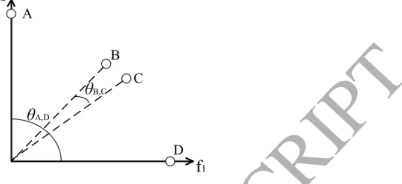
A B C D f2 f1 θA,D θB,CFigure 1: Illustration of the vector angle in a bi-objective minimization scenario
2. Preliminary Knowledge 2.1. Vector Angle
In this paper, the vector angle denotes the included angle between two in-dividuals in the normalized objective space. The normalized objective vector of an individual is computed as follows. First, we find the ideal pointZmin =
(zmin
1 , z2min, ..., zmmin)and estimate the nadir point asZmax = (z1max, zmax2 , ..., zmmax),
wherezmin
i andzimax are the minimum and maximum values of theith objective
of all individuals, respectively. Afterward, for thejth individualxj, its objective
vectorF(xj)is normalized asF 0 (xj) = (f 0 1(xj), f 0 2(xj), ..., f 0 m(xj))according to fi0(xj) = fi(xj)−zimin zmax i −zimin , i = 1,2, ..., m. (2)
After the normalization, the vector angle between two individualsxj and xl,
re-ferred to asθxj,xl, is computed as θxj,xl =arccos F0 (xj)•F 0 (xl) kF0(xj)k × kF 0 (xl)k . (3) whereF0 (xj)•F 0
(xl) denotes the inner product of F 0
(xj) and F 0
(xl), and k · k
calculates the norm of a vector. It is clear thatθxj,xl ∈
0,π
2
.
In principle, the vector angle reflects the similarity of search directions be-tween two individuals. To be specific, if two individuals search in quite different directions, the vector angle between them is large; otherwise, the vector angle is
ACCEPTED MANUSCRIPT
small. Fig. 1 gives an example. From Fig. 1, we can observe that: 1) individuals Aand Dsearch in quite different directions, andθA,D is relatively larger; and 2)
individualsBandCshare similar search directions, andθB,Cis relatively smaller.
During the past two years, the vector angle has attracted a high level of inter-est for evolutionary many-objective optimization. For instance, it has been incor-porated into decomposition-based approaches. In [4], a reference-vector-guided EA (RVEA) for many-objective optimization is proposed. In RVEA, the angle-penalized distance is used to balance the convergence and diversity of individuals in the high-dimensional objective space. In [39], a novel decomposition-based MaOEA called MOEA/D-LWS is proposed. In MOEA/D-LWS, for each search direction, the optimal solution is selected only among its neighboring solutions. Note that the neighborhood is defined by a hypercone, whose apex angle is de-termined automaticallya priori. Very recently, a new variant of MOEA/D with
sorting-and-selection (MOEA/D-SAS) has been presented [3]. In MOEA/D-SAS, the balance between convergence and diversity is achieved by two distinctive com-ponents: decomposition-based sorting and angle-based selection. In the latter, the angle information between two individuals in the objective space is used to maintain diversity. In addition, the vector angle also has the potential to improve the performance of Pareto-based approaches. In [40], a vector-angle-based EA (VaEA) for unconstrained many-objective optimization is developed. VaEA im-plements the nondominated sorting procedure to obtain different layers, and deals with the last layer through the vector angle.
Other kinds of attempts have also been made to solve MaOPs with the use of the vector angle. For example, He and Yen [15] suggested a MaOEA based on a coordinate selection strategy (MaOEA-CSS), in which a new diversity measure based on the vector angle is designed in the mating and environmental selection.
2.2. Shift-based Density Estimation
Shift-based density estimation is an advanced density estimation strategy pro-posed by Liet al.[27]. Compared with traditional density estimation, it shifts the positions of other individuals when estimating the density of an individual (e.g., xj) in the population P. This shift process is simple and is based on the
con-vergence comparison between other individuals andxj on each objective. To be
specific, ifxl (suppose that xlis another individual inP) outperformsxj on one
objective, its objective value on this objective will be shifted to the same position ofxj on this objective; otherwise, its objective value remains unchanged. This
ACCEPTED MANUSCRIPT
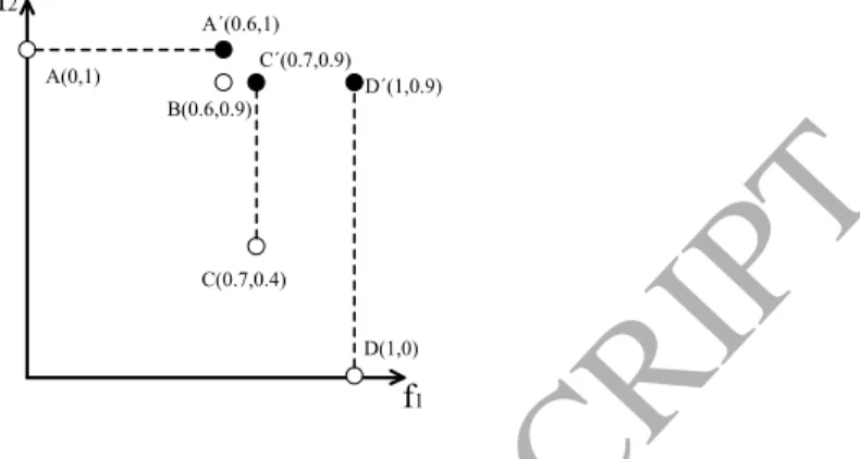
A(0,1) B(0.6,0.9) C(0.7,0.4) D(1,0) f1 f2 A´(0.6,1) C´(0.7,0.9) D´(1,0.9)Figure 2: Illustration of shift-based density estimation in a two-dimensional normalized objective space. To estimate the density of individualB, the other individualsA,C, andDare shifted toA0,
C0, andD0, respectively.
shift process can be described as
fis(xl) = ( fi0(xj), iff 0 i(xl)< f 0 i(xj) fi0(xl), otherwise . (4) wherefs
i(xl)is the shifted objective value off 0
i(xl), andFs(xl) = (f1s(xl), f2s(xl), ..., fs
m(xl)) is the shifted objective vector ofF 0
(xl). Note that before shifting, the
objective vector of each individual is normalized via Eq. (2).
To understand the shift process more clearly, we take shift-based density es-timation of individual B(0.6,0.9) in Fig. 2 as an example. First, individuals
A(0,1), C(0.7,0.4), and D(1,0) in Fig. 2 are shifted to individuals A0(0.6,1),
C0(0.7,0.9), andD0(1,0.9), respectively, due to the fact thatA
1 = 0 <B1 = 0.6, C2 = 0.4< B2 = 0.9, andD2 = 0< B2 = 0.9. Subsequently, it can be observed that the poorly converged individual Bis located in a crowded region. Thus, B will be assigned a high density value and is very likely to be removed from the population. It is noteworthy that in order to obtain the density of an individual, the shift process should be combined with a density estimator, such as the crowd-ing distance in NSGA-II [9], thekth nearest neighbor in SPEA2 [46], or the grid crowding degree in PESA-II [6]. Actually, as pointed out in [27], only the individ-ual with both good diversity and good convergence will have a low density value, which means that both diversity and convergence are elaborately considered in the shift-based density estimation strategy.
ACCEPTED MANUSCRIPT
In this paper, we integrate shift-based density estimation with thekth nearest
neighbor to estimate the density of individualxj inP, denoted as SD(xj). The
implementation is the following:
1. Shift the normalized objective vectors of the other individuals in P via Eq. (4);
2. Calculate the Euclidian distances between the other shifted normalized ob-jective vectors andF0
(xj)according to: d(xj,xl) =kFs(xl)−F
0
(xj)k,xl∈ P ∩xl 6=xj. (5)
3. Find thekth minimum value`(xk)in the set of{d(xj,xl),xl∈ P ∩xl 6=xj},
wherekis set to√N andN is the size ofP; 4. ComputeSD(xj)according to Eq. (6):
SD(xj) =
1 `(xk) + 2
. (6)
Note that the higher the density value, the worse the performance of an individual. The shift-based density estimation strategy has become an important tech-nique in evolutionary many-objective optimization. From [27], it can significantly enhance the scalability of NSGA-II [9], SPEA2 [46], and PESA2 [6] for solv-ing MaOPs. Moreover, SPEA2 achieves better performance than NSGA-II and PESA2 after these three algorithms are integrated with shift-based density esti-mation. Recently, Wanget al.[36] presented a cooperative differential evolution with multiple populations (CMODE) for multi- and many-objective optimization. From the results, the combination of CMODE and shift-based density estima-tion reaches outstanding performance when solving MaOPs. Very recently, Li
et al.[25] presented a stochastic ranking-based multi-indicator algorithm (SRA). SRA adopts the stochastic ranking technique to balance the search biases of dif-ferent indicators. Among these indicators, one is designed based on shift-based density estimation.
3. Proposed Approach 3.1. AnD
The framework of AnD is given inAlgorithm 1. First, a populationP0with
N individuals is randomly initialized in the decision spaceΩ. During the
ACCEPTED MANUSCRIPT
Algorithm 1The framework of AnD
Input: a MaOP and the population sizeN
Output: the populationP 1: Initialization(P0);
2: t←0
3: whilethe stopping criterion is not metdo
4: Qt←Mating(Pt);
5: Ut← PtSQt;
6: Pt+1←Enviromental-Selection(Ut)
7: t←t+ 1; 8: end while
a union population Ut is obtained by combining Qt with Pt. Finally, the
envi-ronmental selection is performed onUt to produce the next populationPt+1. The above procedure repeats until the stopping criterion is met.
It can be seen that similar to most MaOEAs, AnD involves two main compo-nents: mating and environmental selection. The aim of mating is to generate a number of offspring (i.e.,Qt) from the parents (i.e.,Pt) by making use of evolu-tionary operators, such as selection, crossover, and mutation. AnD does not apply any explicit selection to choose parents fromPt or employ any special crossover and mutation to generate offspring. Instead, the parents are randomly chosen from
Pt, and the simulated binary crossover (SBX) and the polynomial mutation are
uti-lized to generateQt. The reasons are twofold: 1) the random selection, SBX, and
the polynomial mutation have been widely used in the community of evolutionary many-objective optimization; and 2) we would like to ensure a fair comparison with other algorithms. The unique characteristic of AnD lies in its environmental selection, which is described in the sequel.
3.2. Environmental Selection
The environmental selection aims at choosing N individuals with the most potential from the union populationUtfor the next generation. AnD accomplishes this by two strategies: angle-based selection and shift-based density estimation.
Algorithm 2 describes the environmental selection of AnD. Firstly, the vector
angles between any two individuals inUt are calculated. Thereafter, angle-based selection is conducted to identify two individuals (denoted as uj and ul) with
the minimum vector angle in Ut. Subsequently, shift-based density estimation is employed to compare uj and ul, and the one with a higher density value is
ACCEPTED MANUSCRIPT
Algorithm 2Environmental-Selection(Ut)
Input: Utwhich is the union ofPt andQt Output: Pt+1
1: Calculate the vector angles between any two individuals inUt based on Section 2.1; 2: while|Ut|> N do
3: Find two individuals (denoted asujandul) with the smallest vector angle inUt; 4: CalculateSD(uj)andSD(ul)according to Section 2.2;
5: ifSD(uj)< SD(ul)then
6: Ut← Ut\ul; // deleteulfromUt
7: else
8: Ut← Ut\uj; // deleteujfromUt 9: end if
10: end while
11: Pt+1← Ut;
removed fromUt. This process proceeds until the size ofUt is equal toN. Next,
we explain the importance of the combination of these two strategies in AnD. As mentioned in Section 2.1, the vector angle reflects the similarity between two individuals in their search directions. If two individuals share the minimum vector angle, they absolutely have the most similar search directions. To improve the diversity of search directions, one of them should be discarded. If we re-peatedly delete one of two individuals with the most similar search directions in the remaining population, the diversity of search directions will be well main-tained in the final population. Indeed, the main idea behind angle-based selection is to approximate the PF from diverse search directions. Decomposition-based approaches, which have shown great success in solving MaOPs, also use a simi-lar idea. However, compared with decomposition-based approaches, angle-based selection only exploits the information provided by the vector angle.
Although angle-based selection is able to find a pair of individuals with the most similar search directions, it cannot distinguish them. In many-objective op-timization, when comparing two individuals, it has been widely accepted that both diversity and convergence should be considered. Fortunately, shift-based density estimation provides an effective way to measure the quality of two individuals because it focuses on both the diversity and convergence of individuals as intro-duced in Section 2.2. As a result, shift-based density estimation has the capability to judge which individual is worse and should be deleted under this condition.
Overall, the environmental selection of AnD combines angle-based selection and shift-based density estimation in a quite natural way: the former identifies the
ACCEPTED MANUSCRIPT
A(0,0.9) B(0.7,1) C(1,0.3) D(0.7,0.15) E(0.9,0.05) F(1,0) f1 f2(a) NSGA-III and SPEA2+SDE
A(0,0.9) B(0.7,1) C(1,0.3) D(0.7,0.15) E(0.9,0.05) F(1,0) f1 f2 w1 w2 w3 w4 (b) MOEA/D A(0,0.9) B(0.7,1) C(1,0.3) D(0.7,0.15) E(0.9,0.05) F(1,0) f1 f2 w1 w2 w3 w4 (c) MOEA/DD A(0,0.9) B(0.7,1) C(1,0.3) D(0.7,0.15) E(0.9,0.05) F(1,0) f1 f2 R(1.1,1.1) Reference point (d) HypE A(0,0.9) B(0.7,1) C(1,0.3) D(0.7,0.15) E(0.9,0.05) F(1,0) f1 f2 (e) AnD
Figure 3: Illustration of the working principles of six MaOEAs. There are six individuals in the population, i.e.,A,B,C,D,E, andFand the task is to select four promising individuals for the next generation.
ACCEPTED MANUSCRIPT
two most similar individuals in terms of search direction, and the latter eliminates the worse one in terms of both diversity and convergence. Therefore, by iteratively implementing both of them, the individuals with poor diversity and convergence are deleted one by one fromUt; thus, the population continuously approaches the PF with good diversity.
3.3. Analysis of the Principle
An example in a two-dimensional objective space is used to illustrate the working principles of six MaOEAs: NSGA-III [8], SPEA2+SDE (a combination of SPEA2 and shift-based density estimation) [27], MOEA/D [42], MOEA/DD [26], HypE [2], and AnD. Suppose that there are six individuals (i.e.,A(0,0.9),B(0.7,1), C(1,0.3),D(0.7,0.15),E(0.9,0.05), andF(0,1)) in the population, and our task is to select four promising individuals for the next generation. Fig. 3 depicts what happens to the six compared methods.
From Fig. 3, we can give the following comments:
• In both NSGA-III and SPEA2+SDE,A,D,E, andFare selected for the next generation. The reason is that these two algorithms prefer nondominated individuals. From Fig. 3(a), it can be observed that Bis Pareto dominated by Aand D, andCis Pareto dominated by D, E, andF. Thus, A, D, E, andFare the nondominated individuals, whileBand Care the dominated individuals.
• With respect to MOEA/D, suppose that there are four weight vectors (i.e., w1,w2,w3, andw4) as shown in Fig. 3(b), and that the Tchebycheff approach is used. According to the principle of MOEA/D with the Tchebycheff approach, each weight vector is associated with an individual. From Fig. 3(b), it is clear thatw1andw2are associated withA;w3is associated withD; and w4 is associated with F. Therefore, A, DandFwill survive into the next generation. In particular,Awill be duplicated. The other individuals (i.e., B,C, andE) will be eliminated.
• For MOEA/DD,A,B,C, andFwill survive into the next generation. This is because the weight vectors in MOEA/DD are used to divide the objective space into a series of subregions. From Fig. 3(c), we can see thatA,B, and Care in their own isolated subregions, and all of them will be selected into the next generation. D, E, andFare in the same subregion, and only the boundary individualFwill be chosen for the next generation.
ACCEPTED MANUSCRIPT
• In terms of HypE, like NSGA-III and SPEA2+SDE,A,D,E, andFremain, and the others are deleted. The reason is becauseBandCdo not contribute to the whole population’s hypervolume value, while the other individuals (i.e., A, D, E, and F) do contribute. As a result, Band C are eliminated from the population.
• To implement AnD, firstly, it is necessary to calculate the vector angles be-tween any two individuals in the population. Subsequently, we need to iden-tify two individuals with the minimum vector angle and employ the shift-based density estimation strategy to differentiate them. It is easy to find that
θE,Fis the minimum vector angle in the population. Then, according to
Sec-tion 2, we can obtain the density values ofEandFasSD(E)≈0.4762and SD(F)≈ 0.4651, respectively. Thus,Ewill be removed from the
popula-tion since it has the higher density value. AfterEhas been eliminated,θC,D
becomes the minimum vector angle and the density values of Cand Dare computed asSD(C) = 0.5andSD(D)≈0.4348, respectively. Thereafter, Cwill be removed from the population due to its higher density value. In summary, Cand Ewill be eliminated from the population, whileA,B, D, andFwill be chosen for the next generation.
From the above discussions, we can observe that:
• The principle of AnD is different from that of the other five state-of-the-art MaOEAs. AnD employs two simple strategies, namely angle-based sele-ction and shift-based density estimation, to delete the inferior individuals one by one from the population.
• AnD can obtain more suitable results compared with the five competitors. In NSGA-III, SPEA2+SDE, and HypE,A,D,E, andFsurvive into the next generation. In terms of MOEA/D,A,D, andFremain. In particular,Ais copied. With respect to MOEA/DD,A,B,C, andFare chosen for survival. However, only in AnD, A, B, D, and F are selected for the next genera-tion simultaneously. Note thatBplays an important role in maintaining the diversity of search directions since it is in a sparse region. Nevertheless, only in AnD and MOEA/DD, it survives. In contrast to MOEA/DD, AnD keeps Dand deletes C. This seems more reasonable sinceCand D share similar search directions butDhas better convergence performance. Conse-quently, we demonstrate how AnD is able to strike a better balance between convergence and diversity than the five competitors.
ACCEPTED MANUSCRIPT
3.4. Computational Time Complexity
The computational time complexity of AnD is dependent mainly on its envi-ronmental selection. InAlgorithm 2, since the vector angles should be computed between any two individuals in the union populationUt of size 2N, the
compu-tational time complexity is thus O(mN2). In addition, the computational time complexity of sorting these vector angles is O(N2log
2N). The implementation of the shift-based density estimation strategy has a time complexity ofO(mN2). Therefore, the overall computational time complexity of AnD at one generation is
max{O(mN2), O(N2log 2N)}.
3.5. Discussion
AnD abandons the use of dominance rules, weight vectors or reference points, and indicators. As a result, AnD alleviates the disadvantages of other MaOEAs to some extent when solving MaOPs, such as the loss of selection pressure in Pareto-based approaches, the requirement of specifying weight vectors or refer-ence points in decomposition-based methods, and the high computational time complexity in hypervolume-based approaches. AnD also has some other good properties. For instance, it has a simple structure, few parameters, and no com-plicated operators. Actually, it is an effective algorithm for solving both uncon-strained and conuncon-strained MaOPs as demonstrated in Section 5.
As introduced in Section 2, RVEA [4], MOEA/D-LWS [39], MOEA/D-SAS [3], VaEA [40], and MaOEA-CSS [15] utilize the information of the vector angle, while SPEA2+SDE [27], CMODE+SDE [36], and SRA [24] employ shift-based density estimation. To the best of our knowledge, AnD is the first attempt to combine both the vector angle with the shift-based density estimation strategy, by taking advantage of their complementary features.
4. Experimental Setup 4.1. Benchmark Test Problems
To evaluate the performance of the proposed AnD, we applied it to solve two well-known benchmark test suites, namely, the DTLZ [10] and WFG [17] test suites. DTLZ1-DTLZ4 and WFG1-WFG9 with five, 10, and 15 objectives were chosen for our empirical studies. Following the suggestion in [10], the number of decision variables nwas set to n = m+k −1for the DTLZ test suite, where mdenotes the number of objectives, k = 5for DTLZ1, andk = 10for
ACCEPTED MANUSCRIPT
where the position-related variable k = 2 ×(m−1), and the distance-related
variablel= 20.
As pointed out in [10] and [17], the PFs of the DTLZ and WFG test suites have various characteristics (i.e., linear, convex, concave, mixed, and multi-modal), which pose a great challenge for a MaOEA to find a converged and well-distributed solution set.
4.2. Performance Metrics
Two widely used performance metrics—inverted generational distance (IGD) [5] and hypervolume (HV) [47]—were employed to compare AnD with other MaOEAs.
• IGD: Suppose thatP is an approximation set, andP∗ is a set of
nondom-inated solutions uniformly distributed on the true PF. The IGD metric is calculated as: IGD(P) = 1 |P∗| X z∗∈P∗ distance(z∗,P). (7) wheredistance(z∗,P)is the minimum Euclidean distance betweenz∗and
all members inP, and|P∗|is the cardinality ofP∗. The smaller the IGD
value, the better the performance of a MaOEA.
• HV: HV measures the volume enclosed byPand a specified reference point in the objective space [12]. It assesses both the convergence and diversity of
P, and is the only indicator which is Pareto-compliant [2]. For a MaOEA, a larger HV value is desirable. In our experiments, firstly, the objective vectors of P are normalized. Thereafter, the HV value is calculated by using the reference point which is set to 1.1 times the upper bounds of the true PF. To approximate the exact HV value, the Monte Carlo sampling [2] is usually adopted.
4.3. Algorithms for Comparison
The following seven state-of-the-art MaOEAs are under our consideration for performance comparison.
• RVEA [4]: RVEA is a reference-vector-guided EA for many-objective op-timization. In RVEA, the angle between the reference vector and the objec-tive vector is used to compute the angle-penalized distance.
ACCEPTED MANUSCRIPT
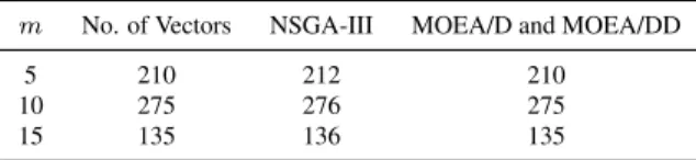
Table 1: Population size of three algorithmsm No. of Vectors NSGA-III MOEA/D and MOEA/DD
5 210 212 210
10 275 276 275
15 135 136 135
• SPEA2+SDE [27]: SPEA2+SDE incorporates shift-based density estima-tion into SPEA2 for MaOPs.
• MOEA/D [42]: Herein, MOEA/D with the penalty-based boundary inter-section (PBI) function is used in our experiments.
• NSGA-III [8]: NSGA-III is a reference-point-based MaOEA following the NSGA-II framework.
• MOMBI-II [16]:MOMBI-II is a recently proposed indicator-based MaOEA, which adopts theR2indicator as the selection criterion.
• MOEA/DD [26]: MOEA/DD is based on both Pareto dominance and de-composition.
• Two Arch2 [35]:Two Arch2 assigns different selection principles (indicator-based and Pareto-(indicator-based) to two archives for convergence and diversity, re-spectively.
4.4. Parameter Settings
• Population Size: Table 1 presents the population size of NSGA-III, MOEA/D, and MOEA/DD. For other algorithms, the population size was kept the same as NSGA-III.
• Parameter Settings for Evolutionary Operators: For all algorithms, SBX and the polynomial mutation were used to produce offspring. The crossover probability and the mutation probability were set to 1.0 and 1/n, respec-tively, and the distribution indexes of both SBX and the polynomial muta-tion were set to 20.
• Number of Independent Runs and Termination Condition: All algorithms were independently run 20 times on each test problem, and terminated when 90,000 function evaluations (FEs) were reached [35, 24].
ACCEPTED MANUSCRIPT
• Parameter Settings for Algorithms: For RVEA [4],α = 2andfr = 0.1for
all test problems following the suggestion in [4]. For MOEA/D [42], the neighborhood size was set to 20, the maximum replacement number was set to 2, and the penalty parameterθwas set to 5. For MOEA/DD [26], the
neighborhood size and θ were kept the same as MOEA/D, and the
proba-bility δ was set to 0.9. According to [16], two parameters in MOMBI-II
were set as= 0.001andα= 0.5, respectively.
In this paper, all the experiments were implemented in the platform recently developed by Tianet al.[31].
5. Results and Discussions 5.1. Benefit of Two Strategies
Firstly, we are interested in identifying the benefit of two crucial strategies of AnD: angle-based selection and shift-based density estimation. To this end, two variants of AnD were devised named AnD-WoA and AnD-WoD, respectively. In AnD-WoA, angle-based selection was eliminated. Instead, the individuals in the union population Ut were sorted based on their shift-based density values [25],
and N individuals with the highest density values were removed from Ut. In
AnD-WoD, shift-based density estimation was abandoned. As an alternative, for two individuals with the minimum vector angle, their Euclidean distances to the ideal point were computed, and the one with the larger Euclidean distance was deleted [11, 15]. The comparative experiments between AnD and its two variants were carried out on the DTLZ and WFG test suites. The IGD and HV values are shown in Table 2 and Table 3, respectively.
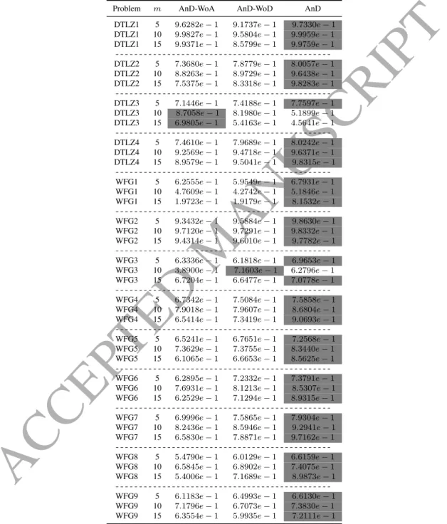
From Table 2 and Table 3, it is evident that AnD outperforms its two variants on a vast majority of test problems. In terms of the IGD metric, AnD obtains the best performance on 30 out of 39 test problems, while WoA and AnD-WoD achieve the best performance on only five and four test problems, respec-tively. With respect to the HV metric, AnD performs the best on 36 test problems. Nevertheless, AnD-WoA and AnD-WoD perform the best on no more than two test problems. The reason for the above results seems obvious. Compared with AnD, AnD-WoA discards angle-based selection, therefore it is unable to maintain the diversity of search directions. Regarding AnD-WoD, it replaces shift-based density estimation with the Euclidean distance. However, the Euclidean distance only considers an individual’s convergence property; thus, it is less reasonable
ACCEPTED MANUSCRIPT
Table 2: Performance comparison of AnD, AnD-WoA, and AnD-WoD in terms of the average IGD value on the DTLZ and WFG test suites. The best average IGD value among all the algorithms on each test problem is highlighted in Gray.Problem m AnD-WoA AnD-WoD AnD DTLZ1 5 7.1041e−2 7.3325e−2 6.0100e−2 DTLZ1 10 1.2443e−1 1.6631e−1 1.2504e−1 DTLZ1 15 1.7912e−1 2.3414e−1 1.9064e−1 DTLZ2 5 2.4507e−1 1.6893e−1 1.6826e−1 DTLZ2 10 4.8020e−1 4.5503e−1 3.7456e−1 DTLZ2 15 7.4842e−1 7.3188e−1 5.4876e−1 DTLZ3 5 2.5380e−1 1.9300e−1 1.8791e−1 DTLZ3 10 4.8583e−1 4.9184e−1 1.1336e+ 0 DTLZ3 15 7.6376e−1 9.1091e−1 1.8929e+ 0 DTLZ4 5 2.4661e−1 1.6692e−1 1.6868e−1 DTLZ4 10 4.5454e−1 4.0055e−1 3.7863e−1 DTLZ4 15 6.8081e−1 5.9132e−1 5.5382e−1 WFG1 5 9.3495e−1 1.0391e+ 0 8.2485e−1 WFG1 10 1.9120e+ 0 2.3222e+ 0 1.8344e+ 0 WFG1 15 4.2708e+ 0 4.4120e+ 0 2.5826e+ 0 WFG2 5 1.2924e+ 0 1.2482e+ 0 7.4199e−1 WFG2 10 4.8891e+ 0 4.6090e+ 0 3.7346e+ 0 WFG2 15 1.4048e+ 1 1.4005e+ 1 1.2394e+ 1 WFG3 5 1.0499e+ 0 8.2442e−1 5.0305e−1 WFG3 10 1.5811e+ 0 2.1080e+ 0 1.7025e+ 0 WFG3 15 8.6690e+ 0 1.2946e+ 0 2.6156e+ 0 WFG4 5 1.2669e+ 0 9.4798e−1 9.5061e−1 WFG4 10 4.6742e+ 0 4.3908e+ 0 3.6441e+ 0 WFG4 15 1.0007e+ 1 1.0596e+ 1 7.6264e+ 0 WFG5 5 1.2722e+ 0 9.5546e−1 9.3925e−1 WFG5 10 4.7402e+ 0 4.2061e+ 0 3.5788e+ 0 WFG5 15 1.0252e+ 1 9.4419e+ 0 7.5925e+ 0 WFG6 5 1.3676e+ 0 9.3884e−1 9.5995e−1 WFG6 10 4.7496e+ 0 4.0846e+ 0 3.5574e+ 0 WFG6 15 1.1015e+ 1 1.0492e+ 1 7.5193e+ 0 WFG7 5 1.3386e+ 0 9.5717e−1 9.5631e−1 WFG7 10 4.6176e+ 0 4.1528e+ 0 3.4909e+ 0 WFG7 15 1.0715e+ 1 9.7741e+ 0 7.5817e+ 0 WFG8 5 1.3795e+ 0 1.0943e+ 0 1.0138e+ 0 WFG8 10 5.4254e+ 0 5.0135e+ 0 3.8497e+ 0 WFG8 15 1.1483e+ 1 1.2461e+ 1 8.8015e+ 0 WFG9 5 1.2789e+ 0 1.0351e+ 0 9.4961e−1 WFG9 10 4.9261e+ 0 4.6810e+ 0 3.9489e+ 0 WFG9 15 1.0603e+ 1 9.8005e+ 0 8.0252e+ 0
ACCEPTED MANUSCRIPT
Table 3: Performance comparison of of AnD, AnD-WoA, and AnD-WoD in terms of the average HV value on the DTLZ and WFG test suites. The best average HV value among all the algorithms on each test problem is highlighted in Gray.Problem m AnD-WoA AnD-WoD AnD DTLZ1 5 9.6282e−1 9.1737e−1 9.7330e−1 DTLZ1 10 9.9827e−1 9.5804e−1 9.9959e−1 DTLZ1 15 9.9371e−1 8.5799e−1 9.9759e−1 DTLZ2 5 7.3680e−1 7.8779e−1 8.0057e−1 DTLZ2 10 8.8263e−1 8.9729e−1 9.6438e−1 DTLZ2 15 7.5375e−1 8.3318e−1 9.8283e−1 DTLZ3 5 7.1446e−1 7.4188e−1 7.7597e−1 DTLZ3 10 8.7058e−1 8.1980e−1 5.1899e−1 DTLZ3 15 6.9805e−1 5.4163e−1 4.5641e−1 DTLZ4 5 7.4610e−1 7.9689e−1 8.0242e−1 DTLZ4 10 9.2569e−1 9.4718e−1 9.6371e−1 DTLZ4 15 8.9579e−1 9.5041e−1 9.8315e−1 WFG1 5 6.2555e−1 5.9549e−1 6.7931e−1 WFG1 10 4.7609e−1 4.2742e−1 5.1846e−1 WFG1 15 1.9723e−1 1.9179e−1 8.1532e−1 WFG2 5 9.3432e−1 9.5884e−1 9.8630e−1 WFG2 10 9.7120e−1 9.7291e−1 9.8332e−1 WFG2 15 9.4314e−1 9.6010e−1 9.7782e−1 WFG3 5 6.3336e−1 6.1818e−1 6.9653e−1 WFG3 10 3.8900e−1 7.1603e−1 6.2796e−1 WFG3 15 6.7204e−1 6.6477e−1 7.0778e−1 WFG4 5 6.7342e−1 7.5084e−1 7.5858e−1 WFG4 10 7.9018e−1 7.9607e−1 8.6804e−1 WFG4 15 6.5414e−1 7.3419e−1 9.0693e−1 WFG5 5 6.5241e−1 6.7651e−1 7.2568e−1 WFG5 10 7.3629e−1 7.3755e−1 8.3440e−1 WFG5 15 6.1065e−1 6.6653e−1 8.5625e−1 WFG6 5 6.2895e−1 7.2332e−1 7.3791e−1 WFG6 10 7.6931e−1 8.1213e−1 8.5307e−1 WFG6 15 6.2529e−1 7.1294e−1 8.9315e−1 WFG7 5 6.9996e−1 7.5865e−1 7.9304e−1 WFG7 10 8.2436e−1 8.5946e−1 9.2941e−1 WFG7 15 6.5830e−1 7.8871e−1 9.7162e−1 WFG8 5 5.4790e−1 6.0129e−1 6.6159e−1 WFG8 10 6.5845e−1 6.8902e−1 7.4075e−1 WFG8 15 5.4006e−1 7.1689e−1 8.9873e−1 WFG9 5 6.1183e−1 6.4993e−1 6.6130e−1 WFG9 10 7.1796e−1 6.7073e−1 7.3830e−1 WFG9 15 6.3554e−1 5.9935e−1 7.2111e−1
ACCEPTED MANUSCRIPT
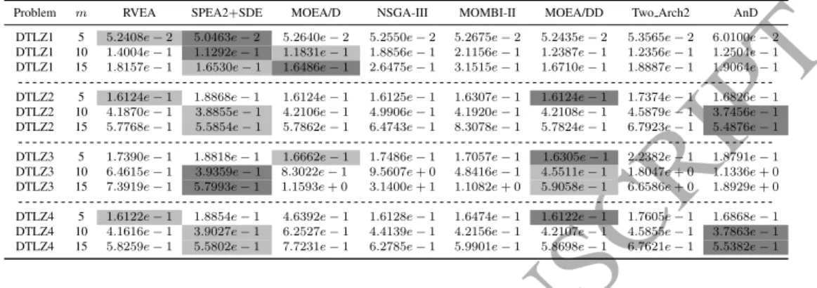
Table 4: Performance comparison between AnD and seven state-of-the-art MaOEAs in terms of the average IGD value on the DTLZ test suite. The best and second best average IGD values among all the algorithms on each test problem are highlighted in Gray and light Gray, respectively.Problem m RVEA SPEA2+SDE MOEA/D NSGA-III MOMBI-II MOEA/DD Two Arch2 AnD
DTLZ1 5 5.2408e−2 5.0463e−2 5.2640e−2 5.2550e−2 5.2675e−2 5.2435e−2 5.3565e−2 6.0100e−2 DTLZ1 10 1.4004e−1 1.1292e−1 1.1831e−1 1.8856e−1 2.1156e−1 1.2387e−1 1.2356e−1 1.2504e−1 DTLZ1 15 1.8157e−1 1.6530e−1 1.6486e−1 2.6475e−1 3.1515e−1 1.6710e−1 1.8887e−1 1.9064e−1 DTLZ2 5 1.6124e−1 1.8868e−1 1.6124e−1 1.6125e−1 1.6307e−1 1.6124e−1 1.7374e−1 1.6826e−1 DTLZ2 10 4.1870e−1 3.8855e−1 4.2106e−1 4.9906e−1 4.1920e−1 4.2108e−1 4.5879e−1 3.7456e−1 DTLZ2 15 5.7768e−1 5.5854e−1 5.7862e−1 6.4743e−1 8.3078e−1 5.7824e−1 6.7923e−1 5.4876e−1 DTLZ3 5 1.7390e−1 1.8818e−1 1.6662e−1 1.7486e−1 1.7057e−1 1.6305e−1 2.2382e−1 1.8791e−1 DTLZ3 10 6.4615e−1 3.9359e−1 8.3022e−1 9.5607e+ 0 4.8416e−1 4.5511e−1 1.8047e+ 0 1.1336e+ 0 DTLZ3 15 7.3919e−1 5.7993e−1 1.1593e+ 0 3.1400e+ 1 1.1082e+ 0 5.9058e−1 6.6586e+ 0 1.8929e+ 0 DTLZ4 5 1.6122e−1 1.8854e−1 4.6392e−1 1.6128e−1 1.6474e−1 1.6122e−1 1.7605e−1 1.6868e−1 DTLZ4 10 4.1616e−1 3.9027e−1 6.2527e−1 4.4139e−1 4.2156e−1 4.2107e−1 4.5855e−1 3.7863e−1 DTLZ4 15 5.8259e−1 5.5802e−1 7.7231e−1 6.2785e−1 5.9901e−1 5.8698e−1 6.7621e−1 5.5382e−1
Table 5: Performance comparison between AnD and seven state-of-the-art MaOEAs in terms of the average HV value on the DTLZ test suite. The best and second best average HV values among all the algorithms on each test problem are highlighted in Gray and light Gray, respectively.
Problem m RVEA SPEA2+SDE MOEA/D NSGA-III MOMBI-II MOEA/DD Two Arch2 AnD
DTLZ1 5 9.7971e−1 9.6924e−1 9.7942e−1 9.7962e−1 9.7942e−1 9.7977e−1 9.7582e−1 9.7330e−1 DTLZ1 10 9.9868e−1 9.9598e−1 9.9826e−1 9.1305e−1 9.6719e−1 9.9962e−1 9.9507e−1 9.9894e−1 DTLZ1 15 9.9950e−1 9.9122e−1 9.5880e−1 9.0076e−1 8.2655e−1 9.9707e−1 9.8287e−1 9.9759e−1 DTLZ2 5 8.1234e−1 8.1125e−1 8.1254e−1 8.1233e−1 8.1174e−1 8.1247e−1 7.6937e−1 8.0057e−1 DTLZ2 10 9.7440e−1 9.7222e−1 9.7529e−1 9.2862e−1 9.7439e−1 9.7531e−1 7.7695e−1 9.6438e−1 DTLZ2 15 9.8964e−1 9.8403e−1 9.8841e−1 9.3018e−1 8.4042e−1 9.9015e−1 6.3825e−1 9.8283e−1 DTLZ3 5 7.7880e−1 8.0874e−1 7.8499e−1 7.7721e−1 8.0386e−1 7.9779e−1 7.2701e−1 7.7597e−1 DTLZ3 10 7.0475e−1 9.6885e−1 4.9755e−1 0.0000e+ 0 9.3247e−1 9.2789e−1 1.6481e−1 5.1899e−1 DTLZ3 15 7.6387e−1 9.7532e−1 2.3293e−1 0.0000e+ 0 4.3883e−1 9.7556e−1 0.0000e+ 0 4.5641e−1 DTLZ4 5 8.1251e−1 8.1225e−1 6.6181e−1 8.1186e−1 8.1128e−1 8.1256e−1 7.5774e−1 8.0242e−1 DTLZ4 10 9.7383e−1 9.7124e−1 8.7615e−1 9.6258e−1 9.7453e−1 9.7536e−1 7.8132e−1 9.6371e−1 DTLZ4 15 9.8789e−1 9.8745e−1 8.8487e−1 9.5702e−1 9.8474e−1 9.8837e−1 6.3605e−1 9.8315e−1
than shift-based density estimation which takes both diversity and convergence into account.
From this discussion, we can conclude that angle-based selection and shift-based density estimation are two indispensable strategies in AnD.
5.2. Comparison with Seven State-of-the-Art MaOEAs
We compared the performance of AnD with that of the seven peer algorithms introduced in Section 4.3 on the DTLZ and WFG test suites in terms of the IGD and HV metrics. The results are summarized in Tables 4–7. At first glance, RVEA, SPEA2+SDE, and MOEA/DD achieve superior performance on the DTLZ test suite. The reason might be that the DTLZ test suite puts more emphasis on an al-gorithm’s convergence ability than its ability to diversity [20]. Note, however, that
ACCEPTED MANUSCRIPT
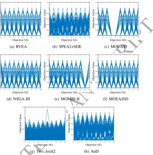
1 2 3 4 5 6 7 8 9 10 Objective NO. 0 0.1 0.2 0.3 0.4 0.5 0.6 Objective Value (a) RVEA 1 2 3 4 5 6 7 8 9 10 Objective NO. 0 0.1 0.2 0.3 0.4 0.5 0.6 Objective Value (b) SPEA2+SDE 1 2 3 4 5 6 7 8 9 10 Objective NO. 0 0.1 0.2 0.3 0.4 0.5 0.6 Objective Value (c) MOEA/D 1 2 3 4 5 6 7 8 9 10 Objective NO. 0 0.1 0.2 0.3 0.4 0.5 0.6 0.7 0.8 Objective Value (d) NSGA-III 1 2 3 4 5 6 7 8 9 10 Objective NO. 0 0.1 0.2 0.3 0.4 0.5 0.6 Objective Value (e) MOMBI-II 1 2 3 4 5 6 7 8 9 10 Objective NO. 0 0.1 0.2 0.3 0.4 0.5 0.6 Objective Value (f) MOEA/DD 1 2 3 4 5 6 7 8 9 10 Objective NO. 0 0.1 0.2 0.3 0.4 0.5 0.6 Objective Value (g) Two Arch2 1 2 3 4 5 6 7 8 9 10 Objective NO. 0 0.2 0.4 0.6 0.8 1 Objective Value (h) AnDFigure 4: The final solution sets of the eight compared algorithms on DTLZ1 with ten objectives by parallel coordinates.
AnD obtains the best overall performance on the WFG test suite. To visualize the results, we plotted the final populations resulting from the eight compared algori-thms in a typical run by parallel coordinates on four representative test problems in Figs. 4–7. Note that a typical run means a run producing the median IGD value among all runs. The detailed discussions are given next.
ACCEPTED MANUSCRIPT
1 2 3 4 5 6 7 8 9 10 Objective NO. 0 0.2 0.4 0.6 0.8 1 1.2 Objective Value (a) RVEA 1 2 3 4 5 6 7 8 9 10 Objective NO. 0 0.2 0.4 0.6 0.8 1 1.2 Objective Value (b) SPEA2+SDE 1 2 3 4 5 6 7 8 9 10 Objective NO. 0 0.2 0.4 0.6 0.8 1 1.2 Objective Value (c) MOEA/D 1 2 3 4 5 6 7 8 9 10 Objective NO. 0 0.2 0.4 0.6 0.8 1 1.2 Objective Value (d) NSGA-III 1 2 3 4 5 6 7 8 9 10 Objective NO. 0 0.2 0.4 0.6 0.8 1 1.2 Objective Value (e) MOMBI-II 1 2 3 4 5 6 7 8 9 10 Objective NO. 0 0.2 0.4 0.6 0.8 1 1.2 Objective Value (f) MOEA/DD 1 2 3 4 5 6 7 8 9 10 Objective NO. 0 0.5 1 1.5 Objective Value (g) Two Arch2 1 2 3 4 5 6 7 8 9 10 Objective NO. 0 0.2 0.4 0.6 0.8 1 1.2 Objective Value (h) AnDFigure 5: The final solution sets of the eight compared algorithms on DTLZ4 with ten objectives by parallel coordinates.
5.2.1. DTLZ Test Suite
From Tables 4 and 5, we observe that the eight compared algorithms exhibit mixed performance. More specifically, SPEA2+SDE performs the best in terms of the IGD metric, followed by MOEA/DD and AnD, as shown in Table 4. Never-theless, MOEA/DD and RVEA obtain the best and second best performance with respect to the HV metric, respectively, as shown in Table 5.
ACCEPTED MANUSCRIPT
DTLZ1 is a multimodal problem, in which the PF is degenerate and the de-cision variables are non-separable. It challenges the convergence performance of an algorithm. We find that SPEA2+SDE achieves the best IGD values on five and 10 objectives, while MOEA/D obtains the best IGD value on 15 ob-jectives. As far as HV is concerned, MOEA/DD outperforms the others on five and 10 objectives, and RVEA beats its competitors on 15 objectives. As shown in Fig. 4, the results provided by some methods using weight vectors or reference points (i.e., MOEA/D and MOEA/DD) have better distributions. With respect to SPEA2+SDE and Two Arch2, the scales of some objective values are smaller than the true PF, which suggests that they have a preference on the solutions lo-cated in central areas. In terms of AnD, some extreme values for the third, fourth, and sixth objectives occur, which means that AnD has relatively poor convergence performance on DTLZ1.
DTLZ2 is a relatively simple test problem compared with DTLZ1, which is mainly used to test an algorithm’s diversity. AnD achieves the best overall IGD performance, while MOEA/DD obtains the best overall HV performance. In AnD, the diversity of the population is considered in both angle-based selection and shift-based density estimation; therefore, AnD provides promising results on DTLZ2.
For DTLZ3, which is a highly multimodal problem, SPEA2+SDE achieves the best overall performance in terms of both IGD and HV. From Table 5, it can be seen that the results provided by NSGA-III and Two Arch2 are distant from the PFs on 10 and 15 objectives. AnD obtains medium performance in terms of both IGD and HV.
Regarding DTLZ4, the density of points on its PF is strongly biased. There-fore, the main challenge for solving this test problem is to maintain the diversity of the population. Similar to DTLZ2, AnD and MOEA/DD obtain the best over-all IGD and HV performance, respectively. From Fig. 5, it can be observed that Two Arch2 produces some extreme values on the sixth objective, which suggests unstable convergence performance. The results obtained by RVEA, NSGA-III, and MOEA/DD distribute similarly and concentrate mainly on the boundary or the middle parts of the PF. As for MOEA/D, its results fail to cover the fourth and fifth objectives well. Similarly, the results obtained by MOMBI-II are unable to cover the ninth objective well. SPEA2+SDE and AnD are capable of covering the whole PF. The difference between them is that the objective values derived from SPEA2+SDE mainly lie in [0, 0.8], while in AnD, they are well distributed within [0, 1].
ACCEPTED MANUSCRIPT
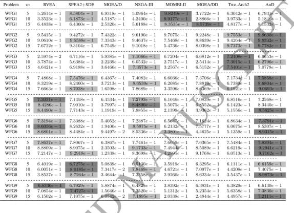
Table 6: Performance comparison between AnD and seven state-of-the-art MaOEAs in terms of the average IGD value on the WFG test suite. The best and second best average IGD values among all the algorithms on each test problem are highlighted in Gray and light Gray, respectively.Problem m RVEA SPEA2+SDE MOEA/D NSGA-III MOMBI-II MOEA/DD Two Arch2 AnD
WFG1 5 1.2380e+ 0 4.5051e−1 1.4719e+ 0 1.3003e+ 0 7.3247e−1 1.7863e+ 0 9.5226e−1 8.2485e−1 WFG1 10 2.4159e+ 0 1.5483e+ 0 3.5093e+ 0 2.3319e+ 0 2.9849e+ 0 2.7158e+ 0 2.2678e+ 0 1.8344e+ 0 WFG1 15 3.4128e+ 0 3.0000e+ 0 5.4507e+ 0 3.6069e+ 0 6.0947e+ 0 4.2376e+ 0 3.1632e+ 0 2.5826e+ 0 WFG2 5 7.3061e−1 9.9429e−1 2.9028e+ 0 6.2450e−1 1.2746e+ 0 1.9358e+ 0 4.7796e−1 7.4199e−1 WFG2 10 3.6478e+ 0 5.4046e+ 0 1.1021e+ 1 4.0066e+ 0 3.9907e+ 0 1.1009e+ 1 1.9916e+ 0 3.7346e+ 0 WFG2 15 1.2716e+ 1 1.4549e+ 1 1.6855e+ 1 1.2405e+ 1 1.9653e+ 1 1.5737e+ 1 5.7470e+ 0 1.2394e+ 1 WFG3 5 6.4564e−1 5.8114e−1 1.0504e+ 0 4.7212e−1 9.5483e−1 6.5805e−1 3.6891e−1 5.0305e−1 WFG3 10 3.0551e+ 0 1.7028e+ 0 8.6850e+ 0 8.7259e−1 9.3633e+ 0 2.8279e+ 0 1.2887e+ 0 1.7025e+ 0 WFG3 15 6.2924e+ 0 4.5129e+ 0 1.6375e+ 1 3.2111e+ 0 1.6002e+ 1 1.4214e+ 1 2.5444e+ 0 2.6156e+ 0 WFG4 5 9.4475e−1 1.1148e+ 0 1.6793e+ 0 9.5187e−1 1.7483e+ 0 1.0314e+ 0 9.7618e−1 9.5061e−1 WFG4 10 3.8034e+ 0 4.1323e+ 0 8.9303e+ 0 4.0807e+ 0 8.3168e+ 0 5.2137e+ 0 4.5821e+ 0 3.6441e+ 0 WFG4 15 8.7523e+ 0 8.2858e+ 0 1.6011e+ 1 8.9661e+ 0 2.3009e+ 1 9.1948e+ 0 9.7013e+ 0 7.6264e+ 0 WFG5 5 9.3668e−1 1.1233e+ 0 1.5112e+ 0 9.3688e−1 1.6929e+ 0 1.0146e+ 0 9.7161e−1 9.3925e−1 WFG5 10 3.8534e+ 0 4.0242e+ 0 8.6325e+ 0 3.8863e+ 0 7.2474e+ 0 5.9057e+ 0 4.5803e+ 0 3.5788e+ 0 WFG5 15 8.2300e+ 0 1.0363e+ 1 1.6180e+ 1 8.6808e+ 0 2.7050e+ 1 1.3822e+ 1 9.6726e+ 0 7.5925e+ 0 WFG6 5 9.4927e−1 1.1683e+ 04 1.9082e+ 0 9.5167e−1 1.6161e+ 0 1.0294e+ 0 9.8289e−1 9.5995e−1 WFG6 10 3.8553e+ 0 4.1209e+ 0 9.7139e+ 0 3.9288e+ 0 7.5219e+ 0 5.4913e+ 0 4.5845e+ 0 3.5574e+ 0 WFG6 15 8.5768e+ 0 9.3893e+ 0 1.6228e+ 1 9.0585e+ 0 2.3092e+ 1 1.3704e+ 1 9.7084e+ 0 7.5193e+ 0 WFG7 5 9.5376e−1 1.1481e+ 0 1.7551e+ 0 9.5434e−1 1.4084e+ 0 1.0384e+ 0 9.5596e−1 9.5631e−1 WFG7 10 3.8105e+ 0 3.9180e+ 0 9.6364e+ 0 4.1474e+ 0 7.0575e+ 0 4.8005e+ 0 4.5546e+ 0 3.4909e+ 0 WFG7 15 8.4477e+ 0 8.1509e+ 0 1.6400e+ 1 9.2815e+ 0 2.2087e+ 1 8.0829e+ 0 9.9669e+ 0 7.5817e+ 0 WFG8 5 9.8533e−1 1.1560e+ 0 1.2965e+ 0 1.0084e+ 0 2.3995e+ 0 1.0543e+ 0 1.1102e+ 0 1.0138e+ 0 WFG8 10 3.9040e+ 0 4.3343e+ 0 8.1439e+ 0 5.1141e+ 0 8.8767e+ 0 4.1808e+ 0 5.4467e+ 0 3.8497e+ 0 WFG8 15 9.5526e+ 0 8.5588e+ 0 1.2660e+ 1 1.0520e+ 1 2.3945e+ 1 9.0171e+ 0 1.0866e+ 1 8.8015e+ 0 WFG9 5 9.1032e−1 1.0663e+ 0 1.3802e+ 0 9.2301e−1 2.2015e+ 0 1.0173e+ 0 1.0066e+ 0 9.4961e−1 WFG9 10 4.1319e+ 0 4.2572e+ 0 9.0024e+ 0 4.1250e+ 0 6.7789e+ 0 6.0132e+ 0 5.1443e+ 0 3.9489e+ 0 WFG9 15 8.2901e+ 0 9.1482e+ 0 1.5257e+ 1 8.6989e+ 0 2.7200e+ 1 1.2606e+ 1 1.0647e+ 1 8.0252e+ 0 5.2.2. WFG Test Suite
The first observation from Tables 6 and 7 is that AnD attains the best overall performance in terms of both IGD and HV. Next, we give the detailed discussions. Table 6 shows the IGD values resulting from the eight compared algorithms. Clearly, AnD and RVEA are the two top algorithms, and they have a clear ad-vantage over the other six algorithms on the majority of test problems. Actually, AnD provides the best and second best IGD values on 12 and six out of 27 test problems, respectively. As for RVEA, it generates six best results and nine second best results. In addition, SPEA2+SDE obtains three best results and two second best results, Two Arch2 produces five best results, NSGA-III has one best result and seven second best results, and MOEA/DD and MOMBI-II reach one sec-ond best result each. One interesting phenomenon we have observed is that the methods based on weight vectors or reference points (i.e., MOEA/D, MOEA/DD, NSGA-III, and MOMBI-II) seem to lose their effectiveness on this test suite. This
ACCEPTED MANUSCRIPT
Table 7: Performance comparison between AnD and seven state-of-the-art MaOEAs in terms of the average HV value on the WFG test suite. The best and second best average HV values among all the algorithms on each test problem are highlighted in Gray and light Gray, respectively.Problem m RVEA SPEA2+SDE MOEA/D NSGA-III MOMBI-II MOEA/DD Two Arch2 AnD
WFG1 5 5.2614e−1 8.5804e−1 6.9318e−1 5.0964e−1 9.8249e−1 3.7722e−1 6.3042e−1 6.7931e−1 WFG1 10 3.3523e−1 6.1873e−1 4.5187e−1 4.2400e−1 9.9177e−1 2.8866e−1 3.9733e−1 5.1846e−1 WFG1 15 6.4838e−1 6.4360e−1 2.5320e−1 5.6188e−1 8.3535e−1 8.5739e−1 4.8177e−1 8.1532e−1 WFG2 5 9.5415e−1 9.4272e−1 7.4322e−1 9.6190e−1 9.7075e−1 9.2248e−1 9.7553e−1 9.8630e−1 WFG2 10 9.0610e−1 9.5588e−1 7.3343e−1 9.4637e−1 7.5468e−1 8.8639e−1 9.4264e−1 9.8332e−1 WFG2 15 7.6722e−1 9.3104e−1 6.7549e−1 9.1018e−1 5.4736e−1 8.0398e−1 9.7373e−1 9.7782e−1 WFG3 5 2.5974e−2 6.7116e−1 5.9385e−1 7.1066e−1 6.7204e−1 6.6812e−1 7.2408e−1 6.9653e−1 WFG3 10 3.7874e−1 5.6384e−1 2.2239e−1 6.0532e−1 2.7517e−1 2.5414e−1 7.3015e−1 6.2796e−1 WFG3 15 4.6421e−1 6.9188e−1 3.6466e−1 7.3573e−1 3.2567e−1 6.5152e−1 7.5401e−1 7.0778e−1 WFG4 5 7.4868e−1 7.5476e−1 6.4367e−1 7.4082e−1 6.6036e−1 7.3706e−1 7.1734e−1 7.5858e−1 WFG4 10 8.3259e−1 8.2460e−1 3.7213e−1 8.6530e−1 6.2085e−1 7.8810e−1 6.7389e−1 8.6804e−1 WFG4 15 7.6663e−1 8.7028e−1 1.6598e−1 7.8689e−1 3.3596e−1 8.6369e−1 6.1921e−1 9.0693e−1 WFG5 5 7.3031e−1 7.1458e−1 6.4534e−1 7.2793e−1 6.1046e−1 7.0839e−1 6.8516e−1 7.2568e−1 WFG5 10 8.4286e−1 7.9010e−1 3.7997e−1 8.4800e−1 5.5075e−1 6.8552e−1 6.1423e−1 8.3440e−1 WFG5 15 8.4490e−1 7.7143e−1 1.1919e−1 7.8855e−1 2.1399e−1 3.9362e−1 5.1556e−1 8.5625e−1 WFG6 5 7.3194e−1 7.3388e−1 5.4052e−1 7.2387e−1 6.5647e−1 7.1624e−1 6.8634e−1 7.3791e−1 WFG6 10 8.6056e−1 8.2632e−1 1.9400e−1 8.5875e−1 6.2132e−1 7.5777e−1 6.0675e−1 8.5307e−1 WFG6 15 8.6801e−1 8.4484e−1 9.4497e−2 8.5336e−1 3.3801e−1 4.4625e−1 5.1359e−1 8.9315e−1 WFG7 5 7.8637e−1 7.8067e−1 6.3867e−1 7.7461e−1 7.6659e−1 7.6365e−1 7.5484e−1 7.9304e−1 WFG7 10 8.8809e−1 8.9075e−1 2.3503e−1 9.1733e−1 7.4944e−1 8.5089e−1 6.6219e−1 9.2941e−1 WFG7 15 7.2147e−1 9.2918e−1 1.2338e−1 8.3698e−1 4.2995e−1 9.1768e−1 6.0513e−1 9.7162e−1 WFG8 5 6.4019e−1 6.7275e−1 5.0839e−1 6.5130e−1 3.5919e−1 6.3295e−1 6.1111e−1 6.6159e−1 WFG8 10 6.0051e−1 8.0185e−1 7.3417e−2 7.8469e−1 4.6721e−1 7.0977e−1 4.4208e−1 7.4075e−1 WFG8 15 3.8537e−1 8.7264e−1 3.4644e−1 7.3358e−1 2.9260e−1 8.6234e−1 3.5437e−1 8.9873e−1 WFG9 5 6.8336e−1 6.7929e−1 5.8874e−1 6.4825e−1 3.8392e−1 6.3831e−1 6.3829e−1 6.6130e−1 WFG9 10 7.0854e−1 7.4727e−1 1.5646e−1 7.3520e−1 5.1312e−1 5.2354e−1 5.6358e−1 7.3830e−1 WFG9 15 6.1502e−1 7.1075e−1 6.0542e−2 7.1895e−1 2.0338e−1 2.4844e−1 4.4957e−1 7.2111e−1
can be attributed to the fact that the PFs of the WFG test suite are irregular, dis-continued or mixed, and scaled with different ranges in each objective. Therefore, well-distributed weight vectors/reference points cannot guarantee a good distri-bution of the obtained solutions. Note, however, that RVEA, which also uses the reference vectors to guide the search, performs better than MOEA/D, MOEA/DD, NSGA-III, and MOMBI-II. This is perhaps because the use of angle information helps RVEA to alleviate this issue to a certain degree.
The HV values are given in Table 7. From Table 7, AnD and SPEA2+SDE achieve the best and second best overall performance, respectively. Specifically, AnD produces 14 best results and three second best results out of 27 test pro-blems, and SPEA2+SDE has three best results and eight second best results. It is also observed that AnD reaches the best performance on WFG2, WFG4, WFG6, and WFG7. For MOMBI-II, Two Arch2, RVEA, and SPEA2+SDE, they exhibit the best overall performance on WFG1, WFG3, WFG5, and WFG8, respectively.
ACCEPTED MANUSCRIPT
1 2 3 4 5 6 7 8 9 10 Objective NO. 0 5 10 15 20 25 Objective Value (a) RVEA 1 2 3 4 5 6 7 8 9 10 Objective NO. 0 5 10 15 20 25 Objective Value (b) SPEA2+SDE 1 2 3 4 5 6 7 8 9 10 Objective NO. 0 1 2 3 4 5 6 Objective Value (c) MOEA/D 1 2 3 4 5 6 7 8 9 10 Objective NO. 0 5 10 15 20 25 Objective Value (d) NSGA-III 1 2 3 4 5 6 7 8 9 10 Objective NO. 0 5 10 15 20 25 Objective Value (e) MOMBI-II 1 2 3 4 5 6 7 8 9 10 Objective NO. 0 5 10 15 20 25 Objective Value (f) MOEA/DD 1 2 3 4 5 6 7 8 9 10 Objective NO. 0 5 10 15 20 25 Objective Value (g) Two Arch2 1 2 3 4 5 6 7 8 9 10 Objective NO. 0 5 10 15 20 25 Objective Value (h) AnDFigure 6: The final solution sets of the eight compared algorithms on WFG4 with ten objectives by parallel coordinates.
With regard to WFG9, AnD and SPEA2+SDE are the two best algorithms. With the aim of revealing more details of the eight compared algorithms, their results on both WFG4 and WFG7 with ten objectives are presented by parallel coordinates in Figs. 6 and 7, respectively. From Fig. 6, one can see that MOEA/D and MOEA/DD have relatively poor distributions. It might be because they lack a normalization procedure before the evaluation of an individual. As for RVEA and MOMBI-II, the former fails to cover the seventh objective well, while the latter is
ACCEPTED MANUSCRIPT
1 2 3 4 5 6 7 8 9 10 Objective NO. 0 5 10 15 20 25 Objective Value (a) RVEA 1 2 3 4 5 6 7 8 9 10 Objective NO. 0 5 10 15 20 25 Objective Value (b) SPEA2+SDE 1 2 3 4 5 6 7 8 9 10 Objective NO. 0 0.5 1 1.5 2 2.5 3 3.5 Objective Value (c) MOEA/D 1 2 3 4 5 6 7 8 9 10 Objective NO. 0 5 10 15 20 25 Objective Value (d) NSGA-III 1 2 3 4 5 6 7 8 9 10 Objective NO. 0 5 10 15 20 25 Objective Value (e) MOMBI-II 1 2 3 4 5 6 7 8 9 10 Objective NO. 0 5 10 15 20 25 Objective Value (f) MOEA/DD 1 2 3 4 5 6 7 8 9 10 Objective NO. 0 5 10 15 20 25 Objective Value (g) Two Arch2 1 2 3 4 5 6 7 8 9 10 Objective NO. 0 5 10 15 20 25 Objective Value (h) AnDFigure 7: The final solution sets of the eight compared algorithms on WFG7 with ten objectives by parallel coordinates.
unable to cover the first four objectives well. In terms of SPEA2+SDE, NSGA-III, Two Arch2, and AnD, all of them can cover the whole PF. The difference between them is that the results derived from SPEA2+SDE, NSGA-III, and Two Arch2 concentrate mainly on the boundary or the middle parts of the PF, while in AnD, the results can spread out the whole PF very well. A similar phenomena can also be observed in Fig. 7. AnD still has the best distribution. Note that NSGA-III fails to cover the first objective well.
ACCEPTED MANUSCRIPT
0 5 10 15 20 25 30 35 better similar worse Num ber of Test Probl em s (a) IGD 0 5 10 15 20 25 30 35 40 better similar worse N um ber of Test Problem s (b) HVFigure 8: Wilcoxon rank-sum test between AnD and its seven competitors (i.e., RVEA, SPEA2+SDE, MOEA/D, NSGA-III, MOMBI-II, MOEA/DD, and Two Arch2) on all the test pro-blems (including the DTLZ and WFG test suites) in terms of IGD and HV. “better“, “similar“ and “worse“ mean that a competitor performs better than, similar to, and worse than AnD, respectively.
5.2.3. Discussion
To analyze the overall performance on both the DTLZ and WFG test suites, the Wilcoxon rank-sum test was implemented between AnD and the other seven MaOEAs in terms of both the IGD and HV metrics. The statistical test results are presented in Fig. 8. Fig. 8(a) gives the comparison results in terms of IGD. From Fig. 8(a), we can see that AnD outperforms RVEA, SPEA2+SDE, MOEA/D, NSGA-III, MOMBI-II, MOEA/DD, and Two Arch2 on 21, 29, 31, 23, 31, 29, and 29 test problems, respectively, while it loses on 10, eight, five, nine, six, eight, and seven test problems. The comparison results for HV are shown in Fig. 8(b). As shown in Fig. 8(b), AnD performs better than RAVE, SPEA2+SDE, MOEA/D, NSGA-III, MOMBI-II, MOEA/DD, and Two Arch2 on 22, 17, 31, 19, 26, 24, and 35 test problems, respectively, but performs worse on 14, 14, five, eight, 11, 12, and four test problems. Thus, we can conclude that AnD is able to obtain better overall performance compared with the seven competitors in terms of both IGD and HV.
Furthermore, the Friedman test was also implemented on all the test problems in terms of both IGD and HV. In the Friedman test, the smaller the ranking, the better the performance of the algorithm. From Fig. 9, it is evident that AnD has the smallest ranking in terms of both IGD and HV, followed by RVEA and SPEA2+SDE. RVEA ranks the third and second best in terms of IGD and HV, respectively. SPEA2+SDE works the second and third best in terms of IGD and
ACCEPTED MANUSCRIPT
3.0235 3.7051 6.6026 4.0256 6.5769 4.6923 4.6923 2.7308 0 1 2 3 4 5 6 7 Average Rank in g of th e Fri edm an Test (a) IGD 3.5897 3.2692 6.6154 4.0897 5.5897 4.2436 5.7179 2.8846 0 1 2 3 4 5 6 7 Av erage Rank in g o f th e Fried m an Test (b) HVFigure 9: Friedman test between AnD and its seven competitors (i.e., RVEA, SPEA2+SDE, MOEA/D, NSGA-III, MOMBI-II, MOEA/DD, and Two Arch2) on all the test problems (includ-ing the DTLZ and WFG test suites) in terms of IGD and HV. The smaller the rank(includ-ing, the better the performance of an algorithm.
HV, respectively. Theses results indicate that the algorithm with either shift-based density estimation (i.e., SPEA2+SDE) or angle information (i.e., RVEA) is more suitable for solving MaOPs. Moreover, the algorithm with these two elements (i.e., AnD) achieves the best performance, which verifies the main motivation of this paper.
5.3. Constrained MaOPs
One may be interested in whether AnD can be applied to solve constrained MaOPs, which are frequently encountered in real-world applications. To answer this question, AnD was extended to cope with this kind of optimization problem, and the resultant algorithm is called C-AnD.
The constraint-handling technique of C-AnD is inspired by the feasibility rule [7], which is a well-known constraint-handling technique for constrained single-objective optimization problems. Firstly, we compute the degree of con-straint violation for each individual:
CV(x) = J X j=1 max{0, gj(x)}+ K X k=1 |hk(x)|. (8)
wheregj ≥0andhj = 0denote thejth inequality constraint and thejth equality
constraint, respectively, andJ andKare the number of inequality constraints and equality constraints, respectively. Subsequently, the number of feasible solutions
ACCEPTED MANUSCRIPT
Table 8: Mean and standard deviation of the IGD and HV values on C1-DTLZ1, C2-DTLZ2, and C3-DTLZ4. The better result between C-AnD and C-NSGA-III on each test problem is highlighted in Gray.IGD m C-NSGA-III C-AnD
C1-DTLZ1 5 5.8093e−2(5.60e−3) 5.4026e−2(5.46e−3) C1-DTLZ1 10 1.2436e−1(4.98e−3) 1.1237e−1(3.26e−3) C1-DTLZ1 15 2.0774e−1(1.13e−2) 1.7216e−1(2.01e−3) C2-DTLZ2 5 1.8916e−1(7.44e−2) 1.5010e−1(6.73e−3) C2-DTLZ2 10 3.7888e−1(1.20e−1) 2.6826e−1(5.60e−2) C2-DTLZ2 15 7.2215e−1(1.56e−1) 2.6633e−1(1.62e−1) C3-DTLZ4 5 2.8139e−1(2.04e−2) 2.8605e−1(1.40e−2) C3-DTLZ4 10 5.7678e−1(6.60e−2) 5.4039e−1(1.34e−2) C3-DTLZ4 15 1.1089e+ 0(2.72e−1) 7.3981e−1(2.88e−3) HV m C-NSGA-III C-AnD C1-DTLZ1 5 9.7255e−1(2.73e−3) 9.7770e−1(1.90e−3) C1-DTLZ1 10 9.8800e−1(1.05e−2) 9.8803e−1(1.66e−2) C1-DTLZ1 15 9.5938e−1(3.76e−2) 9.9054e−1(1.19e−2) C2-DTLZ2 5 7.3902e−1(4.53e−2) 7.4493e−1(3.45e−3) C2-DTLZ2 10 8.3045e−1(7.04e−2) 8.7759e−1(1.46e−2) C2-DTLZ2 15 5.9223e−1(2.35e−1) 9.0674e−1(1.65e−1) C3-DTLZ4 5 9.4462e−1(2.68e−2) 9.5475e−1(1.61e−3) C3-DTLZ4 10 9.9877e−1(2.51e−3) 9.9909e−1(1.08e−4) C3-DTLZ4 15 9.5658e−1(3.70e−2) 9.9991e−1(1.84e−5)
in the union population Ut is calculated. If the number of feasible solutions is
larger thanN, thenAlgorithm 2is triggered to selectNfeasible solutions for the next generation from all the feasible solutions. Otherwise, we sort the individuals inUt according to their degree of constraint violations, and then chooseN
indi-viduals with the smallest degree of constraint violations for the next generation. Overall, the implementation of C-AnD is simple. The performance of C-AnD was compared with that of C-NSGA-III [21], which is the constrained version of NSGA-III, on three representative constrained MaOPs, namely C1-DTLZ1, C2-DTLZ2, and C3-DTLZ4 with five, 10, and 15 objectives. Both C-AnD and C-NSGA-III were run 20 times independently for each test problem. In each run, the maximum number of FEs was set to 180,000 for C1-DTLZ1, and 90,000 for C2-DTLZ2 and C3-DTLZ4. The results are summarized in Table 8.
From Table 8, it can be seen that C-AnD beats C-NSGA-III on all the test problems except C3-DTLZ4 with five objectives in terms of IGD. Therefore, C-AnD is also a simple and effective algorithm for constrained many-objective op-timization. It is worth noting that there are no reference points in C-AnD; thus