Scalarizing Functions in Bayesian Multiobjective Optimization

(1)

Scalarizing Functions in Bayesian Multiobjective

Optimization

Tinkle Chugh

Department of Computer Science, University of Exeter, UK

Abstract—Scalarizing functions have been widely used to con-vert a multiobjective optimization problem into a single objective optimization problem. However, their use in solving computation-ally expensive multi- and many-objective optimization problems using Bayesian multiobjective optimization is scarce. Scalarizing functions can play a crucial role on the quality and number of evaluations required when doing the optimization. In this article, we compare 15 different scalarizing functions in the framework of Bayesian multiobjective optimization and build Gaussian process models on them. We use the expected improvement as infill criterion (or acquisition function) to update the models. In particular, we analyze the performance of different scalarizing functions on several benchmark problems with different number of objectives to be optimized. The review and experiments on different functions provide useful insights in using a scalarizing function, especially for problems with a large number of objec-tives.

Index Terms—Pareto optimality, evolutionary multiobjective optimization, surrogate, metamodel

I. INTRODUCTION

Many real-world optimization problems have multiple con-flicting objectives to be achieved and use black-box computa-tionally expensive simulators. Surrogate-assisted optimization methods have been widely used in the literature to solve such problems. Many of these methods use Bayesian optimization involving Gaussian processes (or Kriging) as surrogate models. The Gaussian processes provide an advantage over other types of surrogate models because of their ability to provide uncertainty in predictions. For more details about surrogate-assisted methods, see e.g. surveys [1], [2], [3], [4], [5].

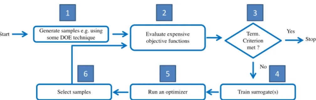
A generic framework of a Bayesian optimization method is shown in Figure 1. In the first step, a set of samples is generated e.g. using a design of experiment technique like Latin hypercube sampling [6]. In the second step, these samples are then evaluated with expensive objectives. In the third step, a termination criterion is checked. If the termination criterion is met, nondominated solutions from all expensive evaluated solutions are used as the final solutions. Otherwise, surrogate models are built using evaluated solutions in the fourth step. An optimizer e.g. an evolutionary algorithm is then used with the models in the fifth step to find promising samples by using an appropriate infilling criterion (or updating criterion or acquisition function). In the sixth step, a fixed number of samples generated with the optimizer is selected which are then evaluated with expensive objective functions.

All six steps mentioned above are important in the per-formance of a Bayesian optimization method [7]. In this

article, our focus is on the fourth step i.e. building or training surrogates. Once, the samples are evaluated with expensive objective functions in the second step, there can be different ways to build surrogates. The most common way is to build surrogate for each objective function [8], [9], [10]. Another way is to build a surrogate for a scalarizing function after converting multiobjective optimization problem into a single objective optimization problem [11], [12], which is also the focus of this article. There are other approaches for building surrogates like the classification of solutions into different ranks or classes [13], [14], [15]. For details on other ways of building surrogates, see [1], [3], [16]. Note that a scalarizing function can also be used after building models on each objective function e.g. as in [10] to do a local search. In this article, we focus on building surrogate after converting a multiobjective optimization problem into a single objective by using a scalarizing function.

There are two main advantages in using a single surrogate when solving an expensive MOP. The first one is that only one surrogate is used in the solution process instead of multiple surrogates, which reduces the computational burden e.g. the training time especially in many-objective (usually more than three objectives) optimization problems. The second advantage is that one can use an infill criterion proposed for single-objective optimization problems which also reduces the com-putational complexity. In the literature, a little attention has been paid in using scalarizing functions for building surrogates on them and only a few studies exist in the literature. For instance, in [11], an augmented achievement scalarizing func-tion (AASF) was used and in [12], hypervolume improvement, dominance rank and minimum signed distance were used (more details are provided in the Section III).

It is worth important to be pointed out that several studies exist [17], [18], [19], [20], [21] on using scalarizing functions without using them in a Bayesian optimization method. In this article, we study 15 different scalarizing functions and build surrogates on them in solving (computationally) expensive MOPs and particularly, focus on answering the following research questions:

1) are different scalarizing functions perform different to each other under the same framework?

2) are surrogate models built on a given scalarizing function sensitive to the number of objectives ?

(2)

scalar-Start Generate samples e.g. using some DOE technique

Select samples Run an optimizer

Term. Criterion

met ? Evaluate expensive

objective functions Stop

Train surrogate(s) Yes No 1 2 3 4 5 6

Fig. 1: A generic framework for a surrogate-assisted optimization method

izing functions into the framework of efficient global opti-mization (EGO) [22]. The algorithm uses the expected im-provement criterion for updating the surrogates build on the scalarizing function. We then test the method with different scalarizing functions on several benchmark problems with different numbers of objectives. We analyze the accuracy and uncertainty provided by Gaussian process models on different scalarizing functions with a different number of objectives.

The rest of the article is organized as follows. In the next section, we provide a literature survey on using scalarizing functions with and without building surrogates on them. In Section 3, we give a brief introduction to different functions with their mathematical formulations and merits and demerits. In Section 4, numerical experiments are conducted to answer the research questions mentioned above. We finally conclude and mention the future research directions in Section 5.

II. RELATEDWORK

Scalarizing functions have been used since decades in the Multiple Criteria Decision Making (MCDM) community [20], [21], [23], [24]. In evolutionary multiobjective optimization (EMO) algorithms especially decomposition based, utilization of scalarizing functions became popular in the last few years. Many studies and algorithms exist in the literature utilizing different functions for solving multi- and many-objectives op-timization problems. Some of the well-known decomposition based EMO algorithms utilizing different scalarizing func-tions are nondominated-sorting genetic algorithm III (NSGA-III) [25], multiobjective optimization based on decomposi-tion (MOEA/D) [26] and its numerous versions [27] and reference vector guided evolutionary algorithm (RVEA) [28]. For more details on the working principle of decomposition based algorithms, see surveys on many-objective optimization evolutionary algorithms [29], [30].

In [31], two different scalarizing functions weighted sum and augmented Chebyshev were used adaptively in the solu-tion process in the framework of MOEA/D by using a multi-grid scheme. The proposed idea was tested on a knapsack problem with four and six objectives and performed better than the original version of MOEA/D. The authors extended their work in [32], and modified the penalty boundary intersection (PBI) function in MOEA/D to handle different kinds of Pareto fronts. Two modified PBI functions called two-level PBI and

quadratic PBI were tested in the MOEA/D framework and the algorithm with two new scalarizing functions performed better than the original version.

A detailed study on different scalarizing functions and their corresponding parameters was conducted in [33]. Instead of proposing a new algorithm, the authors showed the per-formance of the different scalarizing functions in a simple (1+λ)-evolutionary algorithm [33] on bi-objective optimization problems. In [17], the performance of 15 different scalarizing functions was tested in MOEA/D [26] and MOMBI-II [34] algorithms. The authors used a tool called EVOCA [35] to tune the parameter values in different functions. Two algorithms MOEA/D and MOMBI-II [34] with different scalarizing func-tions were tested on Lame Supersphere test problems [36]. The authors found out that the performance of two algorithms depends on the choice of scalarizing functions.

In [19], a hyper-heuristic was used to rank different scalar-izing functions with a measure called s-energy [37]. The proposed algorithm was tested on ZDT, DTLZ and WFG benchmark problems with 2-10 objectives and compared with MOMBI-II, MOEA/D and NSGA-III and found better re-sults in most of the instances. In [38], two new scalarizing functions called the multiplicative scalarizing function (MSF) and penalty-based scalarizing function (PSF) were used in MOEA/D-DE [39]. The proposed scalarizing functions per-formed better than penalty boundary intersection, Chebyshev and weighted sum scalarizing functions.

The first algorithm in Bayesian multiobjective optimization method using a scalarizing function and building a surrogate on it was proposed in [11] and known as ParEGO (for Pareto based efficient global optimization). A Gaussian process model [40] was used as a surrogate of the scalarizing function. In the algorithm, a set of reference vectors was uniformly generated in the objective space using simplex lattice-design method [41]. In each iteration, the algorithm randomly selected a reference vector among a set of vectors, which was then used in the Chebyshev function to build the surrogate. The algorithm was compared with NSGA-II [42] and performed significantly better.

In a recent study in [12], three scalarizing functions, hy-pervolume improvement, dominance ranking, and minimum signed distance were proposed in solving expensive MOP. These scalarizing functions do not use reference vectors and

(3)

preserve the dominance relationship. The authors also used the framework of EGO and compared with SMS-EGO [9] and ParEGO (i.e. with Chebyshev scalarizing function). The results outperformed the ParEGO algorithm and performed similarly to SMS-EGO in some cases.

III. SCALARIZINGFUNCTIONS

In this section, we summarize 15 different scalarizing functions. All these functions have already been explained in details in the literature [43], [21]. Therefore, we provide a brief summary of these functions.

We define a multiobjective optimization problem (MOP) as: minimize{f1(x), . . . , fk(x)}

subject tox∈S (1)

with k(≥ 2) objective functions fi(x): S→ <n. The

vec-tor of objective function values is denoted by f(x) =

(f1(x), . . . , fk(x))T. The (nonempty) feasible space S is a

subset of the decision space <n _{and consists of decision}

vectorsx= (x1, . . . , xn)T that satisfy all the constraints. The

scalarizing functions are as follows:

1) Weighted sum (WS): The weighted sum combines

dif-ferent objectives linearly and has been widely used [21]. It converts the a MOP into a single-objective optimization problems as: g= k X i=1 wifi. (2)

One major limitation in using WS is that it cannot find solutions in non-convex parts of the Pareto front.

2) Exponential weighted criterion (EWC): EWC was first

used in [44] to overcome the limitations of WS:

g=

k X

i=1

exp(pwi−1) exp(pfi). (3)

As mentioned in [43], the performance of the function depends on the value of p and usually a large value of pis needed.

3) Weighted power (WPO): The weighted power defined

below can find solutions when the Pareto front is not convex. However, it also depends on the parameter p as in EWC. g= k X i=1 wi(fi)p. (4)

4) Weighted norm (WN): The weighted norm (orLpmetric)

is a generalized form of the weighted sum:

g= (

k X

i=1

wi|fi|p)1/p. (5)

The weighted norm has been used in MOEA/D [26]. Likewise EWC and WPO, its performance also depends on the choice of thepparameter.

5) Weighted product (WPR): The weighted power is defined

as: g= k Y i=1 (fi)wi. (6)

It is also called as product of powers [43] and can find solutions in non-convex parts of the Pareto front. However, like EWC, WPO and WN, its performance depends on the value ofp.

6) Chebyshev function (TCH): The Chebyshev function can

be derived from the WN function with p = ∞. This

function has been used in many EMO algorithms such as MOEA/D [26] and its versions [27]:

g= max

i [wi|fi−z

∗

i|], (7)

where z∗

i is the ideal or utopian objective vector. In this

work, we normalize the expensive objective function values in the range [0,1] before building the model. Therefore,z_i∗ is a vector of zeros.

7) Augmented Chebyshev (ATCH): In [24], it was suggested

that weakly Pareto optimal solutions can be avoided by adding an augmented term to TCH:

g= max i [wi|fi−z ∗ i|] +α k X i=1 |fi−zi∗| (8)

Moreover, this function was the first to be used as a surrogate in [11].

8) Modified Chebyshev (MTCH): A slightly modified form

of MTCH was used in [45]: g= max i wi(|fi−z∗i|+α k X i=1 |fi−zi∗|) (9) As mentioned in [21] that main different between ATCH and MTCH is the slope to avoid weakly Pareto optimal solutions.

9) Penalty boundary intersection (PBI): The PBI function

was first used in MOEA/D and used as the selection criterion for balancing convergence and diversity:

g=d1+θd2, (10)

where d1 = |f · _kwkw | and d2 = kf −d1_kwkw k. The PBI function has been widely used in EMO algorithms [27]. However, as shown in [46] its performance is effected by the θparameter.

10) Inverted penalty boundary intersection (IPBI): To

en-hance the diversity of solutions, IPBI was proposed in [47]:

g=θd2−d1, (11) where d1 =|f 0 · w kwk| andd2 =kf 0 −d1_kwkw k andf 0 =

znadir−f. In this work, we considered the vector of worst

expensive objective function values as znadir.

11) Quadratic PBI (QPBI): Recently, an enhanced version of

PBI function was proposed in [32]: g=d1+θd2

d2

d∗, (12)

whered1 andd2 are same as in PBI andd∗ is an adaptive parameter and defined as:

d∗=α1 H 1 k X (znadir−zideal) (13)

whereαis a pre-defined parameter and H is a parameter used in generating the reference (or weight vectors) in

(4)

decomposition based EMO algorithms. For more details about these parameters, see [26], [28].

12) Angle penalized distance (APD): The APD function

is a recently proposed scalarizing function and used as the selection criterion in reference vector guided many-objective evolutionary algorithm (RVEA) [28]:

g= 1 +P(θ)· kfk, (14) where P(θ) = k(_{F E}F Emax)α θ_γ, F E is the number of

expensive function evaluations at the current iteration and

F Emax is the maximum number of expensive function

evaluations. The angle between an objective vectorf and the reference vector to which it is assigned is represented by θ and the minimum of all angles between a reference vector selected and other reference vectors is represented by γ. This function adaptively balances the convergence and diversity based on the maximum number of function evaluations. The performance of the function depends on the value ofαandF Emax_.

13) Hypervolume improvement (HypI): The HypI is a

re-cently proposed scalarizing function in a surrogate-based algorithm [12]. Given a set of solutionsX, a nondominated sorting is performed to find fronts of different ranks as in [42]. Let the different fronts of ranks 1,2, . . . are denoted byP1, P2, . . .and the hypervolume of a front Pk given a

reference pointris denoted byH(Pk). Then hypervolume

improvement a solutionx∈X belongs to the frontPk is

then given by:

g=H(x∪Pk+1). (15)

In this way, the Pareto dominance is preserved when calculating the hypervolume contributions of solutions. The performance of the function can be sensitive to the reference point in calculating the hypervolume.

14) Dominance ranking (DomRank): This function is also

recently proposed in [12] and assigns fitness values based on the ranks of different solutions as done in the MOGA algorithm [48]. In [48], a solution is assigned a rank as: rank(x)= 1+p, wherepis number of solutions dominating x. Similarly, in [12], given a set of solutions (with expensive evaluations)X the fitness of a solutionxis:

g= 1−rank(x)−1

|X| −1 . (16)

For instance, the rank of a solution x0 dominated by

all other solutions would be rank(x0) = 1 +|X| −1, and therefore, the fitness of solution would be g(x0) = 1−1+|X|−_|X|−1₁−1 = 0. Similarly, the rank of solutions belong the first front will be 1. This function is maximized to find samples for training the surrogates. For problems with many-objectives, where all solutions are non-dominated i.e. belong to only one front, this scalarizing function might not be suitable. In other words, if all solutions are nondominated, their DomRank values will be same and the algorithm embedding the model will not be able to solve problems with many-objectives.

15) Minimum Signed Distance (MSD) [12]: The MSD

func-tion is proposed in [12] and defined as:

Gaussian Process parameters Kernel (covariance function) squared exponential Length scale bounds lower: 1e-6, upper: 100 Amplitude/signal standard

devia-tion bounds

lower: 1e-6, upper: 100 Noise standard deviation bounds lower: 1e-9, upper: 1 Optimization algorithm to

maxi-mize the likelihood function

Genetic Algorithm

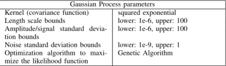
TABLE I: Parameters used when building the Kriging model, lb and ub denote the lower and upper bounds, respectively TABLE II: Number of variables (n) for WFG and DTLZ suites

WFG DTLZ k d l n n 2 4 4 8 6 3 4 4 8 7 5 8 4 12 9 10 18 4 22 14 g= mind(x0, x) (17) where x0 are the solutions belong the first front (or rank one solutions) and d(x0, x) = Pk_i₌₁fi(x0)−fi(x). For

instance, if a solution a dominates another solution b, then g(a, x0) > g(b, x0). Similar to DomRank, this function is not suitable for problems with many-objectives.

IV. NUMERICALEXPERIMENTS

This section provides a comparison of different functions after building surrogates on them. As mentioned we used the framework of EGO [22] and built Gaussian process mod-els as surrogates on the scalarizing functions. The expected improvement criterion in EGO is maximized with a genetic algorithm for selecting samples when updating the surrogates. The parameters of the Gaussian Process including kernel and bounds of hyperparameters are mentioned in Table I.

A. Performance of different scalarizing functions

To compare the performance of different scalarizing func-tions, we used DTLZ [49] and WFG [50] problems with 2, 3, 5 and 10 number of objectives. In DTLZ suite, the number of variables was kept to k+5-1, where k is the number of objectives. For the WFG suite, the number of variables is defined by position (d) and distance (l) parameters. For two objectives, d was set to four and 2×(k−1) for the rest of the objectives. The distance parameter was set to four for all objectives. To be summarized, the number of variables (n) for DTLZ and WFG suites is given in Table II:

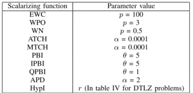
There are several parameters in different scalarizing func-tions and we used the recommended values from the respective articles. Different parameter values used are provided in Table

III. For WFG problems, the reference point r in HyPI is

used as 2×znadir. The vectorznadir contains the maximum objective function values in the Pareto front of the given prob-lem. We ran 21 independent runs for each scalarizing function with 300 maximum number of expensive function evaluations. We show the performance of different functions with inverted generational distance (IGD) and hypervolume. To compare the

(5)

TABLE III: Parameters values used in different scalarizing functions

Scalarizing function Parameter value

EWC p= 100 WPO p= 3 WN p= 0.5 ATCH α= 0.0001 MTCH α= 0.0001 PBI θ= 5 IPBI θ= 5 QPBI θ= 1 APD α= 2

HypI r(In table IV for DTLZ problems)

TABLE IV: Reference point in calculating hypevolumes in HypI and as performance measure

Problem reference point DTLZ1 400×(1,k) DTLZ2 1.5×(1,k) DTLZ3 900×(1,k) DTLZ4 2×(1,k) DTLZ5 1.5×(1,k) DTLZ6 6×(1,k) DTLZ7 5×(1,k)

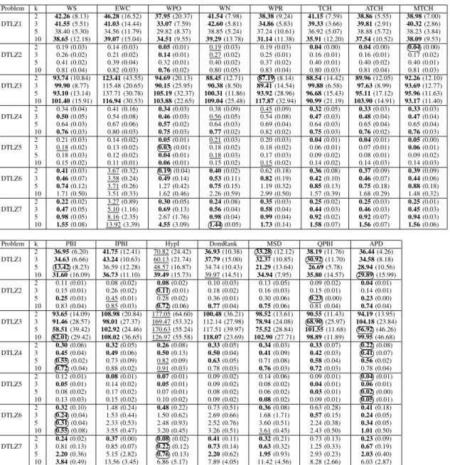
results of different functions, we used the Wilcoxon rank sum test with Bonferroni correction. The mean IGD values with standard deviation (in parentheses) for DTLZ problems are provided in Table V. The results with hypervolume and other detailed plots are in the supplementary material.

In Table V, the values statistically similar to the best value are in bold, the best value is in the circle and the worst value is underlined. As can be seen, the performance of different functions varies with different problems and three functions PBI, HypI, and APD outperformed other functions. Moreover, WS, ATCH, and DomRank never had the best IGD value in any of 64 instances. Note that, all these three functions have statistically similar values to the best IGD value in many cases. Another interesting observation from the results is that three different scalarizing functions ATCH, DomRank and MSD used in the literature for building surrogates on them were not in the top list. On the other hand, scalarizing functions used as the selection criterion in EMO algorithms e.g. APD and PBI performed significantly better. These results indicate that one needs to be cautious in selecting a scalarizing function in solving an expensive MOP.

B. Sensitivity towards number of objectives

When using scalarizing functions for building surrogates on them, the number of objectives can play a crucial role in their performance. Before using the surrogate built on the scalarizing function, we can analyze and visualize the fitness landscape with respect to uncertainty of predictions.

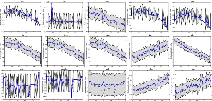
An example of fitness landscapes of DTLZ2 with two and 10 objectives for different scalarizing functions are shown in Figures 2 and 3, respectively. We used the same training data for all scalarizing functions. Then we generated a testing data set and used the model to get the predicted values (solid lines in figures) and uncertainties of the predicted values (shaded

region in figures). For visualization purposes, we could show only one of the variables values.

As can be seen, for the same training data set (and therefore same objective function values), different scalarizing functions gave different values. Therefore, the surrogate model to be built strongly depends on the g function values. For instance, in many-objective case, most of the solutions were nondominated and functions which used the property of Pareto dominance produced similar g values, as can be seen in the plots of DomRank, and MSD in 10 objective cases. As the g function values were the same for most of the solutions, the algorithm (EGO in this work) for finding a sample to update the surrogate by optimizing an infill criterion (EI in this work) was not able to enhance the accuracy of the surrogates. Scalarizing functions like APD and PBI did not use the property of Pareto dominance and suitable for a large number of objectives. In addition to the sensitivity towards many objectives, some functions, EWC and WS did not perform well in most of the problems. In EWC, the g function landscape is very rugged as can be seen in figures and WS has the problem of finding solutions in the non-convex parts of the Pareto front. These results show that one needs to see or analyze the landscape of scalarizing functions for the given training data set before using them in the optimization. We observed the similar behavior on other problems and landscapes on other problems with different objectives are provided in the supplementary material1_.

V. CONCLUSIONS

This work focused on reviewing, analyzing and compar-ing different scalarizcompar-ing functions in Bayesian multiobjective optimization for solving (computationally) expensive multi-and many-objective optimization problems. We provided an overview of different functions with their merits and demerits. We built the surrogates on the different functions and com-pared them with the different number of objectives. The results clearly showed that some functions outperformed others in many cases and some did not work in most of the cases. We then analyzed the fitness landscape of different functions with respect to the number of objectives. We found out that some functions are sensitive to the number of objectives. In this work, we did not compare the scalarizing functions with other methods which do not use scalarizing function. Therefore, comparison with other algorithms is a topic for future research.

ACKNOWLEDGEMENT

This research was supported by the Natural Environment Research Council, UK [grant number NE/P017436/1].

REFERENCES

[1] T. Chugh, K. Sindhya, J. Hakanen, and K. Miettinen, “A survey on han-dling computationally expensive multiobjective optimization problems with evolutionary algorithms,”Soft Computing, vol. 23, pp. 3137–3166, 2019.

(6)

0 0.2 0.4 0.6 0.8 1 x -0.2 0 0.2 0.4 0.6 0.8 1 1.2 1.4

Scalarizing function value

WS 0 0.2 0.4 0.6 0.8 1 x -4 -2 0 2 4 6 8

1084 EWC 0 0.2 0.4 0.6 0.8 1 x -0.2 0 0.2 0.4 0.6 0.8 1 1.2

WPO 0 0.2 0.4 0.6 0.8 1 x -0.2 0 0.2 0.4 0.6 0.8 1 1.2 1.4 1.6

WN 0 0.2 0.4 0.6 0.8 1 x -0.2 0 0.2 0.4 0.6 0.8 1 1.2

WPR 0 0.2 0.4 0.6 0.8 1 x -0.2 0 0.2 0.4 0.6 0.8 1 1.2

TCH 0 0.2 0.4 0.6 0.8 1 x -0.2 0 0.2 0.4 0.6 0.8 1 1.2

ATCH 0 0.2 0.4 0.6 0.8 1 x -0.2 0 0.2 0.4 0.6 0.8 1 1.2

MTCH 0 0.2 0.4 0.6 0.8 1 x -1 0 1 2 3 4 5 6 7

PBI 0 0.2 0.4 0.6 0.8 1 x -2 -1 0 1 2 3 4 5 6 7

IPBI 0 0.2 0.4 0.6 0.8 1 x -0.1 0 0.1 0.2 0.3 0.4 0.5 0.6 0.7 0.8 0.9

HypI 0 0.2 0.4 0.6 0.8 1 x 0.6 0.65 0.7 0.75 0.8 0.85 0.9 0.95 1 1.05 1.1

DomRank 0 0.2 0.4 0.6 0.8 1 x -1.2 -1 -0.8 -0.6 -0.4 -0.2 0 0.2

MSD 0 0.2 0.4 0.6 0.8 1 x -4000 -2000 0 2000 4000 6000 8000

QPBI 0 0.2 0.4 0.6 0.8 1 x 0.6 0.8 1 1.2 1.4 1.6 1.8 2

APD

Fig. 2: Approximated scalarizing function values (in solid line) with their uncertainty (in gray) on DTLZ2 two objectives. The dots represent the training data set.

0 0.2 0.4 0.6 0.8 1 x -0.2 0 0.2 0.4 0.6 0.8 1 1.2 1.4

WS 0 0.2 0.4 0.6 0.8 1 x -2 -1 0 1 2 3 4

1072 EWC 0 0.2 0.4 0.6 0.8 1 x -0.4 -0.2 0 0.2 0.4 0.6 0.8

WPO 0 0.2 0.4 0.6 0.8 1 x -1 -0.5 0 0.5 1 1.5 2 2.5 3

WN 0 0.2 0.4 0.6 0.8 1 x -0.04 -0.02 0 0.02 0.04 0.06 0.08 0.1 0.12

WPR 0 0.2 0.4 0.6 0.8 1 x -0.2 0 0.2 0.4 0.6 0.8 1

TCH 0 0.2 0.4 0.6 0.8 1 x -0.2 0 0.2 0.4 0.6 0.8 1

ATCH 0 0.2 0.4 0.6 0.8 1 x -0.2 0 0.2 0.4 0.6 0.8 1

MTCH 0 0.2 0.4 0.6 0.8 1 x 2 3 4 5 6 7 8 9 10 11

PBI 0 0.2 0.4 0.6 0.8 1 x 3 4 5 6 7 8 9 10 11

IPBI 0 0.2 0.4 0.6 0.8 1 x -2 0 2 4 6 8 10 12 14 16

HypI 0 0.2 0.4 0.6 0.8 1 x 0.94 0.95 0.96 0.97 0.98 0.99 1 1.01 1.02 1.03

DomRank 0 0.2 0.4 0.6 0.8 1 x -5 -4 -3 -2 -1 0 1 2

MSD 0 0.2 0.4 0.6 0.8 1 x -400 -200 0 200 400 600 800 1000 1200 1400

QPBI 0 0.2 0.4 0.6 0.8 1 x 0.4 0.6 0.8 1 1.2 1.4 1.6 1.8 2 2.2 2.4

APD

Fig. 3: Approximated scalarizing function values (in solid line) with their uncertainty (in gray) on DTLZ2 10 objectives. The dots represent the training data set.

(7)

Problem k WS EWC WPO WN WPR TCH ATCH MTCH 2 42.26(8.13) 46.28(16.52) 37.95(20.37) 41.54(7.98) 38.38(9.24) 41.15(7.59) 38.86(5.55) 38.98(7.00) DTLZ1 3 41.55(5.51) 41.03(14.44) 33.07(7.59) 42.60(5.81) 34.86(5.83) 39.33(3.66) 39.81(2.91) 40.32(2.86) 5 38.40 (5.30) 34.56 (11.79) 29.82 (8.37) 38.85 (5.24) 37.24 (10.61) 36.92 (5.07) 38.88 (5.72) 38.23 (3.84) 10 38.65(12.18) 39.07(15.04) 34.51(9.55) 39.29(13.78) 31.14(11.38) 35.91(12.20) 37.54(10.52) 38.09(9.53) 2 0.19 (0.03) 0.14 (0.03) 0.05(0.01) 0.19 (0.03) 0.19 (0.03) 0.04(0.00) 0.04(0.00) 0.04(0.00) DTLZ2 3 0.26 (0.02) 0.21 (0.02) 0.14(0.01) 0.27 (0.02) 0.25 (0.01) 0.16 (0.01) 0.16 (0.01) 0.17 (0.02) 5 0.41 (0.02) 0.39 (0.04) 0.32 (0.01) 0.40 (0.02) 0.37 (0.02) 0.40 (0.01) 0.40 (0.02) 0.40 (0.01) 10 0.81 (0.04) 0.82 (0.03) 0.76(0.02) 0.80 (0.05) 0.83 (0.04) 0.80 (0.03) 0.81 (0.04) 0.81 (0.03) 2 93.74(10.84) 123.41(43.55) 94.69(20.13) 88.45(12.71) 87.19(8.14) 88.54(14.42) 89.96(12.05) 92.26(12.10) DTLZ3 3 99.90(8.77) 115.48 (20.65) 90.15(25.95) 90.38(8.50) 89.41(14.54) 99.88(6.58) 97.63(8.99) 93.69(12.77) 5 93.10(13.14) 137.71 (30.78) 105.19(32.37) 100.31(11.86) 93.92(28.96) 96.68(15.43) 95.11(17.12) 95.96(11.63) 10 101.40(15.91) 116.94(30.53) 103.88(22.65) 109.04(25.48) 117.87(32.94) 90.99(21.19) 103.90(14.91) 93.17(11.40) 2 0.34 (0.04) 0.41 (0.16) 0.34(0.03) 0.38 (0.09) 0.45 (0.09) 0.32(0.05) 0.33(0.03) 0.33(0.03) DTLZ4 3 0.50(0.05) 0.54 (0.08) 0.46(0.03) 0.56 (0.05) 0.54 (0.08) 0.47(0.03) 0.48(0.04) 0.47(0.04) 5 0.64 (0.03) 0.67 (0.06) 0.57(0.02) 0.64 (0.03) 0.69 (0.04) 0.64 (0.03) 0.65 (0.04) 0.65 (0.04) 10 0.76(0.03) 0.80 (0.03) 0.75(0.03) 0.77(0.02) 0.82 (0.02) 0.75(0.03) 0.76(0.02) 0.76(0.03) 2 0.21 (0.03) 0.14 (0.02) 0.05(0.01) 0.21 (0.03) 0.20 (0.03) 0.04(0.01) 0.04(0.01) 0.05(0.00) DTLZ5 3 0.18 (0.02) 0.13 (0.02) 0.03(0.01) 0.18 (0.02) 0.18 (0.02) 0.06 (0.01) 0.07 (0.01) 0.06(0.01) 5 0.18 (0.03) 0.12 (0.02) 0.04(0.01) 0.18 (0.03) 0.17 (0.03) 0.09 (0.02) 0.08 (0.01) 0.09 (0.02) 10 0.15 (0.02) 0.11 (0.01) 0.06(0.01) 0.15 (0.02) 0.15 (0.02) 0.14 (0.02) 0.14 (0.03) 0.14 (0.03) 2 0.41(0.03) 3.67 (0.32) 0.19(0.04) 0.40(0.02) 0.62 (0.18) 0.36(0.08) 0.37(0.09) 0.39(0.09) DTLZ6 3 0.46(0.07) 3.58 (0.24) 0.49(0.14) 0.53(0.11) 0.82(0.19) 0.42(0.10) 0.46(0.07) 0.44(0.06) 5 0.74(0.12) 3.71 (0.26) 1.27 (0.42) 0.75(0.15) 1.19 (0.32) 0.85(0.13) 0.75(0.18) 0.88(0.18) 10 1.71 (0.50) 3.51 (0.33) 1.62 (0.46) 2.26 (0.59) 2.99 (0.50) 1.57 (0.39) 1.68 (0.29) 1.48 (0.32) 2 0.22(0.02) 3.27 (0.89) 0.30(0.05) 0.24(0.08) 0.35(0.03) 0.25(0.02) 0.25(0.03) 0.25(0.01) DTLZ7 3 0.47(0.05) 5.10 (1.16) 0.69(0.13) 0.56(0.04) 0.58(0.04) 0.44(0.03) 0.46(0.03) 0.45(0.03) 5 0.98(0.05) 8.16 (2.35) 2.67 (1.76) 0.98(0.04) 0.99(0.04) 0.92(0.02) 0.92(0.07) 0.94(0.03) 10 1.55(0.08) 13.92 (3.39) 4.55(3.09) 1.44(0.05) 1.73(0.14) 1.58(0.07) 1.56(0.07) 1.56(0.06)

Problem k PBI IPBI HypI DomRank MSD QPBI APD

2 36.95(6.20) 41.75(12.41) 70.82 (24.42) 36.93(10.38) 33.28(12.12) 38.19(11.76) 36.44(4.26) DTLZ1 3 34.63(6.66) 43.24(10.63) 60.13 (21.74) 37.79(15.00) 32.37(10.85) 30.92(11.70) 34.58(8.18) 5 13.42(8.23) 36.59 (12.28) 48.57 (16.87) 34.74 (10.43) 21.29(13.64) 26.69(5.78) 28.94(10.56) 10 31.60(16.09) 36.73(11.10) 39.49(15.73) 39.97 (14.51) 34.94(7.95) 35.80(14.57) 29.89(15.99) 2 0.11 (0.01) 0.08 (0.02) 0.08(0.02) 0.10 (0.03) 0.13 (0.05) 0.09 (0.02) 0.04(0.01) DTLZ2 3 0.15 (0.01) 0.26 (0.02) 0.11(0.01) 0.18 (0.02) 0.16 (0.03) 0.15 (0.01) 0.14 (0.01) 5 0.25(0.01) 0.45 (0.01) 0.28 (0.02) 0.36 (0.01) 0.30 (0.06) 0.23(0.00) 0.23(0.00) 10 0.83 (0.04) 0.85 (0.03) 0.72(0.06) 0.77(0.04) 0.75(0.06) 0.81 (0.04) 0.74(0.04) 2 93.65(14.09) 108.98(20.84) 177.05 (64.60) 100.48(36.21) 98.52(13.61) 90.55(11.43) 94.19(13.95) DTLZ3 3 91.46(28.57) 98.01(27.37) 169.47 (53.32) 112.14 (27.98) 78.94(24.08) 68.90(25.97) 104.18(23.84) 5 58.51(39.42) 102.92(24.46) 170.63 (55.24) 117.51 (39.97) 75.52(28.84) 101.55(11.68) 56.92(46.26) 10 82.01(29.42) 108.02(36.65) 126.97 (55.58) 118.07(23.69) 102.90(27.71) 98.89(11.89) 99.95(46.68) 2 0.30(0.06) 0.32(0.05) 0.26(0.08) 0.33(0.05) 0.34(0.03) 0.33(0.07) 0.22(0.08) DTLZ4 3 0.45(0.04) 0.49(0.06) 0.50(0.13) 0.50(0.04) 0.41(0.09) 0.42(0.03) 0.41(0.07) 5 0.55(0.02) 0.73 (0.09) 0.82 (0.09) 0.63(0.05) 0.71 (0.08) 0.58(0.04) 0.56(0.02) 10 0.72(0.04) 0.88 (0.02) 0.91 (0.03) 0.78 (0.03) 0.76(0.03) 0.72(0.03) 0.78 (0.04) 2 0.12 (0.01) 0.08(0.01) 0.07(0.01) 0.09 (0.02) 0.14 (0.06) 0.09 (0.01) 0.04(0.01) DTLZ5 3 0.05(0.01) 0.14 (0.02) 0.05(0.01) 0.09 (0.02) 0.08 (0.02) 0.04(0.01) 0.06(0.01) 5 0.08 (0.02) 0.17 (0.02) 0.07 (0.01) 0.08 (0.02) 0.06 (0.02) 0.03(0.01) 0.02(0.00) 10 0.13 (0.03) 0.15 (0.02) 0.10 (0.02) 0.09 (0.02) 0.08(0.02) 0.09 (0.01) 0.05(0.01) 2 0.32(0.10) 1.48 (0.24) 0.48(0.22) 0.73 (0.51) 0.36(0.08) 0.63 (0.28) 0.41(0.18) DTLZ6 3 0.24(0.04) 1.53 (0.44) 1.50 (0.62) 2.69 (0.66) 1.68 (1.71) 0.57(0.15) 0.24(0.05) 5 0.31(0.04) 2.33 (0.53) 2.48 (0.93) 2.52 (0.76) 3.60 (0.51) 2.24 (0.38) 0.34(0.05) 10 0.55(0.08) 3.55 (0.47) 3.20 (0.45) 3.26 (0.51) 3.61 (0.45) 2.43 (0.50) 1.01(0.50) 2 0.24(0.02) 0.37(0.00) 0.08(0.02) 0.41(0.11) 0.32(0.21) 0.73 (0.13) 0.23(0.09) DTLZ7 3 0.81 (0.13) 0.85 (0.07) 0.22(0.12) 0.73(0.14) 0.63(0.32) 1.25 (0.33) 0.67(0.19) 5 2.20(0.36) 5.15 (2.82) 0.76(0.13) 2.20(0.62) 1.95(0.93) 2.93 (0.23) 2.03(0.40) 10 3.84(0.49) 13.56 (3.45) 6.86 (5.17) 7.89 (4.05) 11.42 (4.56) 8.28 (2.66) 6.03 (2.87)

TABLE V: Mean IGD values and standard deviation (in parentheses) for DTLZ problems. The values statistically similar to the best one are in bold, the best value is encircled the worst value is underlined

[2] Y. Jin, “Surrogate-assisted evolutionary computation: Recent advances and future challenges,”Swarm and Evolutionary Computation, vol. 1, pp. 61–70, 2011.

[3] R. Allmendinger, M. Emmerich, J. Hakanen, Y. Jin, and E. Rigoni, “Surrogate-assisted multicriteria optimization: Business case, complexi-ties and prospective solutions,”Multi-Criteria Decision Analysis, vol. 24, pp. 5–24, 2017.

[4] K. Deb, R. Hussein, P. C. Roy, and G. Toscano, “A taxonomy for meta-modeling frameworks for evolutionary multi-objective optimization,”

IEEE Transactions on Evolutionary Computation, vol. 23, pp. 104–116,

2019.

[5] D. Horn, T. Wagner, D. Biermann, C. Weihs, and B. Bischl, “Model-based multi-objective optimization: Taxonomy, multi-point proposal, toolbox and benchmark,” inEvolutionary Multi-criterion Optimization, A. Gasper-Cunha, C. H. Antunes, and C. Coello, Eds. Springer, 2015, pp. 64–78.

[6] M. Mckay, R. Beckman, and W. Conover, “A comparison of three methods for selecting values of input variables in the analysis of output from a computer code,”Technometrics, vol. 42, pp. 55–61, 2000. [7] T. Chugh, A. Rahat, V. Volz, and M. Zaefferer, High-Performance

Simulation Based Optimization. Springer, 2020, vol. 833, ch. Towards

Better Integration of Surrogate Models and Optimizers, pp. 137–163. [8] T. Chugh, Y. Jin, K. Miettinen, J. Hakanen, and K. Sindhya, “A

surrogate-assisted reference vector guided evolutionary algorithm for computationally expensive many-objective optimization,”IEEE

Trans-actions on Evolutionary Computation, vol. 22, pp. 129 – 142, 2018.

[9] W. Ponweiser, T. Wagner, D. Biermann, and M. Vincze, “Multiobjective optimization on a limited budget of evaluations using model-assisted S-metric selection,” inProceedings of the Parallel Problem Solving from

Nature-PPSN X. Springer, 2008, pp. 784–794.

[10] Q. Zhang, W. Liu, E. Tsang, and B. Virginas, “Expensive multiobjective optimization by MOEA/D with gaussian process model,”IEEE

Trans-actions on Evolutionary Computation, vol. 14, pp. 456–474, 2010.

[11] J. Knowles, “ParEGO: a hybrid algorithm with on-line landscape ap-proximation for expensive multiobjective optimization problems,”IEEE

Transactions on Evolutionary Computation, vol. 10, pp. 50–66, 2006.

[12] A. A. M. Rahat, R. M. Everson, and J. E. Fieldsend, “Alternative infill strategies for expensive multi-objective optimisation,” inProceedings of

the Genetic and Evolutionary Computation Conference. ACM, 2017,

(8)

[13] L. Pan, C. He, Y. Tian, H. Wang, X. Zhang, and Y. Jin, “A classification based surrogate-assisted evolutionary algorithm for expensive many-objective optimization,”IEEE Transactions on Evolutionary Computa-tion, vol. 23, pp. 74–88, 2019.

[14] I. Loshchilov, M. Schoenauer, and M. Sebag, “Dominance-based Pareto-surrogate for multi-objective optimization,” inProceedings of the

Simu-lated Evolution and Learning, K. Deb, A. Bhattacharya, N. Chakroborty,

S. Das, J. Dutta, S. Gupta, A. Jain, V. Aggarwal, J. Branke, S. Louis, and K. Tan, Eds. Springer, 2010, pp. 230–239.

[15] S. Bandaru, A. Ng, and K. Deb, “On the performance of classification algorithms for learning Pareto-dominance relations,” inProceedings of

the IEEE Congress on Evolutionary Computation. IEEE, 2014, pp.

1139–1146.

[16] T.Chugh, A. Rahat, and P. Palar, “Trading-off data fit and complexity in training gaussian processes with multiple kernels,” inProceedings of the International Conference on Machine Learning, Optimization, and

Data Science (LOD), ser. Lecture Notes in Computer Science (LNCS).

Springer, 2019, pp. 579–591.

[17] M. Pescador-Rojas, R. Hern´andez G´omez, E. Montero, N. Rojas-Morales, M.-C. Riff, and C. A. Coello Coello, “An overview of weighted and unconstrained scalarizing functions,” in Evolutionary

Multi-Criterion Optimization, H. Trautmann, G. Rudolph, K. Klamroth,

O. Sch¨utze, M. Wiecek, Y. Jin, and C. Grimme, Eds. Springer, 2017, pp. 499–513.

[18] H. Ishibuchi, Y. Setoguchi, H. Masuda, and Y. Nojima, “Performance of decomposition-based many-objective algorithms strongly depends on pareto front shapes,”IEEE Transactions on Evolutionary Computation, vol. 21, no. 2, pp. 169–190, 2017.

[19] R. G´omez and C. Coello, “A hyper-heuristic of scalarizing functions,” in

Proceedings of the Genetic and Evolutionary Computation Conference.

ACM, 2017, pp. 577–584.

[20] K. Miettinen and M. M. M¨akel¨a, “On scalarizing functions in multiob-jective optimization,”OR Spectrum, vol. 24, pp. 193–213, 2002. [21] K. Miettinen, Nonlinear multiobjective optimization. Boston, MA:

Kluwer, 1999.

[22] D. Jones, M. Schonlau, and W. Welch, “Efficient global optimization of expensive black-box functions,”Journal of Global Optimization, vol. 13, pp. 455–492, 1998.

[23] C.-L. Hwang and A. Masud, Multiple Objective Decision

Making-Methods and Applications. Springer, 1979.

[24] R. E. Steuer,Multiple Criteria Optimization: Theory, Computation and

Application. New York: John Wiley & Sons, 1986.

[25] K. Deb and H. Jain, “An evolutionary many-objective optimization algorithm using reference-point-based nondominated sorting approach, part I: solving problems with box constraints,”IEEE Transactions on

Evolutionary Computation, vol. 18, pp. 577–601, 2014.

[26] Q. Zhang and H. Li, “MOEA/D: A multiobjective evolutionary algorithm based on decomposition,”IEEE Transactions on Evolutionary

Compu-tation, vol. 11, pp. 712–731, 2007.

[27] A. Trivedi, D. Srinivasan, K. Sanyal, and A. Ghosh, “A survey of multiobjective evolutionary algorithms based on decomposition,”IEEE

Transactions on Evolutionary Computation, vol. 21, pp. 440–462, June

2017.

[28] R. Cheng, Y. Jin, M. Olhofer, and B. Sendhoff, “A reference vector guided evolutionary algorithm for many-objective optimization,” IEEE

[29] H. Ishibuchi, N. Tsukamoto, and Y. Nojima, “Evolutionary many-objective optimization: A short review,” in Proceedings of IEEE

Congress on Evolutionary Computation. IEEE, 2008, pp. 2419–2426.

[30] B. Li, J. Li, K. Tang, and X. Yao, “Many-objective evolutionary algorithms: A survey,” ACM Computing Surveys, vol. 48, pp. 13–35, 2015.

[31] H. Ishibuchi, Y. Sakane, N. Tsukamoto, and Y. Nojima, “Simultaneous use of different scalarizing functions in MOEA/D,” inProceedings of

the 12th Annual Conference on Genetic and Evolutionary Computation.

ACM, 2010, pp. 519–526.

[32] H. Ishibuchi, K. Doi, and Y. Nojima, “Use of piecewise linear and non-linear scalarizing functions in MOEA/D,” inParallel Problem Solving

from Nature – PPSN XIV, J. Handl, E. Hart, P. R. Lewis, M.

López-Ibáñez, G. Ochoa, and B. Paechter, Eds. Springer, 2016, pp. 503–513. [33] B. Derbel, D. Brockhoff, A. Liefooghe, and S. Verel, “On the impact of multiobjective scalarizing functions,” in Parallel Problem Solving

from Nature – PPSN XIII, T. Bartz-Beielstein, J. Branke, B. Filipiˇc,

and J. Smith, Eds. Springer, 2014, pp. 548–558.

[34] R. Hern´andez G´omez and C. A. Coello Coello, “Improved metaheuristic based on the r2 indicator for many-objective optimization,” in Pro-ceedings of the 2015 Annual Conference on Genetic and Evolutionary

Computation. ACM, 2015, pp. 679–686.

[35] M. C. Riff and E. Montero, “A new algorithm for reducing metaheuristic design effort,” in2013 IEEE Congress on Evolutionary Computation, 2013, pp. 3283–3290.

[36] M. T. M. Emmerich and A. H. Deutz, “Test problems based on lam´e superspheres,” inProceedings of the 4th International Conference

on Evolutionary Multi-criterion Optimization, ser. EMO’07. Berlin,

Heidelberg: Springer-Verlag, 2007, pp. 922–936.

[37] D. Hardin and E. B. SAFF, “Discretizing manifolds via minimum energy points,”Notices of the American Mathematical Society, vol. 51, 2004. [38] S. Jiang, S. Yang, Y. Wang, and X. Liu, “Scalarizing functions

in decomposition-based multiobjective evolutionary algorithms,”IEEE

[39] H. Li, Q. Zhang, and J. Deng, “Biased multiobjective optimization and decomposition algorithm,”IEEE Transactions on Cybernetics, vol. 47, no. 1, pp. 52–66, 2017.

[40] C. E. Rasmussen and C. K. I. Williams,Gaussian processes for machine

learning. The MIT Press, 2006.

[41] J. Cornell,Experiments with Mixtures: Designs, Models, and the

Anal-ysis of Mixture Data. John Wiley & Sons, 2011.

[42] K. Deb, A. Prarap, S. Agarwal, and T. Meyarivan, “A fast and elitist multiobjective genetic algorithm: NSGA-II,” IEEE Transactions on

Evolutionary Computation, vol. 6, pp. 182–197, 2002.

[43] C. Coello, G. Lamont, and D. Veldhuizen,Evolutionary Algorithms for

Solving Multi-objective Problems, 2nd ed. New York: Springer, New

York, 2007.

[44] T. Athan and P. Papalambros, “A note on the weighted criteria methods for compromise solutions in multi-objective optimization,”Engineering

Optimization, vol. 27, no. 2, pp. 155–176, 1996.

[45] I. Kaliszewski, “A modified weighted tchebycheff metric for multiple objective programming,” Computers Operations Research, vol. 14, no. 4, pp. 315 – 323, 1987.

[46] H. Ishibuchi, Y. Hitotsuyanagi, Y. Wakamatsu, and Y. Nojima, “How to choose solutions for local search in multiobjective combinatorial memetic algorithms,” in Proceedings of the Parallel Problem

Solv-ing from Nature-PPSN XI, R. Schaefer, C. Cotta, J. Kolodziej, and

G. Rudolph, Eds. Springer, 2010, pp. 516–525.

[47] H. Sato, “Inverted PBI in MOEA/D and its impact on the search per-formance on multi and many-objective optimization,” inProceedings of

the 2014 Annual Conference on Genetic and Evolutionary Computation.

ACM, 2014, pp. 645–652.

[48] C. Fonseca and P. Fleming, “Genetic algorithms for multiobjective op-timization: Formulation, discussion and generalization,” inProceedings

of the Fifth International Conference on Genetic Algorithms, S. Forrest,

Ed. Morgan Kaufmann, 1993, pp. 416–423.

[49] K. Deb and H. Gupta, “Searching for robust Pareto-optimal solutions in multi-objective optimization,” in Proceedings of the Evolutionary

Multi-Criterion Optimization, C. Coello, A. Aguirre, and E. Zitzler, Eds.

Springer, 2005, pp. 150–164.

[50] S. Huband, L. Barone, L. While, and P. Hingston, “A scalable multi-objective test problem toolkit,” in Evolutionary Multi-Criterion

Opti-mization, C. Coello, A. H. Aguirre, and E. Zitzler, Eds. Springer,