Probabilistic and Deep Learning Algorithms for the Analysis of Imagery Data

(1)

Louisiana State University

LSU Digital Commons

LSU Doctoral Dissertations Graduate School

2016

Probabilistic and Deep Learning Algorithms for the

Analysis of Imagery Data

Saikat Basu

Louisiana State University and Agricultural and Mechanical College

Follow this and additional works at:https://digitalcommons.lsu.edu/gradschool_dissertations

Part of theComputer Sciences Commons

This Dissertation is brought to you for free and open access by the Graduate School at LSU Digital Commons. It has been accepted for inclusion in LSU Doctoral Dissertations by an authorized graduate school editor of LSU Digital Commons. For more information, please [email protected]. Recommended Citation

Basu, Saikat, "Probabilistic and Deep Learning Algorithms for the Analysis of Imagery Data" (2016).LSU Doctoral Dissertations. 2428.

(2)

PROBABILISTIC AND DEEP LEARNING ALGORITHMS FOR THE ANALYSIS OF IMAGERY DATA

A Dissertation

Submitted to the Graduate Faculty of the Louisiana State University and Agricultural and Mechanical College

in partial fulfillment of the requirements for the degree of

Doctor Of Philosophy in

The Department of Computer Science

by Saikat Basu

B.Tech, National Institute of Technology Durgapur, 2011 December 2016

(3)

(4)

Acknowledgments

This research was supported by NASA Carbon Monitoring System through Grant #NNH14Z DA001-N-CMS and Army Research Office (ARO) under Grant #W911NF1010495 and was par-tially supported by the Cooperative Agreement Number NASA-NNX12AD05A, CFDA Number 43.001, for the project identified as ”Ames Research Center Cooperative for Research in Earth Science and Technology (ARC-CREST)”. Any opinions findings, and conclusions or recommen-dations expressed in this material are those of the authors and do not necessarily reflect that of NASA, ARO or the United States Government. The research was also partially supported by the AWS Climate Research Grant. We are grateful to the United States Department of Agriculture for providing us the National Agriculture Imagery Program (NAIP) airborne imagery dataset for the Continental United States.

I would like to thank my advisor Supratik Mukhopadhyay for his constant help and guidance and for motivating me to pursue research in Deep Learning. I am also thankful to my commit-tee members Costas Busch, Jianhua Chen, Hartmut Kaiser and Ye-Sho Chen for providing me valuable feedback and in reviewing my research work. I am also thankful to the members of my research group Robert DiBiano, Manohar Karki and Malcolm Stagg for their time and support.

I would also like to thank Sangram Ganguly, Ramakrishna Nemani, Andrew Michaelis, Petr Votava, Uttam Kumar, Cristina Milesi and other members from NASA Ames Research Center who helped and guided me during various phases of my research.

I am thankful to Ananya for putting up with me and Subhajit, Sayan, Arnab, Sujana, Ishita, Trina, Arghya, Satadru and Joy for those amazing weekends and the delicious food. I am also thankful to Ayan for the inspiring conversations. Finally, I would like to thank Baba, Maa and Didi for being there with me at every turn of my life and for being a constant source of motivaton.

(5)

List of Tables

2.1 Distance between Means and Standard Deviations for raw image values and the Extracted feature vectors for a sample set of 5000 randomly selected labeled image patches from the NAIP dataset for

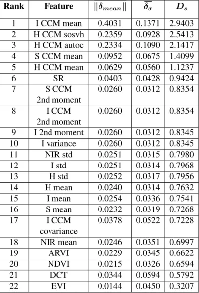
the state of California. . . 14 2.2 Ranking of features based on Distribution Separability Criterion for

the sample dataset. . . 15 2.3 Classification Accuracy of the classifier with various network

archi-tectures using the entire set of 150 features and the set of 22 features

derived using the feature selection method presented in Section 2.3.2 . . . 38 2.4 Preliminary classification accuracy assessment. . . 38 2.5 Confusion Matrix . . . 41 2.6 Comparative results with NLCD for fragmented forests (top) and

urban forested areas (bottom).[113] . . . 41 3.1 Classification Accuracy of DBN with various architectures on

SAT-4 and SAT-6 . . . 54 3.2 Classification Accuracy of CNN with various architectures on SAT-4 . . . 55 3.3 Classification Accuracy of SAE with various architectures on SAT-4

and SAT-6 . . . 57 3.4 Classification Accuracy of DeepSat with various network

architec-tures on SAT-4 and SAT-6 . . . 61 3.5 Training and Test times of a traditional DBN and DeepSat on SAT-4

and SAT-6 . . . 61 3.6 Distance between Means and Standard Deviations for raw image

values and DeepSat feature vectors for SAT-4 and SAT-6 . . . 62 3.7 Ranking of features based on Distribution Separability Criterion for

SAT-6 . . . 64 3.8 Intrinsic Dimension estimation using DANCo on the MNIST,

CIFAR-10, and SAT-6 datasets and the Haralick features extracted from the

SAT-6 dataset. . . 65 4.1 Test Error of a traditional DBN and our framework with various

(9)

4.2 Test Error of a traditional DBN and our framework with various architectures on n-MNIST with Motion Blur; and with AWGN and

Reduced Contrast . . . 77 4.3 Test Error of a traditional DBN and our framework with various

architectures on the noisy Bangla dataset with AWGN . . . 78 4.4 Test Error of a traditional DBN and our framework with various

architectures on noisy Bangla dataset with Motion Blur; and with

AWGN and Reduced Contrast . . . 78 4.5 Mean contrast of the MNIST and Bangla numeral datasets. . . 78 5.1 Intrinsic Dimension estimation using MLE on the MNIST,

CIFAR-10 and DET datasets . . . 90 5.2 Intrinsic Dimension estimation using MLE on the 6 texture datasets . . . 90 5.3 Mean distance from origin to closest data point for various object

recognition and texture datasets . . . 93 5.4 Test Error of a Convolutional Neural Network trained using

(10)

List of Figures

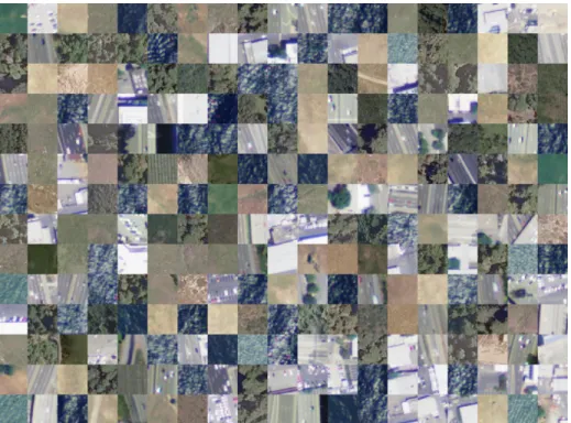
2.1 A sample of image patches from the NAIP dataset showing tree and

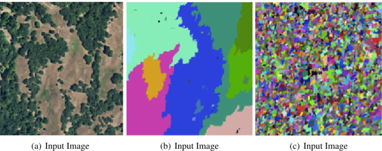
non-tree areas. . . 10 2.2 Example NAIP input image and under-segmented and over-segmented

outputs from the Statistical Region Merging Algorithm. Under-segmentation creates interclass overlaps within a segment while over-segmentation avoids inter-class overlaps within a segment by creat-ing mutually exclusive segments with pixels belongcreat-ing to only one

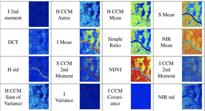
class. . . 12 2.3 Example Features extracted from a sample NAIP tile. . . 13 2.4 The neighborhood system for the pixelpLwhererL−pL=δ. . . 16

2.5 (a) A sample NAIP tile and the CRF output probability maps with (b) the unary term φp(xp), (c) the combination of the unary term

φp(xp)and the pairwise termφpq(xp, xq)and (d) the combination of

the unary termφp(xq), the pairwise termφpq(xp, xq)and the region

consistency termφc(xc). . . 22

2.6 Variation of Omission and Commision Errors with changing epochs

of the online update algorithm. . . 25 2.7 A sample NAIP tile with tree and non-tree cover masks generated by

the Random Walker Segmentation module by selecting a certain set of foreground and background seed pixels. The small red squares indicate the training samples extracted from the image which are in turn saved to the training database with the correct label. Note that only complete squares representing4×4training images are saved

to the database while the rest are discarded. . . 27 2.8 High Performance Computing Architecture of our approach. . . 28

(11)

2.9 ROC Curves for the three types of landscapes considered – frag-mented, urban and densely forested (The numbers indicate the cor-responding window sizes). One representative NAIP tile was cho-sen for each landscape – a densely forested tile from the Gasquet region in Northwestern California (7750m × 6380m), a tile with fragmented forests from the Susanville region in Northeastern Cal-ifornia (7610m ×6000m), and an urban tile from a region in San Jose, California (7620m×6240m). 5000 points were chosen ran-domly from each image tile, labels for these representative points were assigned by a human expert and the tree cover maps were val-idated against these ground truth data to generate the true positive

rate and false positive rate for the ROC Curves. . . 29 2.10 Performance of the Neural Network training algorithm for a set of

(randomly chosen) 3500 training samples, 750 validation samples and 750 test samples from a NAIP tile from Blocksburg, Califor-nia (7610m× 6000m). The X-axis marks the iterations/epochs of the training algorithm, while the mean-squared error is noted along the Y-axis. The blue line indicates the mean squared error at var-ious epochs during the training phase of the Neural Network, the green line indicates the mean squared validation error and the red line indicates the mean squared test error. The best performance is

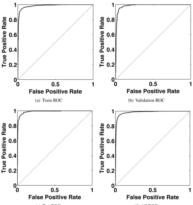
attained at iteration 72. . . 30 2.11 ROC Curves for the Neural Network Training algorithm for the

same dataset used in Figure 2.10 – ROC curve generated for train-ing, validation, test sets and taking the mean of the true positive rate and false positive rate of the training, validation and test dataset

re-spectively. . . 31 2.12 Confusion Matrix for the Neural Network training algorithm for the

dataset used in Figure 2.10 and Figure 2.11. A total of 3500 samples are used for training, 750 samples for validation and 750 samples

for testing. . . 32 2.13 Results for an image tile with fragmented trees in Hoopa,

Califor-nia, north of the Klamath River and an urban area in San Jose,

Cal-ifornia for NLCD and NAIP. . . 33 2.14 ROC Curve generated by changing the sample size of the training

data. The region of study was the same as that of Figure 2.10 – an area with fragmented forests in the Blocksburg region in northwest-ern California (7610 m×6000 m). The numbers denote the number

(12)

2.15 ROC Curve generated by changing the Quantization Level in the SRM algorithm for the same area as considered in Figure 2.14. The training sample size is 5000 - consisting of 2500 tree and 2500 non-tree samples chosen at random from the NAIP tile. The numbers

denote the corresponding Qlevel values. . . 35 2.16 Probability Maps for the probabilistic NN classifier results (a-c) and

CRF output (d-f) for various training sample sizes (1300,1800 and 2500 samples per class from left to right) for a sample NAIP tile from Blocksburg, California. The color maps show the probabili-ties on a scale of 0 to 1. The probability maps for the NN represent the probability of a pixel being predicted as a tree by the Neural Net-work and the probability maps for the CRF output represent the final probabilities assigned to the pixels by the CRF labeling algorithm. A pixel assuming a value of 1 in the probability map is marked as a tree and a pixel assuming a value of 0 is marked as a non-tree, with intermediate pixels values being marked as tree/non-tree according to the problem (here, we use a 50% threshold, i.e., a pixel is marked

as tree if the probability exceeds 0.5). . . 36 2.17 (a) A sample image with (b) the final Probability Map generated

by our framework for a region in Blocksburg, California. This fi-nal probability map is the same as the map generated by the CRF based labeling algorithm as shown in Figure 2.16. The CRF al-gorithm combines the probability values assumed by the classifier outputs for individual pixels and generates the final probability map

as shown above. . . 37 2.18 The validation error rate for the same dataset used in Figure 2.10

for the 100-100 and 100-100-100 neural networks without ization, and the 100-100-100 neural network with L2 norm

regular-ization and Dropout. . . 39 2.19 A satellite image showing the validation points chosen for our

ex-periments over California. The red circles denote the validation points. A total of 36000 sampling points were chosen to repre-sent densely forested areas, fragmented forests and urban forested areas of California. The green grid represents the individual NAIP tiles. In order to display the locations from which the validation points were sampled, multiple points were clustered into subgroups and hence each red circle in the figure represents multiple validation

(13)

2.20 The final tree-cover maps generated using LiDAR (left) and NAIP (right) for Area 1 (top) and Area 2 (bottom). The green regions rep-resent tree cover areas, the white regions reprep-resent non-tree areas and the black regions represent the areas with null values in the Li-DAR data (these black regions were masked out from the NAIP tree

cover maps for comparative studies with the corresponding LiDAR maps). . . 42 2.21 Percentage of forest cover obtained using Neural Network and

Ran-dom Forest (for NAIP), and NLCD and LiDAR in Area 1 (the west-ern Sierra Nevada mountain range over the Teakettle Experimental Forest in California). A 50×50 sliding window was used to obtain the percentage of tree-cover pixels in both NAIP and NLCD with

LiDAR as the ground truth. . . 43 2.22 Percentage of non-forest area obtained using Neural Network and

Random Forest (for NAIP), and NLCD and LiDAR in Area 1 (same

as the area in Figure 2.21). The sliding window size was 50×50. . . 43 2.23 True Positive Rate (TPR) and False Positive Rate (FPR) of Neural

Network and Random Forest (for NAIP) and NLCD with LiDAR as ground truth for Area 1 (same as the area in Figure 2.21). The

sliding window size was 50×50. . . 44 2.24 Percentage of forest cover obtained using Neural Network and

Ran-dom Forest (for NAIP), and NLCD and LiDAR for Area 2 (the Chester area in California). The sliding window size was kept as

50×50. . . 44 2.25 Percentage of non-forest area obtained using Neural Network and

Random Forest (for NAIP), and NLCD and LiDAR for Area 2 (same

as Figure 2.24) with the sliding window size kept constant at 50×50. . . 45 2.26 True Positive Rate (TPR) and False Positive Rate (FPR) of the

Neu-ral Network and Random Forest (for NAIP) and NLCD with LiDAR as ground truth for Area 2 (same as the area in Figure 2.21). The

sliding window size was 50×50. . . 45 2.27 A sample NAIP tile (left) and the corresponding binary tree cover

mask (right). The white pixels denote non-tree areas while the green

pixels denote the tree-cover areas. . . 46 2.28 The final tree cover map generated by our framework for the whole

of California covering 11,095 NAIP tiles. The green pixels denote

the tree-cover areas while the white pixels denote the non-tree areas. . . 47 3.1 Sample images from the SAT-6 dataset . . . 51

(14)

3.2 Schematic of the classification framework . . . 57 3.3 Distributions of the raw NIR values for traditional Deep Learning

Algorithms and a sample DeepSat feature for various classes on

SAT-4 (Best viewed in color) . . . 62 3.4 Distribution Separability Criterion of the neurons in the layers of a

DBN and DeepSat with various architectures on SAT-6 . . . 65 4.1 Example images from the n-MNIST dataset created as part of the experiments.. . . 70 4.2 Example images from the noisy Bangla dataset created as part of the experiments. . 71 5.1 Test Error on the 6 texture datasets with the Haralick features and

stacked Restricted Boltzmann Machines with L2 norm regulariza-tion, Dropout and Dropconnect obtained by varying the number of

adjustable parameters. . . 97 5.2 Test Error on the 6 texture datasets with the Haralick features and

Stacked Denoising Autoencoders withL2norm regularization, Dropout and Dropconnect obtained by varying the number of adjustable

(15)

Abstract

Accurate object classification is a challenging problem for various low to high resolution imagery data. This applies to both natural as well as synthetic image datasets. However, each object recognition dataset poses its own distinct set of domain-specific problems. In order to address these issues, we need to devise intelligent learning algorithms which require a deep un-derstanding and careful analysis of the feature space. In this thesis, we introduce three new learning frameworks for the analysis of both airborne images (NAIP dataset) and handwritten digit datasets without and with noise (MNIST and n-MNIST respectively).

First, we propose a probabilistic framework for the analysis of the NAIP dataset which in-cludes (1) an unsupervised segmentation module based on the Statistical Region Merging algo-rithm, (2) a feature extraction module that extracts a set of standard hand-crafted texture features from the images, (3) a supervised classification algorithm based on Feedforward Backpropa-gation Neural Networks, and (4) a structured prediction framework using Conditional Random Fields that integrates the results of the segmentation and classification modules into a single composite model to generate the final class labels.

Next, we introduce two new datasets SAT-4 and SAT-6 sampled from the NAIP imagery and use them to evaluate a multitude of Deep Learning algorithms including Deep Belief Networks (DBN), Convolutional Neural Networks (CNN) and Stacked Autoencoders (SAE) for generating class labels. Finally, we propose a learning framework by integrating hand-crafted texture fea-tures with a DBN. A DBN uses an unsupervised pre-training phase to perform initialization of the parameters of a Feedforward Backpropagation Neural Network to a global error basin which can then be improved using a round of supervised fine-tuning using Feedforward Backpropagation Neural Networks. These networks can subsequently be used for classification. In the following discussion, we show that the integration of hand-crafted features with DBN shows significant improvement in performance as compared to traditional DBN models which take raw image pix-els as input. We also investigate why this integration proves to be particularly useful for aerial datasets using a statistical analysis based on Distribution Separability Criterion.

(16)

Then we introduce a new dataset called noisy-MNIST (n-MNIST) by adding (1) additive white gaussian noise (AWGN), (2) motion blur and (3) Reduced contrast and AWGN to the MNIST dataset and present a learning algorithm by combining probabilistic quadtrees and Deep Belief Networks. This dynamic integration of the Deep Belief Network with the probabilistic quadtrees provide significant improvement over traditional DBN models on both the MNIST and the n-MNIST datasets.

Finally, we extend our experiments on aerial imagery to the class of general texture images and present a theoretical analysis of Deep Neural Networks applied to texture classification. We derive the size of the feature space of textural features and also derive the Vapnik-Chervonenkis dimension of certain classes of Neural Networks. We also derive some useful results on intrinsic dimension and relative contrast of texture datasets and use these to highlight the differences between texture datasets and general object recognition datasets.

(17)

Chapter 1

Introduction

With the acquisition of a multitude of imagery data, the need to detect objects of interest in these datasets has grown exponentially over the past few decades. These images may be ac-quired using a variety of sensors ranging from handheld mobile devices and cameras to airborne and satellite sensors. Object recognition is useful both for natural as well as synthetic image datasets. However, each object recognition dataset poses its own distinct set of domain-specific problems. For instance, the features learnt from object recognition datasets ([31], [105]) are dif-ferent from the features learnt from aerial or satellite datasets ([108], [104]). In order to address these issues, we need to devise intelligent learning algorithms which require a deep understand-ing and careful analysis of the feature space. In this thesis, we focus on aerial imagery and handwriten digit datasets and introduce two new learning frameworks for the analysis of aerial images (NAIP dataset [108]) and one for the analysis of handwritten digit datasets without and with noise (MNIST [105] and n-MNIST [107] respectively).

We need Very High Resolution (VHR) landcover classification maps in order to increase the accuracy of various land ecosystem outputs as well as those generated from climate mod-els. There are limited studies in the literature which showcase state-of-the-art results in deriving VHR products from land cover data. Additionally, most methods rely heavily on commercial software packages which are difficult to scale to continental and global scales given the area of study. Challenges in current approaches relate to (a) large scale image data processing, (b) high computational cost, (c) highly distributed/parallel architecture, and (d) efficient machine learning algorithms. VHR aerial/satellite datasets measure in terabytes and feature vectors extracted from them amount to petabytes of data. The following chapters demonstrate the use of two scalable machine learning algorithms - one using Feedforward Backpropagation Neural Networks and another using Deep Belief Networks on aerial imagery data acquired by the National Agricul-tural Imaging Program (NAIP) for the whole of Continental United States (CONUS) at a spatial

(18)

resolution of 1 m/pixel. This data comes in the form of image tiles (a total of 330,000 image scenes) that are multispectral in nature (Red, Green, Blue and Near-infrared spectral channels) and has a total size of 65 terabytes for an individual acquisition over CONUS. Then, we propose a learning framework based on probabilistic quadtrees and Deep Belief Nets for classifying noisy datasets. Finally, we present a theoretical analysis of Deep Neural Networks pertinent to texture classification.

The rest of the thesis is organized as follows:

• Chapter 2 showcases an end-to-end architecture for designing the learning algorithm using feature extraction, Feedforward Backpropagation Neural Networks for image classifica-tion, a Statistical Region Merging (SRM) based segmentation algorithm to perform unsu-pervised segmentation and a structured prediction framework using Conditional Random Field (CRF) that integrates the results of the classification module and the segmentation module to create per-pixel labels.

• Chapter 3 proposes a learning framework based on hand-crafted features and Deep Belief Networks (DBN) that performs a round of unsupervised pre-training which is used to ini-tialize the parameters of a Feedforward Backpropagation Neural Network using supervised fine-tuning. We compare our framework with three state-of-the-art object recognition al-gorithms, namely - Deep Belief Networks, Convolutional Neural Networks and Stacked Autoencoders. For performance evaluation, we use two datasets SAT-4 and SAT-6 ex-tracted from the NAIP dataset. SAT-4 contains 4 labeled landcover classes namely barren land, trees, grassland and a class that consists of all land cover classes other than the above three. SAT-6 consists of 6 landcover classes namely barren land, trees, grassland, roads, buildings and water bodies. On the SAT-4 dataset, our best network produces a classifi-cation accuracy of 97.95% and outperforms the other three object recognition algorithms by∼11%. On SAT-6, it produces a classification accuracy of 93.9% and outperforms the other algorithms by ∼15%. Comparative studies with a Random Forest classifier show

(19)

techniques.

• Chapter 4 proposes a new learning framework by integrating Probabilistic Quadtrees and Deep Belief Nets. We introduce two new datasets called noisy-MNIST (n-MNIST) and noisy Bangla (n-Bangla) datasets based on the MNIST and Bangla handwritten digit datasets by inserting (1) Additive White Gaussian Noise, (2) Motion Blur and (3) by a combina-tion of Additive Noise and Reduced Contrast. We subsequently evaluate the performance of our framework on the original MNIST and Bangla datasets as well as the proposed n-MNIST and n-Bangla datasets. On these datasets, our framework shows promising results and significantly outperforms traditional Deep Belief Networks.

• Chapter 5 investigates the use of Deep Neural Networks for the classification of image datasets where texture features are important for generating class-conditional discrimina-tive representations. Here we derive the size of the feature space for some standard textural features extracted from the input dataset and then use the theory of Vapnik-Chervonenkis dimension to show that hand-crafted feature extraction creates low-dimensional represen-tations which help in reducing the overall excess error rate. We also derive the upper bounds on the VC dimension of Convolutional Neural Network as well as Dropout and Dropconnect networks and the relation between excess error rate of Dropout and Drop-connect networks. The concept ofintrinsic dimension is used to validate the intuition that texture-based datasets are inherently higher dimensional as compared to handwritten dig-its or other object recognition datasets and hence more difficult to be shattered by neural networks. We then derive the mean distance from the centroid to the nearest and farthest sampling points in an n-dimensional manifold and show that the Relative Contrastof the sample data vanishes as dimensionality of the underlying vector space tends to infinity. • Chapter 6 summarizes the useful results of the thesis both in terms of theoretical

(20)

Chapter 2

A Probabilistic Framework for Tree Cover

Delineation in Aerial Imagery

12

Accurate tree cover estimates are useful to derive Above Ground Biomass (AGB) density estimates from Very High Resolution (VHR) satellite imagery data. Numerous algorithms have been designed to perform tree cover delineation in high to coarse resolution satellite imagery, but most of them do not scale to terabytes of data, typical in these VHR datasets. In this chap-ter, we present an automated probabilistic framework for the segmentation and classification of 1-m VHR data as obtained from the National Agriculture Imagery Program (NAIP) for deriv-ing tree cover estimates for the whole of Continental United States, usderiv-ing a High Performance Computing Architecture. The results from the classification and segmentation algorithms are then consolidated into a structured prediction framework using a discriminative undirected prob-abilistic graphical model based on Conditional Random Field (CRF), which helps in capturing the higher order contextual dependencies between neighboring pixels. Once the final probability maps are generated, the framework is updated and re-trained by incorporating expert knowledge through the relabeling of misclassified image patches. This leads to a significant improvement in the true positive rates and reduction in false positive rates. The tree cover maps were generated for the state of California, which covers a total of 11,095 NAIP tiles and spans a total geograph-ical area of 163,696 sq. miles. Our framework produced correct detection rates of around 88% for fragmented forests and 74% for urban tree cover areas, with false positive rates lower than 2% for both regions. Comparative studies with the National Land Cover Data (NLCD) algorithm and the LiDAR high-resolution canopy height model showed the effectiveness of our algorithm for generating accurate high-resolution tree-cover maps.

1_{Adapted from the paper tiltled ”A Semiautomated Probabilistic Framework for Tree-Cover Delineation From}

1-m NAIP Imagery Using a High-Performance Computing Architecture” published in IEEE Transactions on Geo-science and Remote Sensing [10].

2_{Note that the terms aerial imagery and satellite imagery are used interchangeably throughout this thesis because}

(21)

2.1

Introduction

An unsolved problem with low to high resolution satellite-derived forest cover maps is their inaccuracy, particularly over heterogeneous landscapes, and the high degree of uncertainty they introduce when they are used for forest carbon mapping applications. Previous efforts have ac-knowledged the issues pertaining to misclassification errors in coarser resolution satellite-derived land cover products, however, limited studies are in place that demonstrate how very high reso-lution (VHR) land cover products at 1-m spatial resoreso-lution could improve regional estimations of Above Ground Biomass (AGB). This chapter develops techniques and algorithms designed to improve the accuracy of current satellite-based AGB maps as well as provide a reference layer for more accurately estimating regional AGB densities from the Forest Inventory and Analysis (FIA). The VHR tree-cover map can be used to compute tree-cover estimates at any low to high resolution spatial grid, reducing the uncertainties in estimating AGB density and mitigating the present shortcomings of medium-to-coarse resolution land-cover maps.

The principal challenges in computing VHR estimates of tree cover at 1-m are associated with (a) the high variability in land cover types as recognizable from satellite imagery, (b) data quality affected by conditions during acquisition and pre-processing, and (c) corruption of data due to atmospheric contamination and associated filtering techniques. Land cover class identifi-cation is difficult even through visual interpretation owing to high variance in atmospheric and lighting conditions, and manual delineation of tree cover from millions of imagery acquisitions is neither feasible nor cost-effective. Tree cover delineation can be mapped to an object recognition problem ([3], [91], [15], [43], [51]), which can be framed in two ways: a boundary delineation problem that can be solved by perceptual grouping or a bounding box extraction problem that is addressed using a classification framework that performs a binary/multi-class classification on the bounding box. Perceptual grouping employs a segmentation module that clusters contextually related objects/object parts into a single unified region ([72],[88],[89],[94]). In [72], the authors present a framework to cluster contextually related pixels into buildings from aerial imagery data. In [88], the authors propose a segmentation algorithm using multi-scale intensity analysis on

(22)

nat-ural images. In [89], the authors present an algorithm for perceptual grouping by using global image descriptors. They model the image as a graph and find an efficient image segmentation us-ing normalized cuts. In [94], the authors present a Bayesian framework for segmentatus-ing images, which models the scenes in natural images as a parse graph using reversible Markov chains. On the other hand, a classification framework uses a variety of learning algorithms, such as boosting ([78],[70]), random forests ([25],[40],[39]), Support Vector Machines [4] and various others for performing both supervised and unsupervised classification of image patches based on visual and spectral characteristics. Neural Network and Deep Learning based approaches for tree cover de-lineation has been employed in various works in the literature ([8], [38], [115], [7] and [37]). Our work combines both the object classification and segmentation based approaches into a unified framework that performs a classification for individual pixels using feature descriptors extracted from a neighborhood (defined on a window centered at the pixel of interest) and then performs a perceptual grouping of pixels sharing similar visual and spectral signatures.

Present classification algorithms used for Moderate-resolution Imaging Spectroradiometer (MODIS) [35] or Landsat-based land cover maps, such as National Land Cover Data (NLCD) [100], produce accuracies of 75% and 78%, respectively. The MODIS algorithm works on 500-m resolution imagery; the NLCD works at 30-m resolution. The accuracy assessment is performed on a per-pixel basis and the relatively lower resolution of the dataset makes it difficult to analyze the performance of these algorithms for 1-m imagery. Thus, there is a pressing need for creat-ing high resolution forest cover maps at a resolution of 1 m to improve accuracy in land cover maps and to improve several prognostic and diagnostic models that require land cover maps as input. An automated approach for tree crown classification was proposed in [82], based on the identification of tree apexes and the maximum rate of change in spectral reflectance along tran-sect extending outward from the tree center. The algorithm was applied to sub-meter resolution imagery (at most up to 30 cm) but its accuracy decreased consistently and non-linearly with increasing pixel spacing or decreasing sampling resolution. Other approaches for tree crown classification based on the distribution of pixel brightness are proposed in [60] and [66]. [60]

(23)

proposed evaluating the brightness distribution within the radius of a circle centered on each tree, with values near the center of the tree crown being larger than at the edges showing a test for a 150m by 150m IKONOS image. [66] applies a similar concept with the valley forming approach of [41], which treats variation in brightness in the imagery as topography, where bright pixels are peaks (the crowns) interspersed by valleys (the darker inter-tree spaces). Also here results are re-ported for a small test-area of620×550meter and hence it is unknown how the algorithm would perform on a larger test area with higher variability. Other novel classification algorithms based on Deep Neural Networks have been used in ([76],[96]). The framework in [76] is used for the recognition of roads in aerial images. Detecting trees is a much harder problem considering the significantly higher variability in tree-cover – trees can have various color and texture character-istics while roads have little variation in color or texture and belong to a fixed set of classes, such as concrete, mud, gravel, sand, etc. Another important feature in road detection is the incorpora-tion of contextual informaincorpora-tion that improves accuracy of the classifier. On the other hand, a tree can be present beside another tree, a road, a building or even a water body. Thus, incorporating inter-class contextual information into our framework does not lead to significant improvements of the classification. [76] use a 64x64 detection window, which is a very large context for a tree-delineation problem in which an image patch might contain multiple classes, such as bare ground, roads, rooftops etc. and hence not suitable for the tree-classification problem. A method based on object detection using a Bayes framework and a subsequent clustering of the objects into a hierarchical model using Latent Dirichlet Allocation was proposed by [96], but accurate delineation of tree-cover areas demands the use of a different approach because of the need for higher accuracy and lack of useful contextual information (for e.g., detecting a parking lot can use the presence of multiple cars and their orientation as a useful feature, but, a tree-delineation problem lacks the presence of such contextual information encoded in neighboring objects of interest). Classification and/or Segmentation of 1-m or sub-meter resolution imagery is possible with commercial packages (ENVI, PCI Geomatica, etc.), but these tools are not scalable across millions of scenes in an automated manner. The algorithm proposed by [74] is similar to our

(24)

ap-proach, which uses a segmentation module and a Random Forest based classification module to assess tree cover in the National Agriculture Imagery Program (NAIP) data [108]. The algorithm demonstrates a viable operational tool for the classification of 1-m NAIP imagery and produces an overall accuracy of 84.8%. However, the analysis is based on the software Definiens Devel-oper Professional [1], which affects the scalability and cost-effectiveness of the implementation to terabytes of data. Additionally, the authors limited the testing of the methodology to Pembina County in North Dakota, which covers an area of only 1,122 sq. miles as opposed to the 163,696 sq. miles in our implementation.

In this chapter, we present an automated probabilistic framework for the segmentation and classification of 1-m VHR NAIP data to derive accurate large-scale estimates of tree cover. The results generated by the segmentation and classification algorithms are consolidated using a discriminative undirected probabilistic graphical model that performs structured prediction and helps in capturing the higher order contextual dependencies between neighboring pixels. A de-tailed description of the NAIP dataset is given in Section 2.2. A comprehensive summary of the proposed framework and the High Performance Computing (HPC) implementation details are provided in Section 2.3. Section 2.4 discusses the results and performance analysis for our pilot demonstration of the algorithm over California.

2.2

Dataset

The NAIP dataset consists of a total of 330,000 scenes spanning the whole of the Continental United States (CONUS). We used the uncompressed Digital Ortho Quarter Quad tiles (DOQQs) which are GeoTIFF images with an area corresponding to the United States Geological Survey (USGS) topographic quadrangles. The average image tiles are∼6000 pixels in width and∼7000 pixels in height, and are approximately 200 megabytes each. The entire NAIP dataset for the Continental Unites State is ∼65 terabytes. The imagery was acquired at a 1-m ground sample distance (GSD) with a horizontal accuracy that lies within six meters of photo-identifiable ground control points [106]. The images consist of 4 bands – red, green, blue and Near Infrared (NIR). We performed the preliminary test of our algorithm and obtained tree-cover maps for the entire

(25)

state of California, a total of 11,095 image tiles in the NAIP dataset. Figure 2.1 shows some sample image patches from the NAIP dataset containing tree and non-tree areas.

The tree cover maps generated by our algorithm were validated against two high-resolution airborne LiDAR data footprints. The first set of LiDAR data (henceforth referred to as Area 1) was collected in the western Sierra Nevada mountain range over the Teakettle Experimental For-est in California. The LiDAR was flown in Summer, 2008 with the OPTECH GEMINI ALSM unit from University of Florida, with operation frequency of 100-125 kHz. The maximum scan-ning angle was 25◦. Data was captured from an altitude of 600-750 m. The swath overlap was 50%-75% which yields an average density of return which is approximately 18 pts/m2. LiDAR processing was conducted at the University of Maryland following [33]. A Digital Elevation Model (DEM) was fit to the lowest returns from the raw LiDAR returns, and smoothed to repre-sent local topography. The value of each raw LiDAR return was reduced by the elevation value of the corresponding DEM pixel. A Canopy Height Model (CHM) was obtained at each pixel using the maximum LiDAR height at a resolution of 0.5 m per pixel. For the purpose of validation, the resolution of the LiDAR dataset was enhanced to 1 m per pixel.

The second set of LiDAR data (henceforth referred to as Area 2) was obtained in the Chester area in California, using the LiDAR, Hyperspectral and Thermal (G-LiHT) Airborne Imaging device from NASA Goddard [29]. NASA’s Cessna 206 was used for acquiring the G-LiHT data. The spatial resolution of the final LiDAR data was 1 m.

2.3

Methodology

We have designed and implemented a scalable semi-automated probabilistic framework for the classification and segmentation of millions of scenes using a HPC architecture. The frame-work is robust to variability in land cover data as well as atmospheric and lighting conditions. Our framework consists of the following modules: (1) Unsupervised Segmentation, (2) Feature Extraction, (3) Supervised Classification, and (4) Per-pixel Labeling.

(26)

Figure 2.1: A sample of image patches from the NAIP dataset showing tree and non-tree areas.

2.3.1

Unsupervised Segmentation

We can define a segment as a cluster of image pixels having uniform values for the various spectral bands. The aim of segmentation is to find regions with uniform spectral chracteristics representing a particular land cover class. Segmentation is performed using the Statistical Region Merging (SRM) Algorithm [79]. We use a generalized SRM algorithm that incorporates values from all four bands. The SRM algorithm initially considers each pixel as a region and merges them to form larger regions based on a merging criterion. The merging criterion that we use in this case is as follows: Given the differences in red, green, blue and NIR values of neighboring pixels that correspond to dR, dG, dB and dNIR, respectively, merge two regions if (dR<threshold & dG<threshold & dB<threshold & dNIR<threshold). The merging criterion can be formalized as a merging predicate that is evaluated as true if two regions are merged and false otherwise. The generalized version of the merging predicate (adopted from [79]) can be formally written as

(27)

follows: P(S, S0) =                true, if∀c∈ {R, G, B, N IR} |S¯0 c−S¯c| ≤ p b2₍_S_{) +}_b2₍_S0₎ f alse otherwise. (2.1)

whereS¯candS¯0c denote the mean value of the color channelcfor regionsS andS0

respec-tively. bis a function defined as follows:

b(S) =g s 1 2Q|S|ln _|_S |S|| δ (2.2)

wheregis the number of possible values for each color channel (256 in our case). |S|denotes the cardinality of a segment, i.e., the number of pixels within the boundaries of an image region S. S|S| represents the set of all regions that have the same cardinality asS. δ is a parameter that is inversely proportional to the image size. Qis the quantization parameter which is used to adjust the coarseness of the segmentation. A careful analysis of Equation 2.1 and Equation 2.2 shows that a higher value of Qresults in a lower threshold thereby reducing the probability of two segments getting merged into a bigger segment, thus giving a finer segmentation. A lower value of Q results in a higher threshold and a coarser segmentation. The algorithm calculates the differences between neighboring pixels and sorts the pairs using radix sort. If the merging criterion is met, then it merges corresponding segments into one. We set a low threshold (or a higherQvalue of215) in order to perform over-segmentation. Each class (e.g. forest, grass, etc.) might be divided into multiple segments, but one segment would ideally not contain more than one class. This is useful for eliminating the possibility of inter-class overlap within a segment. Figure 3.2 shows an segmented and an over-segmented image. As can be seen in the under-segmented version, the same segment may contain both vegetated and non-vegetated areas.

In the case of an over-segmented image, areas within large homogeneous patches of veg-etated pixels are split into multiple segments in the presence of spectral variability induced by

(28)

(a) Input Image (b) Input Image (c) Input Image

Figure 2.2: Example NAIP input image and under-segmented and over-segmented outputs from the Statistical Region Merging Algorithm. Under-segmentation creates interclass overlaps within a segment while over-segmentation avoids inter-class overlaps within a segment by creating mu-tually exclusive segments with pixels belonging to only one class.

factors such as shadows cast by tree/non-tree regions or the presence of dry brown patches within grassy areas, improving overall classification accuracy. SRM is more efficient compared to other segmentation algorithms, for example watershed and k-means clustering [26]. The lists of merg-ing tests can be sorted usmerg-ing radix sort with color difference as the keys and hence has a time complexity ofO(|I|log(g))which is linear in|I|. Here,|I|is the cardinality or size of the input image. SRM segments a512×512 image in about one second on an Intel Pentium 4 2.4G pro-cessor and hence is well suited for the current application involving terabytes of data. However, SRM has high memory requirements, around 3 Gigabytes per 6000×7000 image. This is miti-gated by splitting the input image into256×256 windows. This architectural implementation is detailed in Section 2.3.7.

2.3.2

Feature Extraction

Prior to the classification process, the feature extraction phase computes 150 features from the input imagery. The key features are mean, standard deviation, variance, 2nd moment, di-rect cosine transforms, correlation, co-variance, autocorrelation, energy, entropy, homogeneity, contrast, maximum probability and sum of variance of the hue, saturation, intensity, and NIR channels as well as those of the color co-occurrence matrices. These features were shown to

(29)

I 2nd moment H CCM Autoc H CCM Mean S Mean DCT I Mean Simple Ratio NIR Mean H std S CCM 2nd Moment NDVI I CCM 2nd Moment H CCM Sum of Variance I Variance I CCM Covari-ance NIR std

Figure 2.3: Example Features extracted from a sample NAIP tile.

be useful descriptors for classification of satellite imagery in previous studies ([46],[57],[28]). The Red band already provides a useful feature for delineating forests and non-forests based on chlorophyll reflectance, however, we also use derived features (vegetation indices derived from spectral band combinations) that are more representative of vegetation greenness, such as the En-hanced Vegetation Index (EVI) [54], Normalized Difference Vegetation Index (NDVI) ([85],[95]) and Atmospherically Resistant Vegetation Index (ARVI)[56].

These indices are expressed as :

EV I =G× N IR−Red

N IR+cred×Red−cblue×Blue+L

(2.3)

Here, the coefficientsG,cred,cblueandLare chosen to be 2.5, 6, 7.5 and 1, following those

adopted in the MODIS EVI algorithm [106].

N DV I = N IR−Red

(30)

ARV I = N IR−(2×Red−Blue)

N IR+ (2×Red+Blue) (2.5)

The performance of our machine learning-based approach depends to a large extent on the selected features. Some features contribute more than others towards optimal classification. The 150 features extracted are narrowed down to 22 using a feature-ranking algorithm based on Dis-tribution Separability Criterion [19]. Some example image features are shown in Figure 2.3.

Sample Dist. between Standard

Dataset Means Deviations

Raw Images 0.2163 0.1337 Extracted Features 0.6712 0.0751

Table 2.1: Distance between Means and Standard Deviations for raw image values and the Ex-tracted feature vectors for a sample set of 5000 randomly selected labeled image patches from the NAIP dataset for the state of California.

• Feature Ranking

Improving classification accuracy can be viewed as maximizing the separability between the class-conditional distributions. Following the analysis presented in [19], we can view the problem of maximizing distribution separability as maximizing the distance between distribution means and minimizing their standard deviations. To quantify the properties of the NAIP dataset and the properties of the underlying distribution and to compare them to those of the extracted feature vectors, we randomly selected 5000 image patches from the NAIP tiles from the state of California and manually labeled as tree/non-tree. The labeling was done in an unbiased way, i.e.,∼50%of the samples are chosen from tree samples and likewise for non-tree samples. Then we measured the distance between the mean values of the class conditional distributions and the standard deviations for both the raw pixel values as well as the features extracted in our frame-work. As illustrated in Table 3.6, the extracted features have a higher distance between means and a lower standard deviation as compared to the original image distributions, thereby ensuring better class separability. We can derive a metric for the Distribution Separability Criterion as follows:

(31)

wherekδmeankindicates the mean of distance between means andδσ indicates the mean of

stan-dard deviations of the class conditional distributions. Maximizing Ds over the feature space, a

feature ranking can be obtained. Table 3.7 shows the ranking of the various features used in our framework along with the values of the corresponding distance between meanskδmeank, standard

deviationδσ and Distribution Separability CriterionDs.

Rank Feature kδmeank δσ Ds

1 I CCM mean 0.4031 0.1371 2.9403 2 H CCM sosvh 0.2359 0.0928 2.5413 3 H CCM autoc 0.2334 0.1090 2.1417 4 S CCM mean 0.0952 0.0675 1.4099 5 H CCM mean 0.0629 0.0560 1.1237 6 SR 0.0403 0.0428 0.9424 7 S CCM 0.0260 0.0312 0.8354 2nd moment 8 I CCM 0.0260 0.0312 0.8354 2nd moment 9 I 2nd moment 0.0260 0.0312 0.8345 10 I variance 0.0260 0.0312 0.8345 11 NIR std 0.0251 0.0315 0.7980 12 I std 0.0251 0.0314 0.7968 13 H std 0.0252 0.0317 0.7956 14 H mean 0.0240 0.0314 0.7632 15 I mean 0.0254 0.0336 0.7541 16 S mean 0.0232 0.0319 0.7268 17 I CCM 0.0378 0.0522 0.7228 covariance 18 NIR mean 0.0246 0.0351 0.6997 19 ARVI 0.0229 0.0345 0.6622 20 NDVI 0.0215 0.0326 0.6594 21 DCT 0.0344 0.0594 0.5792 22 EVI 0.0144 0.0450 0.3207

(32)

2.3.3

Classification

Classification is performed for each image pixel using feature descriptors defined on its neighborhood. A neighborhood system for a pixelpis a setQ

p defined as Y p = [ rL−pL≤τ r (2.7)

Here, rL andpLare the locations i.e., the ordered tuple(x, y)for the pixelsr andp

respec-tively, where,xandyare the X-coordinate (along the horizontal axis) andyis the Y-coordinates (along the vertical axis) respectively.

rL−pL=δifrLlies on aδ×δwindow centered atpL (2.8)

The neighborhood system for the pixelpLis shown in Figure 2.4.

Figure 2.4: The neighborhood system for the pixelpLwhererL−pL=δ

τ is the parameter that controls the extent of the neighborhood. τ was chosen to be 4 by experiment and a Receiver Operating Characteristic (ROC) Curve analysis as detailed in the results section. The ROC Curve analysis was used to select the optimal value for the parameterτ that resulted in the highest True Positive Rates for the detection window.

Our classification module consists of a probabilistic Neural Network framework that gener-ates the posterior probability maps of the tree-cover estimgener-ates in the imagery data. The proposed

(33)

network consists of a fully connected backpropagation feed-forward Neural Network. In order to choose the optimal network architecture for the Neural Network classifier, we experimented with various network configurations along with the full set of 150 features as well as the set of 22 features selected in the feature selection stage highlighted in Section 2.3.2. The results are reported in Table 2.3. We observe from the table that the networks with 3 hidden layers produce lower classification accuracy than the networks with 2 hidden layers. This can be attributed to the limited amount of labeled training samples as compared to the model complexity of the deeper architectures which keeps increasing with depth of the network (for instance, 22700 free param-eters for the 100-100-100 neural network) and hence resulting in over-fitting. In order to prevent over-fitting of the deeper networks, we employ two techniques - 1)L2-norm regularization [47] and 2) Dropout [49]. For L2 regularization we used a weight decay penalty of10−4 and for the Dropout, we used a dropout fraction of 0.5. The results of the validation error of the 100-100 and 100-100-100 neural networks with varying epochs of the learning algorithm are presented in Figure 2.18. It can be seen that the 100-100-100 network with L2 norm regularization and Dropout perform on an equal scale and produce lower validation error than the non-regularized version. However, it is interesting to see that the smaller non-regularized network with 2 hidden layers and 100 units in each layer outperforms the network with 3 hidden layers and 100 units in each layer even with regularization. So, it can be concluded from the experiments that both Dropout andL2 norm regularization can act equally well as regularization techniques for Deeper Neural Networks, however, for a limited number of training samples, the shallow network with 2 hidden layers still produces lower classification errors on the held-out validation set. Following the results from Table 2.3, the best network was chosen as one with 2 hidden layers with 50 units in each and one output layer with one unit. The activation function is tanhyperbolic (tansigmoid) for hidden layers and linear for output layer:

σ(t) = tanh(t) = e t₋_e−t

et₊_e−t (2.9)

(34)

mean squared error (MSE) is used as the performance metric. In the training phase we choose ∼100,000 sample points from each class. They are chosen randomly from various scenes ranging from urban landscapes to densely forested areas. An automated image labeling tool based on interactive segmentation developed as part of this study displays images randomly to a human expert who then labels the image patches as a tree cover or non-tree area, which are in turn saved to the training database along with proper labeling. Details of the image labeling tool are provided in Section 2.3.6.

The neural network gives an estimate of the posterior probabilities of the class labels, given the input vectors - the input vectors are the feature vectors extracted from the input image. As illustrated in [18], the outputs of a neural network trained by minimizing the mean squared error function approximates the conditional averages of the target data as

yk(x) =htk|xi=

Z

tkp(tk|x)dtk (2.10)

wheretkare the set of target values that represent the class membership of the input vectorxk

andp(tk|x)is the probability that the input vectorxattains the target valuetk. Thus,dtkdefines

the differential over all target valuestk. To map the outputs of the neural network to the posterior

probabilities of the labeling, we use a single output y and a target coding that setstn = 1ifxnis from classC1 andtn = 0ifxnis from classC2. The target distribution can then be represented as

p(tk|x) = δ(t−1)P(C1|x) +δ(t)P(C2|x) (2.11)

Here, δrepresents the Dirac delta function. This function exhibits the property δ(x) = 0if x6= 0and

Z ∞

−∞

(35)

From (7) and (8), we get

y(x) = P(C1|x) (2.13)

The network output y(x) represents the posterior probability of the input vector x having the class membershipC1 and the probability of the class membershipC2is given byP(C2|x) =

1−y(x).

2.3.4

Conditional Random Field

A Conditional Random Field (CRF)[62] has been used in the pattern recognition literature for performing structured prediction [5]. In structured prediction the labeling we assign to a par-ticular pixel is dependent on the feature values assumed by the pixel under consideration and also on the pixel values of “neighboring” pixels. The word “neighboring” here can either mean a 4-connected or 8-connected neighborhood or some custom metric defining the notion of neigh-borhood. The concept of neighborhood is useful in encoding contextual information. The final labeling of a pixel as a vegetated pixel depends not only on whether that pixel is classified as a tree, but also on the classification of neighboring pixels. For example, if a pixel has been classi-fied as a tree pixel by the classifier and all the neighboring pixels have been classiclassi-fied as non-tree pixels, then, it is safe to assume with a high probability that the result of the classifier is due to random classification noise. A Conditional Random Field (CRF) is a kind of probabilistic graph-ical model which provides an encoding of contextual information using an undirected graph [62], [32]. The probability distributions are defined using a random variable X over a set of obser-vations and another random variable Lover an analogous set of label sequences. The index of L is denoted by the vertices or nodes of an undirected graph denoted by G = (V, E)such that L = (Lv)v∈V. The tuple(X, L)is known as a Conditional Random Field if the random variable

Lconditioned on the random variableX exhibits the Markov property in terms of the graphical model, i.e.,p(Lv|X, Lw, w 6= v) = p(Lv|X, Lw, w∼v), where,w∼v denotes that the verticesw

(36)

vari-ableX is defined over a neighborhood systemN and a lattice defined over a set V = 1,2, ..., n. It is to be noted that this neighborhood system N should not be confused with the neighbor-hood system Q

p defined in Equation 2.7.

Q

p indicates the neighborhood for the classification

algorithm that determines the bounds of the decision boundaries for the classifier outcome for a particular pixelp, whereas,N denotes the system characterized by uniform probability distribu-tions owing to similar visual and spectral characteristics, which takes the form of a segment in this case. In a CRF, a set of mutually conditionally dependent random variablesXC are enoceded

in the form of a cliqueC. A probability distribution associated with any random variableXi of a

clique is conditionally dependent on the distributions of all other random variables in the clique. The objective function we use takes the form

E(x) = X p∈V φp(xp) + X p∈V,q∈Np φpq(xp, xq) + X c∈S φc(xc) (2.14)

where, φp(xp)is the unary potential,φpq(xp, xq) is the pairwise potential and φc(xc) is

de-fined over a segmentSand is associated with higher order region consistency potential. The unary potential term is defined as

φp(xp) =θNφN(xp) +θbandφband(xp) (2.15)

where, θNφN(xp) denotes the potential due to the output produced by the neural network

classifier described in Section 2.3.3 andθbandφband(xp)is the potential from the band values from

the NAIP images.

We can define the potentialφN(xp)derived from the classifier output as

φN(xp) = −logP(Cp|x) =−logyp (2.16)

Here,P(Cp|x)denotes the normalized distribution generated by the classifier andypdenotes

(37)

Similarly, the pairwise termφpq(xp, xq)is updated to encode the band information as: φpq(xp, xq) =        0, ifxp =xq θP +θVexp(−θβ||Bp−Bq||2), otherwise. (2.17)

Here,Bp andBq are the band vectors for pixelspandqrespectively. The model parameters

θN,θband, θP,θV andθβ are derived from the training data using another meta-learning process.

The termφc(xc)denotes the region consistency potential as defined in [58] and is given by:

φc(xc) =        0, ifxp =lk θR|c|θα, otherwise. (2.18)

Here,|c|is the number of pixels in the segment andlkdenotes the label assigned to the

seg-mentc. θR|c|θαdenotes the cost associated with labelings that do not confirm with the labeling of

the other pixels in the segment. This term ensures that the labels assigned to the pixels belonging to the same segment are consistent with one another, i.e., it can be said with a high probability that pixels belonging to the same segment belong to the same object category. As illustrated in [58], this is useful for generating object segmentations with fine boundaries and particularly help-ful for accurate delineation of tree cover areas in aerial images, where a single pixel denotes an area of 1m2_{. The CRF output with the unary, pairwise and the region consistency terms}_φ

p(xp),

φpq(xp, xq)andφc(xc)are shown in Figure 2.5. We see that the pairwise term helps improve the

classification accuracy of the unary term by reducing the probability values associated with the false positives as evident from the fact that the probability values of most of the yellow (high probability) pixels appearing among the barren patch of land in figure (a) for unary potential are effectively reduced (denoted by blue/purple pixels) by the pairwise term in figure (b). Similarly, the region consistency term (or the segmentation term) improves upon the unary and pairwise terms by reducing the false positives further – most of the blue/purple pixels in figure (b) for the pairwise term are cleaned using the segmentation term/ the region consistency term in figure (c).

(38)

Figure 2.5: (a) A sample NAIP tile and the CRF output probability maps with (b) the unary term φp(xp), (c) the combination of the unary termφp(xp)and the pairwise termφpq(xp, xq)and (d) the

combination of the unary termφp(xq), the pairwise termφpq(xp, xq)and the region consistency

(39)

• The CRF Learning Algorithm

The energy minimization in CRF is done using theα-expansion algorithm and theαβ-swap algorithm[20]. In the α-expansion algorithm, for a given label α, an arbitrary set of pixels are assigned to this class label. For the αβ-swap algorithm, given a set of pixels with labeling α and another set of pixels with labeling β, the algorithm swaps the class labels for these set of pixels until the energy cannot be minimized any further. Details of the algorithms are provided in Algorithm 1 and Algorithm 2. The key step in both algorithms is Step 5 whereyˆis computed using graph cuts[20].

Algorithm 1Alpha Expansion Algorithm

1: procedureALPHAEXPANSION

2: Assign an arbitrary labelingyto the pixels of the image.

3: done←0

4: foreach input label α ∈ Ldo

5: calculateyˆ←argminE(y0) out ofy0wherey0 lies in the span of oneα-expansion ofy

6: ifE(ˆy)< E(y)then 7: y←yˆ 8: done←1 9: ifdone= 1then 10: goto 3. 11: returny.

Algorithm 2Alpha-Beta Swap Algorithm

1: procedureALPHABETASWAP

2: Assign an arbitrary labelingyto the pixels of the image.

3: done←0

4: foreach set of label pairs α,β ∈ Ldo

5: findyˆ←argminE(y0) amongy0wherey0 lies within oneαβ-swap ofy

6: ifE(ˆy)< E(y)then 7: y←yˆ 8: done←1 9: ifdone= 1then 10: goto 3. 11: returny.

• Learning the Model Parameters

The optimal values of the model parameters were learnt by cross validation error minimiza-tion of the final pixel labeling assigned to the validaminimiza-tion image set. Multiple rounds of

(40)

cross-validation were used where different subsets of the images were chosen for training and valida-tion. The combined space of the parameter values θN, θband, θP, θV, θβ and θα of the CRF is

exponential in the size of the parameter space and it is computationally intractable to determine the optimal values by performing an exhaustive search over the space of parameter values. A heuristic approximation technique was used by first optimizing the unary model parameters θN

andθband followed by the parametersθP, θV andθβ for the pairwise potential terms and finally

the higher order parametersθRandθα.

2.3.5

Online Update of the Training Database

Once the final results are obtained, the training database is updated online with incorrectly labeled examples using expert knowledge on the fly. It should be noted that “expert knowledge” here means using humans with domain knowledge to hand-label image patches related to vari-ous landcover classes. This is done as follows – After the generation of tree-cover maps from a certain number NAIP tiles (100, here), 10 (10% in general) maps are chosen at random and a reference to the NAIP tiles corresponding to these maps are saved to a database. An automated image-rendering tool (developed as part of our framework) allows experts to re-label misclassi-fied image patches. The details of this image relabeling tool are provided in Section 2.3.6. These re-labeled patches are then saved to the training database with the correct labeling. This improves the quality of results produced by the classifier in subsequent iterations. Choosing 10% of the image tiles randomly after the generation of every 100 tiles helps in maintaining the homogeneity of candidate selection for relabeling among the generated probability maps. 100 consecutively processed NAIP tiles cover a relatively small geographical area. Hence, a random 10% of the tiles represent a uniform selection of tiles from every spatial window and choosing every 100 im-ages ensures a uniform selection from the entire mapped region. Every time the training dataset is updated, automated online training is done. This online update stage is very similar to a super-vised post-processing of the classifier just like the boosting algorithm in machine learning [87] which recursively updates a strong learner by higher re-weighting of misclassifications by weak learners. The online update phase helps in reducing the False Positive Rate while significantly

(41)

increasing the True Positive Rate. Figure 2.6 lists the variation of the User’s and Producer’s accuracy (commission errors and omission errors) with changing epochs of the online update al-gorithm. It can be seen that both the User’s and Producer’s accuracy improve with the number of re-training epochs for the online update algorithm until 8 to 10 iterations. After that both accura-cies remain stable up to about 14 epochs, after which they start dropping. This can be attributed to overfitting of the classification algorithm due to an excessive number of training samples fed into the supervised learner.

Figure 2.6: Variation of Omission and Commision Errors with changing epochs of the online update algorithm.

(42)

2.3.6

Image Labeling and Re-labeling using Interactive Segmentation

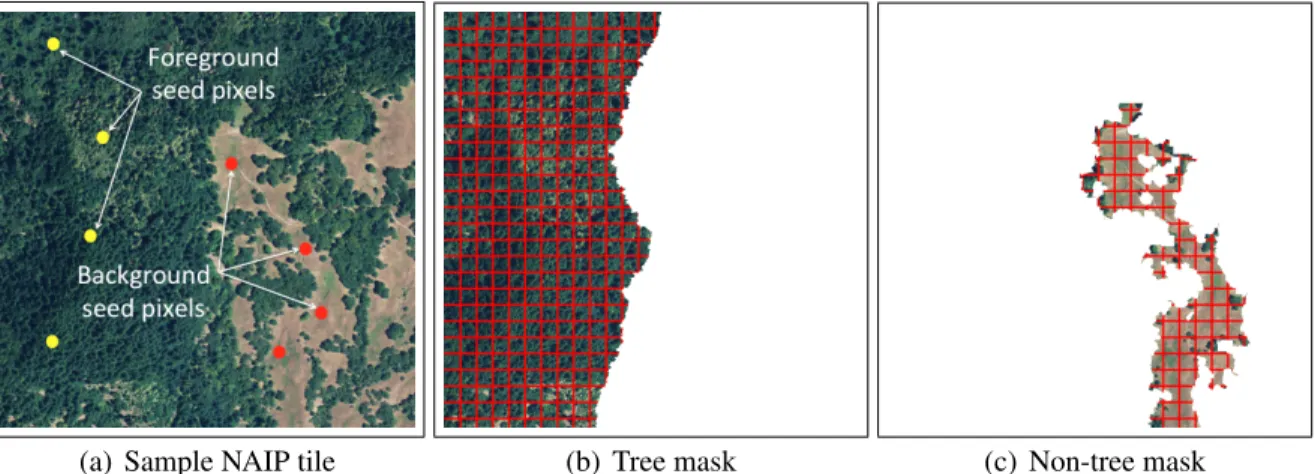
We use an interactive image segmentation tool to extract and label the training samples as well as to re-label misclassified image patches in the online update phase described above. The interactive segmentation module uses a Random Walk based image segmentation algorithm first presented in [42]. In this method, at first a certain number of pixels are labeled as background and foreground seed pixels. These act as seeds for the segmentation algorithm. For any given unlabeled pixel in the original image, a random walk is initialized at the pixel. It is possible to estimate the probability with which a random walk which starts at any unlabeled pixel will reach one of the forground or background seed pixels first. Forkseed pixels, we get ak×1probability vector for each unlabeled pixel, each element of which represents the probability that the random walk starting at that particular pixel reaches the corresponding seed pixel first. Then we can label each pixel as belonging to a specific class based on which element in the probability vector has the highest value. Figure 2.7 shows a sample NAIP tile with tree and non-tree masks generated by the Random walk based segmentation algorithm by selecting a certain number of foreground and background seed pixels corresponding to tree and non-tree areas. The foreground and background seed pixels are marked with yellow and red circles, respectively. The red boxes in Figure 2.7(b) and Figure 2.7(c) represent the training samples extracted from the image which are in turn saved to the training database with the correct label. Note that only complete boxes representing 4×4

training images are saved to the database while the rest are discarded. It is useful to note that the class masks shown in Figure 2.7 are created by manually selecting a certain set of seed pixels. Choosing a different set of seeds can create a different segmentation mask.

2.3.7

Implementation details and the High Performance Computing

Ar-chitecture

We have deployed the abovementioned modules as stand alone on the NASA Earth Exchange (NEX) supercomputing cluster. The deployment was done through QSub routines and the Mes-sage Passing Interface (MPI). The data was accessed through a MySQL database. The NAIP tiles were processed in parallel in the cores of the NASA Earth Exchange High Performance

(43)

Com-(a) Sample NAIP tile (b) Tree mask (c) Non-tree mask

Figure 2.7: A sample NAIP tile with tree and non-tree cover masks generated by the Random Walker Segmentation module by selecting a certain set of foreground and background seed pixels. The small red squares indicate the training samples extracted from the image which are in turn saved to the training database with the correct label. Note that only complete squares representing

4×4training images are saved to the database while the rest are discarded.

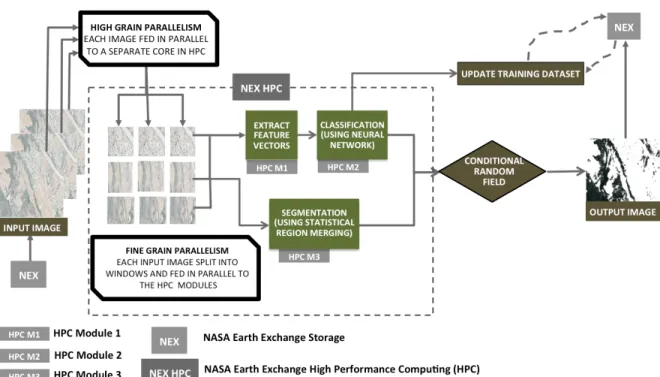
puting (NEX HPC) platform. Each node in the cluster having Harpertown CPUs consists of 8 gigabytes of memory and 8 cores with 3GHz processors per node [111]. In order to process 8 tiles in parallel, one tile per core, the memory requirement per core has to be kept lower than 1 Gigabyte. However, the problem arises with the use of the Statistical Region Merging (SRM) algorithm illustrated in Section 2.3.1. Despite being fast, the algorithm has to store all the indices in memory while sorting them using radix sort as it makes decisions about region boundaries us-ing global scene level image descriptors. This has space complexity of the order ofO(n2₎_{, which} indicates all image gradients in an×nimage, which is of the order of∼3 Gigabytes for a typical NAIP tile. In order to address this memory-performance tradeoff, each image was split intoλ×λ windows and then fed in a pipeline to each core in the HPC node. λwas chosen to be 256 for our experiments, because, higher values led to a higher memory requirement while lower values resulted in a substantial increase of processing time. The current architecture takes a maximum of approximately 4 hours to process each NAIP tile. The details of the architecture are illustrated in Figure 2.8.

(44)

Figure 2.8: High Performance Computing Architecture of our approach.

2.4

Results and Discussion

A rudimentary implementation of our framework produced encouraging results. We chose 1500 image tiles at random covering the following three types of landscapes (1) Densely forested, (2) Fragmented forests, and (3) Urban forested areas. A total of 36000 sampling points were cho-sen at random from the test images - 12000 samples for each land-cover type. The sample vali-dation points are shown in Figure 2.19. The classifier accuracy was measured and averaged over 100 iterations. The results are tabulated in Table 2.4, which shows that our framework produces true positive rates higher than 85% for both densely forested and fragment