Sensor Nework proposeations

A cooperative single target tracking algorithm

using binary sensor networks

Danial Aghajarian, Reza Berangi

Computer Engineering Department,

Iran University of Science and Technology, Iran

Abstract- Sensor networks include large number

of low cost sensor nodes with small processing capabilities that are deployed over an area in an attempt to do interest sensing task. In this paper we examine the role of very simple and noisy sensors for distributed tracking problem that is one of these tasks. We use a proposed binary sensor model, where each sensor’s value is converted reliably to one bit of information only: whether the object is moving toward the sensor or away from it and propose a cooperative distributed algorithm that can be used in real-time tracking and is efficient in power and bandwidth. We show that how an estimator sensor use information from its neighbors to estimate target location more accurately. Our extensive simulations show low error in low density sensor networks.

Key words- Cooperative target tracking, Distributed algorithm, Sensor networks

I. Introduction

Sensor networks include large number of low cost sensor nodes with small processing capabilities that are deployed over an area in an attempt to do interest sensing task. The number of sensor nodes may be on the order of hundreds or thousands. Depending on the application, the number may reach an extreme value of millions [1]. Also the density of the sensor nodes can range from few sensor nodes to few hundred in a region, which can be less than 10 m in diameter [1]. Sensor networks have unique features and limitations that distinguish them from other networks. Large number of sensor nodes, low processing capabilities and power limitation are some of these. Therefore many protocols and algorithms that have been proposed for traditional wireless ad hoc networks cannot be used for sensor networks.

One of sensor network’s application is target tracking that was initially investigated 2002[2,3,4,5,6]. Target tracking has been a classical problem since the early years of electrical systems. In a given field of surveillance interest, there is a target that arises in the field at random location and at random time. The movement of this target follows an arbitrary but

continuous path, and it persists for a random amount of time before disappearing in the field. The target location is sampled at random intervals. The goal of the target tracking problem is to find the moving path for this target in the field. Traditional target tracking systems are based on powerful sensor nodes, capable of detecting and locating targets in a large range and all sensed data were centralized in a powerful computer for running tracking algorithms [7].

With the advances in the fabrication technologies that integrate the sensing and the wireless communication technologies, tiny sensor motes can be densely deployed in the desired field to form a large-scale wireless sensor network. The numbers of sensor nodes are two to three magnitudes greater than those in traditional multisensor systems. On the other hand, each sensor node can have only limited sensing and processing abilities. A target tracking system in this model can have several advantages [7]: 1) the sensing unit can be closer to the target, and thus the sensed data will be of a qualitatively better geometric fidelity; 2) the advances in wireless sensor network techniques will guarantee quick deployment of such a system the sensed data can be processed and delivered within the network, so that the final report about the target is accurate and timely; and 3) with a dense deployment of sensor nodes, the information about the target is simultaneously generated by multiple sensors and thus contains redundancy, which can be used to increase the system’s robustness and increase the accuracy of tracking.

Challenges and difficulties, however, also exist in a target tracking sensor network:

1. Tracking needs collaborative communication and computation among multiple sensors. The information generated by a single node is usually incomplete or inaccurate [7].

2. Each sensor node has very limited processing power. Traditional target tracking methods based on complex signal processing algorithms may not be applicable to the nodes 0 [1] [2].

3. Each node also has tight budget on energy source. Every node cannot be always active in sensing and data forwarding. Thus, all the network protocols for data processing and tracking should consider the impact of power saving mode in each node.

4. The topology of a sensor network may change very frequently [1].

For a target tracking sensor network, the tracking scheme should be composed of two components [7]. The first component is the method that determines the current location of the target. It involves localization as well as the tracing of the path that the moving target takes. The second component involves algorithms and network protocols that enable collaborative information processing among multiple sensor nodes. The goal of this component is to devise techniques for efficient and distributed schemes for collaborations between nodes of a sensor network. Distributed algorithms for detection and tracking of mobile targets are designed within the constraints of various resources (especially power constraints). In this paper we propose a distributed algorithm in the context of a tracking application focused on binary sensors model proposed in [2]. The binary model assumption is that each sensor network node has sensors that can detect one bit of information. This bit shows that whether an object is approaching sensor or moving away from it. We analyze this binary sensor network in the context of a tracking application and derive a tracking algorithm that can be used for real-time tracking in applications with high speed velocity movement. We also show that a binary sensor network in which sensors have only one bit of information do not have enough information content to identify the exact object location but For many applications this accuracy is enough—for example in tracking a flock of birds, a school of fish, vehicle convoy.

The remainder of the article is organized as follows. We discuss related work in the next section. Used binary sensor model for development of algorithm will discuss in section 3. In section 4 and 5 we describe main algorithm and some implementation details. We see simulation result in section 6 and then conclude our article in section 7 and talk about our future work in section 8.

II. Related work

Target tracking is concerned with approximating the trajectory of one or more moving objects based on some partial information, usually provided by sensors. Target tracking is necessary in various domains such as computer vision [8], sensor networks [9], tactical battlefield surveillance, air traffic control, perimeter security and first response to emergencies . A typical example is the problem of finding the trajectory of a vehicle by bearings measurement, which is a technique used by radars. Work in robotics has also considered tracking targets from moving platforms [10].

Several methods for tracking have been proposed. This includes Kalman filter approaches or discretization approaches over the configuration space. A recent method that shows great promise is particle filtering, which is a technique introduced in the field of Monte Carlo simulations. In [2] proposed a binary algorithm based on particle filter approach. The seminal paper in this domain is [12], which states the basic algorithm and properties. Since then many papers have addressed this topic; among the most important are the variance reduction scheme [11] and the auxiliary particle filter [13]. A survey of theoretical results concerning the convergence of particle filter methods can be found in [14].

Probabilistic methods have also been used in robotics for simultaneous localization and mapping (SLAM), in which the robot attempts to track itself using the sensed position of several landmarks. For example, in [15], particle filter techniques were used for localization only when the traditional Kalman filter technique had failed. These algorithms typically assume range and bearing information between the landmarks and tracked vehicle, unlike the very simple sensors considered here.

A distributed protocol for target tracking in sensor networks is developed in [16]. This algorithm organizes sensors in clusters and uses 3 sensors in the cluster toward which the target is headed to sense the target. The target’s next location is predicted using the last two actual locations of the target.

We are inspired by this previous work and use a distributed method in the context of the binary sensor model.

III. Sensor Network model

We assume that the sensor nodes are scattered randomly in a geographical region. Each node is aware of its location. Location’s information can be gathered using an on-board GPS receiver. Absolute location’s information is, however, not needed. Many localizing techniques can be used with varying degree of hardware complexity and accuracy. See, for example,Error! Reference source not found.Error! Reference source not found. . The sensor nodes are stationary in our model; this makes the localization problem somewhat simpler.

We use a binary sensor network model. Each sensor node in this network consists of sensors that can each supply one bit of information only. In this article we assume that the sensor nodes have only one binary sensor that can detect whether the object is approaching or moving away. The detection is performed as follows. Each sensor performs detection

and compares its measurement with a precomputed threshold (e.g., likelihood radio test). If the probability of presence is greater than the probability of absence, also called the likelihood ratio, the detection result is positiveError! Reference source not found.. The model assumes that sensors can identify whether a target is moving away from or towards it

In each step, all sensors that report approaching target to itself form a set that we will call them, plus sensors and we will call sensors that report moving away, minus sensorsError! Reference source not found.. We can formulate these definitions as equation(1) :

{ |

1}

{ |

1}

i i i i

Plus sensors

S s

Minus sensors

S s

=

= +

=

= −

(1)

Where

S

_imeans ith sensor and

s

_i means value of ith sensor.

In Error! Reference source not found. represented some sensor network geometry properties that show the location of the tracked object is outside the convex hull of the plus sensors (we call this convex hall as plus convex hull) and also outside the convex hull of the minus sensors (minus convex hull). We use this property in initialization phase in our algorithm later.

IV.The tracking algorithm

As In this section we describe our tracking algorithm.

A. Algorithm details

Our tracking algorithms make three assumptions. First, for each target that enters the region we suppose its velocity is fixed (

V

_t). For the sake of simplicity we also suppose sensors know this velocity. For example if we deploy some speed detection sensors in the edges of the region, when target enters the region from an arbitrary direction, these sensors can estimate its speed and broadcast it to other sensor nodes. This does not have a heavy communication cost for the network, because the speed detection operation is done only once for each target. Also the number of speed detection sensors is negligible with respect to the number of main

influence the cost of whole sensor network. Our second assumption is that movement of the target in the region is under mild path (at each sensor readings the direction of the tracked object can vary from the previous one with at most

π

/ 6

). We describe later about use of this assumption. The third assumption is that all sensor nodes are time synchronized.

We suppose that when a target enters the range of a sensor, the sensor starts sensing and saving two consecutive sensor reading values. When there is a change in the reading (we call this position the critical point hereafter), the sensor node can estimate the position of the target and broadcast both position and its reading time to the network. Each sensor keeps previous estimation and its time (we call them

1

ˆ

_t

x

₋ and

T

_t−1 respectively). In the following we will discuss and prove that the estimate refers to two different positions located on a circle,

C

_t , centered on the previous target position

x

ˆ

_t−1 with a radius of

t

r

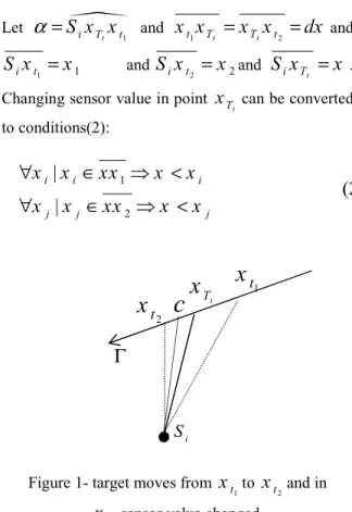
that is target’s displacement between previous estimation and the current one.

Theorem1. Let i be an arbitrary sensor, located at position

S

_i .Also Let

t

₁ and

t

₂be two times so that

1

1

t i

s

= +

and 2

1

t i

s

= −

where 1 2 t t i

and

i

s

s

are

sensor reading’s values at times

1 2

t and t

respectively. Without loss of generality, suppose

t

₁

< <

T

_t

t

₂ and target move on straight line

x x

_{t1 t2}. If

lim

t

₁

− =

t

₂

0

then

T

_t is time that sensor reading value for sensor i change. Then lines

t T i

S x

and 1 2 t t

x x

are perpendicular in point

t

T

x

. Proof.

Let angel between lines

t T i

S x

and 1 2 t t

x x

JJJJJG

α

. Assume by contradiction that

α

≠

90

. Therefore there are two states.

α

>

90

And

α

<

90

. First consider

α

>

90

. In figure 1 we see this state.

Let

n

1 t i T t

S x x

α

=

and 1 t t 2 t T T t

x x

=

x x

=

dx

and 1 1 i t

S x

=

x

and 2 2 i t

S x

=

x

and t i T

S x

=

x

. Changing sensor value in point

t T

x

can be converted to conditions(2): 1 2

|

|

i i i j j j

x x

xx

x

x

x x

xx

x

x

∀

∈

⇒

<

∀

∈

⇒

<

(2)

Figure 1- target moves from

1 t

x

to 2 t

x

and in t T

x

sensor value changed.

In writing these conditions we suppose first target moves toward sensor and then going away it.

n

2

90

90

t t T i

x x S

α

>

⇒

<

And because

x

<

x

₂ then

n

n

2 t t 2

90

i t T i T t

S x x

<

S x x

<

. In 2 t i T t

S x x

+

we have

m

m

2 2 t T

x and x

are less than 90 therefore altitude

line from

S

_i is inside triangle. We suppose this altitude intersect

2 t

T t

x x

at point c (see figure 1). In

t

i T

S cx

+

angel c is 90 and therefore

x

>

S c

_i and this is on the contrary with second condition in(2). Therefore

α

>

90

.

For the case

α

<

90

in the same manner contradict with(2), therefore

α

=

90

.

,

This theorem can be used to locate the target, assuming that a straight line path and a fixed

velocity. Displacement (

d

_t) between two critical points in which the reading values change is calculated from(3).

1

(

)

t t t t

d

=

v T

−

T

₋ (3)

This displacement gives us a circular locus,

C

_t, for the next location,

T

_t, with the center

x

ˆ

_t−1 and the radius

d

_t. On the other hand, we know from theorem1 that the target trajectory and the connecting line between the sensor

S

_i (reporting sensor) and the critical point are perpendicular. These give two possible positions for the target, that are tangent points of the lines from the sensor

S

_i (the reporting sensor) to the circle,

C

_t, as shown in figure 2. We can represent these points as:

l

_t

{ |

l

_{t 1}

}

t i

x

∈

y yS

⊥

y x

−

and y is onC

(4)

Figure 2- Location estimation of target based on theorem1. points x1_t and x2_t can be an estimation for location of target that algorithm calculate middle of these two point on the circle for final estimation of target.

As there is no further information to district between these two points, estimator sensor with cooperative manner can increase accuracy of estimation in each step. By combining data from neighboring sensors, algorithm can reach a tracking

t T

x

x

t1 2 t

x

i

S

Γ

c

result with a resolution higher than that of the individual sensors being used.

In each step, the sensor that estimates position sends a vottingmessage to its neighbors. This message contains two next position locus and id of estimator sensor. Each node after receiving this message, check its readings with these two points and send a new message to estimator node. If each two points have not consistency with its reading that node doesn’t send any message because this condition has not any information for estimation. This is power efficient manner. Also if each two points have consistency with sensor reading, node doesn’t send any message. This is because of power efficiency too. In two remain conditions there is an accepted point and a rejected point and node sends a message to estimator node. This message contains id of sender and accepted point. Estimator node waits for a time out after sending vottingmessage. Then estimate new position according to received messages as follow.

Suppose C1 is number of messages that estimator received and validates x1_t and C2 is number of validation messages for point x2_t then:

• Estimator node choose x1_t as next position x_t if C1-C2>1.

• Estimator node choose x2_t as next position x_t if C2-C1>1.

• Otherwise x_t choose as middle point of x1_t and x2_t on circle

C

_t. This point depict as x_t on figure 2.

New algorithm can be rewrite as below:

0 1 1 0 1 ( ) 1 2 ( , ) ( , 1 , 2 )

1

0

( arg

)

t t t t t t t t t t t t t x V T T x and x oncircle x d sendvottingmessage id x x to neighbers receivevalidationmessage for at

t

y

Initialize

while t

et is in range

y

sensor readingvalue

if y

y then

d

calculate

− − − = −

=

=

=

≠

1 2 1 2 1 2 1 1 t t t _t imeout set C number of messages that validate x set C number of messages thatvalidate x

if C C then set x x = = − > =

2 1 1 2 1 2

( , )

1

t _t t t t t _t elseif C C then set x x else average of x and x as new position on circle end if

set x

broadcast x T

t

t

end if

end while

− > = =

= +

B. Experiments

To evaluate our approach, we implemented our tracking Algorithm in MATLAB and performed simulations. For each point in the plot, we run our algorithm for 200 trajectories and random sensor networks and average results. The Fig. 3 is based on Absolute Mean Error (AME).

Suppose

r(k)

is actual position of the object in time k and

E(k)

is estimation of algorithm AME error model calculated as equation(8).

1

1

( )

( )

n AME k

Error

r k

E k

n

₌

=

∑

−

(5)

Where n is number of location estimations.

Each plot in figure 3 is concern with sensor range. When a sensor range is R, mean that the sensor can detects always the target with distance d that

0.1

d < −R and detects sometimes in ranges

0.1 0.1

R− ≤ ≤ +d R .

The plots in figure 3 show estimation error is sorted with sensor range. This means that sensors

with longer range estimate target location with bigger AME error.

IV.

Conclusions

In this paper we studied a new target tracking algorithm for wireless sensor networks. We assume that node in the networks have sensors that can give one bit of information which distinct abject is approaching or moving away from sensors. We proof

Absolute Mean Error

0 0.01 0.02 0.03 0.04 0.05 0.06 25 36 49 64 81 100 121 144 169 196 225 256 Number of sensors AM E R=0.05 R=0.06 R=0.07 R=0.08 R=0.09 R=0.10

Figure 3 – The plot shows AME error for tracking algorithm. The plot show number of sensors is not influenced accuracy of algorithm hardly. Little decreasing in error is because of initialization phase.

a geometric theorem that gives us conditions for determine object location locus as two points on a circle. We use this property in our tracking algorithm for estimating the target location.

The simulation results show that the accuracy of algorithm is not influenced hardly by number of sensors. This is because in each step location estimation is down only by a sensor node and increasing number of sensors in the field, increase number of estimation (it means that decrease the time between two estimations). Number of sensors influence more, initialization phase of algorithm that cause a little improvement in accuracy. Because this property of algorithm it is well suited for using in low

density sensor network. Using this algorithm in high density sensor networks causes more efficiency in power and bandwidth of network, because algorithm dose not need to activate all sensors for overlapping detection of target at a time.

In the end of our paper we describe some of the open issue that we plan to consider these in our future work.

One important aspect of future work is noise. Real world sensors are influenced by noise. We can incorporate noise in our model by adding a Gaussian variable to the signal strength gradient at sensor and then quantize it as -1, 0 or 1. A 0 reports at a

certain time means that the sensor’s signal strength gradient is below a certain threshold and thus not reliable enough, which can also be regarded as a temporarily shutdown of the sensor. The Gaussian variable ε has zero mean, but its variance should be determined from real data reflecting sensors’ characteristics.

Also in our algorithm we suppose nodes know velocity of object that it is a drawback. Because in some applications knowing velocity is non-realistic assumption although in many application velocity of object is fixed and known or we can estimate velocity with some speed detection sensors in edge of sensor network field.

Another drawback of our algorithm is that can applied to tracking a single object only, although an extension for tracking multiple objects using group management schemes is discussed in our future works

In the near future we will investigate how to add these concepts to our algorithm and how to extend our algorithms to support multiple target tracking. VI. References

[1] Ian F.Akyildiz and Weilian Su, “A survey on Sensor Network”, IEEE Trans. Communication magazine, Vol.40, No.4, pp102-114 2002.

[2] J. Aslam, Z. Butler, V. Crespi, G. Cybenko, and D. Rus, Tracking a moving object with a binary sensor network, Proc. ACM Int. Conf. Embedded Networked Sensor Systems (SenSys), 2003.

[3] R. R. Brooks, P. Ramanathan, and A. M. Sayeed, Distributed target classification and tracking in sensor network, Proc. IEEE, 91(8) (2003).

[4] J. Liu, M. Chu, J. Liu, J. Reich, and F. Zhao, Distributed state representation for tracking problems in sensor networks, Proc. 3rd Int. Symp. Information Processing in Sensor Networks (IPSN), 2004.

[5] K. Mechitov, S. Sundresh, Y. Kwon, and G. Agha, Cooperative Tracing with Binary-Detection Sensor Networks, Technical report UIUCDCS-R-2003-2379, Computer Science Dept., Univ. Illinois at Urbaba — Champaign, 2003.

[6] F. Zhao, J. Shin, and J. Reich, Information-driven dynamic sensor collaboration for tracking applications, IEEE Signal Proces. Mag. (March 2002).

[7] Rajeev Shorey, A. Ananda, Mun Choon Chan and Wei Tsang Ooi, Mobile, wireless and sensor

Networks technology, applications and future directions, a john wiley & sons, INC.,Piblications, pp 173-194 2006.

[8] W.E.L. Grimson, C. Stauffer, R. Romano, and L. Lee. Using adaptive tracking to classify and monitor activities in a site. In Proc. of IEEE Int’l Conf. on Computer Vision and Pattern Recognition, 22– 29,1998.

[9] F. Zhao, J. Shin, and J. Reich. Information-driven dynamic sensor collaboration for tracking applications. IEEE Signal Processing Magazine, 19(2):61–72, March 2002.

[10] Lynne E. Parker. Cooperative motion control for multi-target observation. In Proc. of IEEE International Conf. on Intelligent Robots and Systems, pages 1591–7, Grenoble, Sept. 1997.

[11] P. Clifford, J. Carpenter and P. Fearnhead. An improved particle filter for non-linear problems. In IEE proceedings - Radar, Sonar and Navigation, I46:2–7, 1999.

[12] D. Salmond, N. Gordon and A. Smith. Novel approach to nonlinear/non-gaussian bayesian state estimation. In IEE Proc.F, Radar and signal processing,140(2):107–113, April 1993.

[13] Michael K. Pitt and Neil Shephard. Filtering via simulation: Auxiliary particle filters. Journal of the American Statistical Association, 94(446), 1999. [14] D. Crisan and A. Doucet. A survey of convergence results on particle filtering for practitioners, 2002.

[15] Eduardo Nebot, Favio Masson, Jose Guivant, and Hugh Durrant-Whyte. Robust simultaneous localization and mapping for very large outdoor environments. In Experimental Robotics VIII, 200–9. Springer, 2002.

[16] H. Yang and B. Sikdar, A Protocol for Tracking Mobile Targets using Sensor Networks, Proceedings of IEEE Workshop on Sensor Network Protocols and Applications, 2003.

[17] Nirupama Bulusu, John Heidemann, and Deborah Estrin. GPS-less low cost outdoor localization for very small devices. IEEE Personal Communications, Special Issue on ”Smart Spaces and Environments”, 7(5):28–34, 2000.

[18] K. Whitehouse and D. Culler. Calibration as parameter estimation in sensor networks. In Proceedings of the First ACM International Workshop on Wireless Sensor Networks and Applications(WSNA), pages 59–67, 2002.