Query Language for Biological Databases

(1)

VYSOKÉ U ˇ

CENÍ TECHNICKÉ V BRN ˇ

E

BRNO UNIVERSITY OF TECHNOLOGY

FAKULTA INFORMA ˇ

CNÍCH TECHNOLOGIÍ

ÚSTAV PO ˇ

CÍTA ˇ

COVÝCH SYSTÉM ˚

U

FACULTY OF INFORMATION TECHNOLOGY DEPARTMENT OF COMPUTER SYSTEMS

QUERY LANGUAGE FOR BIOLOGICAL DATABASES

DIPLOMOVÁ PRÁCE

MASTER’S THESIS

AUTOR PRÁCE

TOMÁŠ BAHUREK

AUTHOR

(2)

VYSOKÉ U ˇ

CENÍ TECHNICKÉ V BRN ˇ

E

BRNO UNIVERSITY OF TECHNOLOGY

FAKULTA INFORMA ˇ

CNÍCH TECHNOLOGIÍ

ÚSTAV PO ˇ

CÍTA ˇ

COVÝCH SYSTÉM ˚

U

FACULTY OF INFORMATION TECHNOLOGY DEPARTMENT OF COMPUTER SYSTEMS

DOTAZOVACÍ JAZYK PRO DATABÁZE

BIOLOGICKÝCH DAT

QUERY LANGUAGE FOR BIOLOGICAL DATABASES

DIPLOMOVÁ PRÁCE

MASTER’S THESIS

AUTOR PRÁCE

TOMÁŠ BAHUREK

AUTHOR

VEDOUCÍ PRÁCE

Ing. TOMÁŠ MARTÍNEK, Ph.D.

SUPERVISOR

(3)

Abstrakt

S rapidně stoupajícím množstvím biologických dat stoupá i důležitost biologických databází. U těchto databází je nezbytné objevování znalostí (nalezení spojitostí, které nebyli známé v čase vkládání dat). K získávání znalostí z biologických databází je nutná konstrukce složitých SQL dotazů, což vyžaduje pokročilou znalost SQL a použitého databázového sché-matu. Biologové většinou tyto znalosti nemají, proto je potřeba nástroje, který by poskytl intuitivnějšího rozhrání pro tyto databáze. Tato práce navrhuje ChQL, intuitivní dota-zovací jazyk pro databázi biologických dat Chado. ChQL umožňuje biologům poskládat dotaz za použití pojmů, které dobře znají bez nutnosti znát SQL nebo použité schéma. Tato práce implementuje aplikaci pro dotazování databáze Chado pomocí ChQL. Webové rozhrání provede uživatele procesem zostavení věty jazyka ChQL. Aplikace přeloží tuto větu do SQL dotazu, odešle jej do databáze Chado a zobrazí vrácená data v tabulce. Výsledky jsou vyhodnoceny testováním dotazů na reálných datech.

Abstract

With rising amount of biological data, biological databases are becoming more important each day. Knowledge discovery (identification of connections that were unknown at the time of data entry) is an essential aspect of these databases. To gain knowledge from these databases one has to construct complicated SQL queries, which requires advanced knowledge of SQL language and used database schema. Biologists usually don’t have this knowledge, which creates need for tool, that would offer more intuitive interface for querying biological databases. This work proposes ChQL, an intuitive query language for biological database Chado. ChQL allows biologists to assemble query using terms they are familiar without knowledge of SQL language or Chado database schema. This work implements application for querying Chado database using ChQL. Web interface guides user through process of assembling sentence in ChQL. Application translates this sentence to SQL query, sends it to Chado database and displays returned data in table. Results are evaluated by testing queries on real data.

Klíčová slova

Dotazovací jazyk, Databáze biologických dat, Chado, Gene ontology, Sequence Ontology, Vaadin

Keywords

Query Language, Biological Database, Chado, Gene ontology, Sequence Ontology, Vaadin

Citace

Tomáš Bahurek: Query language for biological databases, diplomová práce, Brno, FIT VUT v Brně, 2015

(4)

Query language for biological databases

Prohlášení

Prohlašuji, že jsem tuto diplomovou práci vypracoval samostatně pod vedením pana Ing. Tomáše Martínka, Ph.D.

. . . . Tomáš Bahurek

May 24, 2015

Poděkování

Ďakujem Ing. Tomášovi Martínkovi, Ph.D. za podnetné rady pri vypracovávaní tejto práce.

c

Tomáš Bahurek, 2015.

Tato práce vznikla jako školní dílo na Vysokém učení technickém v Brně, Fakultě infor-mačních technologií. Práce je chráněna autorským zákonem a její užití bez udělení oprávnění autorem je nezákonné, s výjimkou zákonem definovaných případů.

(5)

List of Figures

2.1 Structure of gene [4] . . . 10

3.1 Summary database schema for UCSC Genome Browser [6] . . . 13

4.1 Modules in Chado and their relationships [8]. . . 19

4.2 Tables in Feature Module [8] . . . 22

4.3 Interbase sequence coordinates [8]. . . 24

4.4 Example of featureloc graph [8] . . . 25

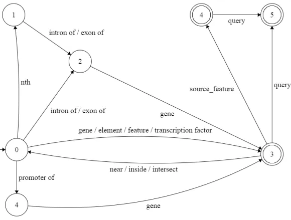
5.1 Finite State Machine accepting ChQL Level 1 . . . 38

6.1 Web interface for creating sentence in ChQL language . . . 50

6.2 Query results in web interface . . . 50

6.3 UML diagram for ChQL Query Builder . . . 53

(8)

List of Tables

2.1 Tags in GFF3 format [4] . . . 11

4.1 Sequence ontology terms in Chado [8] . . . 20

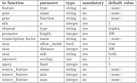
5.1 Parameters of ChQL language . . . 37

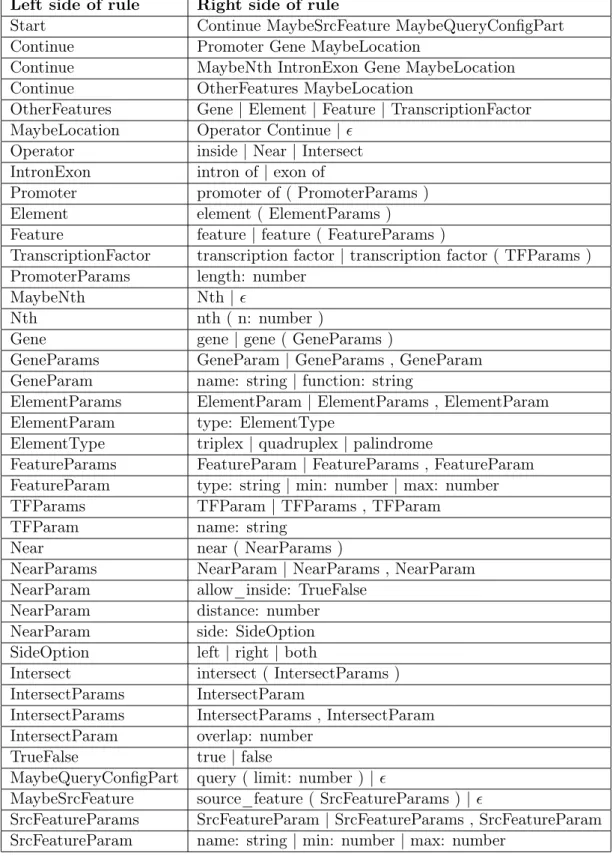
5.2 Grammar for ChQL Level 2 . . . 40

5.3 Words of ChQL with relationship to increasing wid (word id) . . . 41

5.4 Aliases for tables based on context . . . 41

5.5 Near parameters: values of start and end variables . . . 48

7.1 Triplexes in promoter of gene ”C1orf170“ . . . 56

7.2 Quadruplexes near transcription factors . . . 58

7.3 Quadruplexes in first intron of gene . . . 59

7.4 Triplexes in gene ”RERE“ . . . 60

7.5 Types of features in database . . . 61

(9)

Chapter 1

Introduction

Considering the vast amount of available biological data, biological databases are one of the most important tools used by biologists. These databases are usually used for knowledge discovery. They are queried to gain some new information, which was not known at time of data entry.

Typical questions asked by biologists are :

• Which genes have promoters containing specified element (triplex, quadruplex, palin-drome, transcription factor, etc.)?

• How often can be a specified DNA structure (triplex, quadruplex, palindrome, etc.) found near given transcription factor (for example TP53)?

• Which nonB DNA structures are inside gene with specific gene ID (especially in human genome)?

It can be quite complicated to write such queries in SQL, especially for biologists who are often not familiar with this language. In their queries biologists often use terms like promoter, intron, exon, transcription factor and so on. Some of these terms are not exactly identifiable, for example: promoter can have variable length. Sometimes promoter before gene is taken into account, other times promoter before specific transcript is of interest. Adverbs describing positional relationships are ambiguous as well (What is the distance threshold to consider something being near? Does it still count if objects are overlapping as well?). Biologists are often interested, if a specific element exists near other element, if they are overlapping, or if one element is part of other element.

To summarize, there are two problems:

1. Biologists need a more intuitive way to create queries than SQL. 2. Biologists use ambiguous terms in their queries.

This work proposes solution to these problems in form of ChQL. ChQL (Chado Query Language) is a language for querying Biological database Chado. This language uses terms biologists are familiar with, while leaving the unknown technical terms in the background. Wherever possible it uses default values for ambiguous terms with the option of changing them.

Instead of making the user typing words in ChQL, we created a web interface that navigates user through process of assembling sentence in this language. Interface lets user choose next word from the menu, but offers only words that are syntactically correct in

(10)

current context. It also lets user send the query only if current sentence is completed. This is to avoid situation when user makes a typo or syntax error and has to figure out how to fix it. When user completes sentence in ChQL, application translates it to SQL query, which it sends to database server and displays returned results in a table.

This is work contains 8 chapters. Chapter 2 explains gene ontology, sequence ontology and GFF3 file format. Chapter 3 shows some of current database schemas for biological data and querying tools for biological databases. Chapter 4 explains Chado and its most relevant modules. Chapter5proposes design of a language for biological databases including its translation to SQL. Chapter 6 describes implementation of this translation and entire application. Chapter 7evaluates results and performance of queries translated to SQL.

(11)

Chapter 2

Genome Annotation

2.1

Gene Ontology

The Gene Ontology (GO) project [1] is a collaborative effort to address the need for consis-tent descriptions of gene products across databases. Founded in 1998, the project began as a collaboration between three model organism databases: FlyBase (Drosophila), the Sac-charomyces Genome Database (SGD) and the Mouse Genome Database (MGD). The GO Consortium (GOC) has since grown to incorporate many databases, including several of the world’s major repositories for plant, animal, and microbial genomes.

The GO project has developed three structured, controlled vocabularies (ontologies) that describe gene products in terms of their associated biological processes, cellular components and molecular functions in a species-independent manner. There are three separate aspects to this effort: first, the development and maintenance of the ontologies themselves; second, the annotation of gene products, which entails making associations between the ontologies and the genes and gene products in the collaborating databases; and third, the development of tools that facilitate the creation, maintenance and use of ontologies.

The use of GO terms by collaborating databases facilitates uniform queries across all of them. Controlled vocabularies are structured so they can be queried at different levels; for example, users may query GO to find all gene products in the mouse genome that are involved in signal transduction, or zoom in on all receptor tyrosine kinases that have been annotated. This structure also allows annotators to assign properties to genes or gene products at different levels, depending on the depth of knowledge about that entity.

2.2

Sequence Ontology

The Sequence Ontology [4] is a set of terms and relationships used to describe the features and attributes of biological sequence. SO includes different kinds of features which can be located on the sequence. Biological features are those which are defined by their disposition to be involved in a biological process. Examples are binding_site and exon. Biomate-rial features are those which are intended for use in an experiment such as aptamer and

PCR_product. There are also experimental features which are the result of an experiment. SO also provides a rich set of attributes to describe these features such as

”polycistronic“ and

”maternally imprinted“ .

The Sequence Ontologies are provided as a resource to the biological community. They have the following uses:

(12)

• To provide for a structured controlled vocabulary for the description of primary anno-tations of nucleic acid sequence, e.g. the annoanno-tations shared by a DAS server (BioDAS, Biosapiens DAS), or annotations encoded by GFF3.

• To provide for a structured representation of these annotations within databases. Were genes within model organism databases to be annotated with these terms then it would be possible to query all these databases for, for example, all genes whose transcripts are edited, or trans-spliced, or are bound by a particular protein.

• To provide a structured controlled vocabulary for the description of mutations at both the sequence and more gross level in the context of genomic databases.

2.3

GFF3 format

GFF3 is a standard file format for storing genomic features in a text file. GFF stands for Generic Feature Format. The description of GFF 3 format has been summarized from [4].

Description of the Format

GFF3 files are nine-column, tab-delimited, plain text files. Literal use of tab, newline, carriage return, the percent (%) sign, and control characters must be encoded using RFC 3986 Percent-Encoding; no other characters may be encoded. Backslash and other ad-hoc escaping conventions that have been added to the GFF format are not allowed. The file contents may include any character in the set supported by the operating environment, although for portability with other systems, use of Latin-1 or Unicode are recommended.

Note that unescaped spaces are allowed within fields, meaning that parsers must split on tabs, not spaces. Use of the

”+“ (plus) character to encode spaces is deprecated from early versions of the spec and is no longer allowed.

Undefined fields are replaced with the

”.“ character.

Column 1:

”seqid“

The ID of the landmark used to establish the coordinate system for the current feature.

Column 2:

”source“

The source is a free text qualifier intended to describe the algorithm or operating procedure that generated this feature. Typically this is the name of a piece of software, such as ”Genescan“ or a database name, such as ”Genbank.“ In effect, the source is used to extend the feature ontology by adding a qualifier to the type creating a new composite type that is a subclass of the type in the type column.

Column 3:

”type“

The type of the feature (previously called the

”method“ ). This is constrained to be either: • a term from the

”lite“ version of the Sequence Ontology - SOFA

• a term from the full Sequence Ontology - it must be anis_a child ofsequence_feature

(13)

• a SOFA or SO accession number.

The latter alternative is distinguished using the syntax SO:000000.

Columns 4 & 5:

”start“ and ”end“

The start and end coordinates of the feature are given in positive 1-based integer coordinates, relative to the landmark given in column one. Start is always less than or equal to end. For features that cross the origin of a circular feature (e.g. most bacterial genomes, plasmids, and some viral genomes), the requirement for start to be less than or equal to end is satisfied by making end = the position of the end + the length of the landmark feature.

For zero-length features, such as insertion sites, start equals end and the implied site is to the right of the indicated base in the direction of the landmark.

Column 6:

”score“

The score of the feature, a floating point number. As in earlier versions of the format, the semantics of the score are ill-defined. It is strongly recommended that E-values be used for sequence similarity features, and that P-values be used for ab initio gene prediction features.

Column 7:

”strand“

The strand of the feature. + for positive strand (relative to the landmark), - for minus strand, and . for features that are not stranded. In addition, ? can be used for features whose strandedness is relevant, but unknown.

Column 8:

”phase“

For features of type

”CDS“ , the phase indicates where the feature begins with reference to the reading frame. The phase is one of the integers 0, 1, or 2, indicating the number of bases that should be removed from the beginning of this feature to reach the first base of the next codon. In other words, a phase of

”0“ indicates that the next codon begins at the first base of the region described by the current line, a phase of

”1“ indicates that the next codon begins at the second base of this region, and a phase of

”2“ indicates that the codon begins at the third base of this region. This is NOT to be confused with the frame, which is simply start modulo 3.

For forward strand features, phase is counted from the start field. For reverse strand features, phase is counted from the end field.

The phase is REQUIRED for all CDS features.

Column 9:

”attributes“

A list of feature attributes in the formattag=value. Multipletag=valuepairs are separated by semicolons. URL escaping rules are used for tags or values containing the following characters:

”,=;“ . Spaces are allowed in this field, but tabs must be replaced with the %09 URL escape. Attribute values do not need to be and should not be quoted. The quotes should be included as part of the value by parsers and not stripped.

(14)

Figure 2.1: Structure of gene [4]

The Canonical Gene

Below is description of the representation of a protein-coding gene in GFF3. To illustrate how a canonical gene is represented, consider Figure 2.1. This indicates a gene named EDEN extending from position 1000 to position 9000. It encodes three alternatively-spliced transcripts named EDEN.1, EDEN.2 and EDEN.3, the last of which has two alternative translational start sites leading to the generation of two protein coding sequences.

There is also an identified transcriptional factor binding site located 50 bp upstream from the transcriptional start site of EDEN.1 and EDEN2.

Here is how this gene should be described using GFF3:

##g f f−v e r s i o n 3

##s e q u e n c e−r e g i o n c t g 1 2 3 1 1 4 9 7 2 2 8

c t g 1 2 3 . g e n e 1 0 0 0 9 0 0 0 . + . ID=g e n e 0 0 0 0 1 ; Name=EDEN

c t g 1 2 3 . T F _ b i n d i n g _ s i t e 1 0 0 0 1 0 1 2 . + . ID=t f b s 0 0 0 0 1 ; P a r e n t=g e n e 0 0 0 0 1 c t g 1 2 3 . mRNA 1 0 5 0 9 0 0 0 . + . ID=mRNA00001 ; P a r e n t=g e n e 0 0 0 0 1 ; Name=EDEN. 1 c t g 1 2 3 . mRNA 1 0 5 0 9 0 0 0 . + . ID=mRNA00002 ; P a r e n t=g e n e 0 0 0 0 1 ; Name=EDEN. 2 c t g 1 2 3 . mRNA 1 3 0 0 9 0 0 0 . + . ID=mRNA00003 ; P a r e n t=g e n e 0 0 0 0 1 ; Name=EDEN. 3 c t g 1 2 3 . e x o n 1 3 0 0 1 5 0 0 . + . ID=e x o n 0 0 0 0 1 ; P a r e n t=mRNA00003

c t g 1 2 3 . e x o n 1 0 5 0 1 5 0 0 . + . ID=e x o n 0 0 0 0 2 ; P a r e n t=mRNA00001 , mRNA00002 c t g 1 2 3 . e x o n 3 0 0 0 3 9 0 2 . + . ID=e x o n 0 0 0 0 3 ; P a r e n t=mRNA00001 , mRNA00003

c t g 1 2 3 . e x o n 5 0 0 0 5 5 0 0 . + . ID=e x o n 0 0 0 0 4 ; P a r e n t=mRNA00001 , mRNA00002 , mRNA00003 c t g 1 2 3 . e x o n 7 0 0 0 9 0 0 0 . + . ID=e x o n 0 0 0 0 5 ; P a r e n t=mRNA00001 , mRNA00002 , mRNA00003 c t g 1 2 3 . CDS 1 2 0 1 1 5 0 0 . + 0 ID=c d s 0 0 0 0 1 ; P a r e n t=mRNA00001 ; Name=e d e n p r o t e i n . 1 c t g 1 2 3 . CDS 3 0 0 0 3 9 0 2 . + 0 ID=c d s 0 0 0 0 1 ; P a r e n t=mRNA00001 ; Name=e d e n p r o t e i n . 1 c t g 1 2 3 . CDS 5 0 0 0 5 5 0 0 . + 0 ID=c d s 0 0 0 0 1 ; P a r e n t=mRNA00001 ; Name=e d e n p r o t e i n . 1 c t g 1 2 3 . CDS 7 0 0 0 7 6 0 0 . + 0 ID=c d s 0 0 0 0 1 ; P a r e n t=mRNA00001 ; Name=e d e n p r o t e i n . 1 c t g 1 2 3 . CDS 1 2 0 1 1 5 0 0 . + 0 ID=c d s 0 0 0 0 2 ; P a r e n t=mRNA00002 ; Name=e d e n p r o t e i n . 2 c t g 1 2 3 . CDS 5 0 0 0 5 5 0 0 . + 0 ID=c d s 0 0 0 0 2 ; P a r e n t=mRNA00002 ; Name=e d e n p r o t e i n . 2 c t g 1 2 3 . CDS 7 0 0 0 7 6 0 0 . + 0 ID=c d s 0 0 0 0 2 ; P a r e n t=mRNA00002 ; Name=e d e n p r o t e i n . 2 c t g 1 2 3 . CDS 3 3 0 1 3 9 0 2 . + 0 ID=c d s 0 0 0 0 3 ; P a r e n t=mRNA00003 ; Name=e d e n p r o t e i n . 3 c t g 1 2 3 . CDS 5 0 0 0 5 5 0 0 . + 1 ID=c d s 0 0 0 0 3 ; P a r e n t=mRNA00003 ; Name=e d e n p r o t e i n . 3 c t g 1 2 3 . CDS 7 0 0 0 7 6 0 0 . + 1 ID=c d s 0 0 0 0 3 ; P a r e n t=mRNA00003 ; Name=e d e n p r o t e i n . 3 c t g 1 2 3 . CDS 3 3 9 1 3 9 0 2 . + 0 ID=c d s 0 0 0 0 4 ; P a r e n t=mRNA00003 ; Name=e d e n p r o t e i n . 4 c t g 1 2 3 . CDS 5 0 0 0 5 5 0 0 . + 1 ID=c d s 0 0 0 0 4 ; P a r e n t=mRNA00003 ; Name=e d e n p r o t e i n . 4 c t g 1 2 3 . CDS 7 0 0 0 7 6 0 0 . + 1 ID=c d s 0 0 0 0 4 ; P a r e n t=mRNA00003 ; Name=e d e n p r o t e i n . 4

(15)

ID Indicates the ID of the feature. IDs for each feature must be unique within the scope of the GFF file. In the case of discontinuous features (i.e. a single feature that exists over multiple genomic locations) the same ID may appear on multiple lines. All lines that share an ID collectively represent a single feature.

Name Display name for the feature. This is the name to be displayed to the user. Unlike IDs, there is no requirement that the Name be unique within the file.

Alias A secondary name for the feature. It is suggested that this tag be used whenever a secondary identifier for the feature is needed, such as locus names and accession numbers. Unlike ID, there is no requirement that Alias be unique within the file.

Parent Indicates the parent of the feature. A parent ID can be used to group exons into transcripts, transcripts into genes, an so forth. A feature may have multiple parents. Parent can *only* be used to indicate a part_of relationship.

Target Indicates the target of a nucleotide-to-nucleotide or protein-to-nucleotide alignment. The format of the value is

”target_id start end [strand]“ , where strand is optional and may be

”+“ or ”-“ . If the target_id contains spaces, they must be escaped as hex escape %20.

Gap The alignment of the feature to the target if the two are not collinear (e.g. contain gaps). The alignment format is taken from the CIGAR format.

Derives_from Used to disambiguate the relationship between one feature and another when the relationship is a temporal one rather than a purely structural

”part_of“ one. This is needed for polycistronic genes.

Note A free text note.

Dbxref A database cross reference.

Ontology_term A cross reference to an ontology term.

Is_circular A flag to indicate whether a feature is circular.

(16)

Chapter 3

State of the Art

3.1

Biological databases

BioSQL

BioSQL is a generic unifying relational schema for storing sequences and sequence anno-tations from different sources, for instance Genbank or Swissprot. It is also well suited to work with phyloninformatics and phylogenetic trees. BioSQL is meant to be a common data storage layer supported by all the different Bio* projects, Bioperl, Biojava, Biopython, and Bioruby. Entries stored through an application written in, say, Bioperl could be retrieved by another written in Biojava [10].

BioSQL is quite focused and is concerned with: • Sequence

• Sequence annotation • Phylogeny

• Publications

Extension modules extend the core schema and are optional unless specifically needed for storing or retrieving the respective data types the module accommodates. At present, there is one extension module, PhyloDB, for storing phylogenetic trees and taxonomies. Supported RDBMs are at present PostgreSQL, MySQL, Oracle, HSQLDB, and Apache Derby for the core schema. The current release of the BioSQL core schema is v1.0.1. made in August 2008 [11].

Chado

Chado is a relational database schema now being used to manage biological knowledge for a wide variety of organisms, from human to pathogens, especially the classes of information that directly or indirectly can be associated with genome sequences or the primary RNA and protein products encoded by a genome. Biological databases that conform to this schema can interoperate with one another, and with application software from the Generic Model Organism Database (GMOD) toolkit. Chado is distinctive because its design is driven by ontologies. The use of ontologies (or controlled vocabularies) is ubiquitous across the schema, as they are used as a means of typing entities. The Chado schema is partitioned

(17)

into integrated subschemas (modules), each encapsulating a different biological domain, and each described using representations in appropriate ontologies [8].

3.2

Biological querying tools

UCSC Genome Browser

The UCSC Genome Browser was created to provide a graphical viewpoint on the very large amount of genomic sequence produced by the Human Genome Project. The client–server model employed by the UCSC Genome Browser has the advantage to the user of offering access to a very large database of information in a uniform interface with no overhead of importing datasets. The footprint of the data underlying the Genome Browser currently amounts to 7.7 Terabytes (TB) of data in flat files (primarily sequence) and 3.3 TB of tables in a MySQL database (annotations).

Database Structure

Figure 3.1: Summary database schema for UCSC Genome Browser [6]

The construction of a basic genome browser on a new assembly begins with assigning a name. Because assemblies are given a variety of names by the different sequencing centers and no standard nomenclature exists across all organisms, the UCSC database has stan-dardized on a naming system that is internally consistent, though it has evolved. The first assembly for an organism is given a name in the formatgggSss#using the first three charac-ters of the genus and species names, with subsequent assemblies incrementing the number. For example, the cow, Bos taurus, currently has assemblies bosTau2 through bosTau6 on the public site (bosTau1 having been archived).

Two other types of names continue to be used for organisms whose initial assemblies predate the introduction in 2003 of the six-letter naming scheme. Human assemblies are calledhg##, because the database and Genome Browser began when UCSC was generating the human assemblies in-house and the human genome was the only sequence represented. The next several organisms to have browsers were given two-letter names in the format,

gs#, based on scientific names, until the two-character namespace proved inadequate; mouse (Mus musculus) and rat (Rattus norvegicus) are mm#and rn#, respectively.

(18)

Data for each organism are stored in a separate database in the MySQL database system, which is built in a modular design. Each genome assembly has a database named with the genome name as described above (hg#, gs# or gggSss#). This database contains all the assembly-specific tables needed to create a display in the browser graphic, including individual tables for annotation datasets and several tables of metadata describing display parameters, configuration options, etc., specific to the assembly (see Figure3.1).

Several additional databases contain information used by more than one assembly (e.g. data needed to show all the organisms in a pulldown menu). Thus, the hgcentral database contains metadata about the assemblies, including genome name, scientific name, location of the .2 bit file, official assembly name and date and other information. Similarly, the hgFixed database (not shown in Figure 3) contains global information, such as restriction enzyme recognition sites [6].

UCSC Table Browser

The UCSC Table Browser provides text-based access to a large collection of genome assem-blies and annotation data stored in the Genome Browser Database. A flexible alternative to the graphical-based Genome Browser, this tool offers an enhanced level of query support that includes restrictions based on field values, free-form SQL queries and combined queries on multiple tables. Output can be filtered to restrict the fields and lines returned, and may be organized into one of several formats, including a simple tab-delimited file that can be loaded into a spreadsheet or database as well as advanced formats that may be uploaded into the Genome Browser as custom annotation tracks.

The UCSC Table Browser data retrieval tool is built on top of the Genome Browser Database, a set of MySQL relational databases that each store sequence and annotation data for one genome assembly (1). Tables within the databases may be differentiated by whether the data are based on genomic start-stop coordinates or are independent of position. Non-positional tables contain data not tied to genomic location. Some non-positional tables relate internal numeric mRNA IDs to extended information such as author, tissue or keyword. Other ‘meta’ tables contain information about the structure of the database itself or describe external files containing sequence data.

The databases contain optimizations to support range-based queries from the Table Browser and Genome Browser. Smaller tables are indexed on a few critical fields and the data are presorted prior to loading into the database. With larger tables, the data are separated by chromosome into smaller tables, and a binning scheme is implemented on the larger chromosome tables.

In some situations graphical browser may not be optimal tool for working with genomic data. User might wish to view the raw data or examine the relationships between the tables underlying the browser. It is often desirable to filter the display output with greater restrictions than are offered by the Genome Browser, or to output the data in a text-based format that can be imported into other programs.

The UCSC Table Browser provides a powerful and flexible alternative for querying and manipulating the annotation tables within the Genome Browser Database. Using Table Browser form-based or free-form queries, one may quickly and easily extract subsets of the database, in many cases eliminating the need to set up a local copy of the MySQL database. By configuring the tool’s output options, the user can generate a custom annotation track that may be automatically added to the graphical browser session, or create a file in one of several output formats that can be used as input into other programs. The Table Browser

(19)

can also display basic statistics calculated over a selected subset of data.

Basic Data Queries

The Table Browser can be used to retrieve a specific subset of records from a table in a selected genome assembly. The user specifies a position of interest within the assembly (or the keyword ‘genome’ to access data from the entire assembly), selects a table, and then chooses the‘Get all fields’ option. The Table Browser displays the query results in a tab-delimited text format that can be easily downloaded and imported into text editors, spreadsheets and other databases, or may be further processed by the user’s own scripts. For example, a user who is examining alternative splicing in the human genome might be interested in downloading the indices of all mRNA sequences that align to a chromosomal region containing a particular gene. One would set the Table Browser to the gene position, select thechrN_mrna positional table, and then click the Get all fields button. This query produces a tab-delimited list of names and positions of mRNAs that align to the specified location.

Advanced queries

Although basic data retrieval is useful, the real power of the Table Browser lies in the ability to filter and refine queries, intersect query results from different tables and configure the resulting output. These options may be accessed through the Table Browser’s set of ad-vanced query features. The available query formats and output options vary by table. Many apply only to tables in which the data is position-oriented, thus preserving the database distinction between positional and non-positional tables. Position-based tables may be fur-ther differentiated by the types of data they characterize. For example, alignment tables describe a block structure for each element, but other tables may describe only a starting and ending position. Still others may specify translation start and end positions as well as transcription start and end points.

Filtering

The most flexible feature in the Table Browser is its filtering mechanism. The form-based filter provides a straightforward interface for configuring simple SQL-based queries of the data. By default, a Table Browser search retrieves all records for a specified coordinate range or position. Using the filter, the user may set constraints on the values of some or all of the fields within a table to restrict the set of records retrieved from the query range.

The text fields within the filter support wildcard pattern matching and multiple entries. If any word or pattern within the text field matches the value, then the record meets the constraint on that field. Numeric field comparisons support the operators <, >, and != (not equal) and allow comparisons with ranges of numbers.

To satisfy the needs of advanced users who find the form-based filtering options to be insufficient, the Table Browser also supports free-form queries allowing more complex constraints, typically to relate two or more fields within the selected table. These queries, which use SQL ’where’ clause syntax, can combine simple constraints with AND, OR and NOT, using parentheses as needed for clarity. A basic free-form constraint consists of a field name (or an arithmetic expression of numeric field names), a comparison operator and a value.

(20)

For example, when searching for gene models in which a promoter region may be present, the simple free-form query (txStart != cdsStart) on the refGene table will produce a list of genes that have the expected 5’ untranslated region (UTR) upstream sequence. Note that if the strand is negative, this will search for cases of 3’ UTR downstream sequence. In a more complex version of the previous query, (txStart != cdsStart) AND (txEnd != cdsEnd) AND (exonCount = 1) will return a list of single exon genes with both 5’and 3’ flanking UTRs.

Multiple table comparisons

At times one may wish to compare the data between two tables to determine whether any features have positions in common within the genome. The Table Browser provides a simple interface offering the choice of several types of table comparisons based on feature positions. One class of comparisons preserves the gene or alignment structure of the primary table, resulting in output that describes the same type of feature as is shown in that table. Primary table features are kept or discarded based on the amount of positional overlap with features contained in the secondary table. The user controls the query output by specifying the threshold of overlap: any, none or a percentage. For example, one might want to identify all the spliced ESTs that align to a particular region in the Known Genes annotation track. The user would select the location of interest in the Table Browser, choose the chrN_intronEst table, and then proceed to the advanced query options. Intersecting the EST table with the knownGene table results in the desired list. A second class of intersections and unions compares the positions of table features one base position at a time. These queries return only position ranges and do not preserve the structure of the primary table. A base-by-base intersection of two tables will include the base in the output if the nucleotide position is covered by at least one feature of both tables. In a union, the base position need only be covered by the feature of one table.

Retrieving subregions of features

In addition to the SQL constraints on queries, the Table Browser allows the user to specify which subregions of features should be present in the output. For example, someone inter-ested in promoters may want to view the region covered by a gene as well as 5000 additional bases upstream from the 5’ end (or downstream from the 3’ end on the negative strand). The set of available subregion constraints varies among table types. For instance, gene pre-diction tables specify both exon structure and translated region. The user may constrain the output to show upstream and downstream regions, exons, introns, or 5’, 3’, or coding exons. Alternatively, alignment tables, which specify block structure but not translated region, offer only upstream, downstream, blocks or inter-block regions.

Flybase

FlyBase [9], a database of Drosophila genes and genomes, was created in 1992 as a resource for collecting and disseminating Drosophila-related information. The website contains over 2.5 million report pages incorporating data from over 42 000 primary Drosophila research papers and an ever-increasing number of genome-scale projects. As the amount, detail and scope of data in FlyBase has increased, the range of data-retrieval tools has been expanded and improved to ensure that the data in FlyBase are as accessible as possible.

(21)

FlyBase curates a variety of data from published biological literature, including pheno-type, gene expression, interactions (genetic and physical), gene ontology (GO) information and many others. These data are organized in 31 different data-type reports such as the Gene Report or the Allele Report. The range of data provided increases and changes as new types of data become available.

Data-Mining Tools

The tools Flybase provides range from straightforward general search tools and datatype-specific tools to more sophisticated search tools that facilitate wide-range querying of multi-ple data types simultaneously. For straightforward searches, the FlyBase homepage contains the search tool QuickSearch, as well as quick links, via large icons, to a variety of other pop-ular tools, such as BLAST and GBrowse. All tools in FlyBase can be found by using the Tools drop-down menu in our navigation bar, found on every FlyBase page.

QueryBuilder

QueryBuilder (http://flybase.org/.bin/qbgui.fr.html) is a sophisticated web-based search tool that allows combinatorial searching of any fields from any report in FlyBase. Its ad-vanced search capability takes maximum advantage of the data field layout in the underlying Chado database, but its easy-to-use interface means that absolutely no knowledge of this table structure is required. Query segments are built one by one to create complex searches. Data fields are chosen that are specific to a given data type (e.g. the Symbol field from the Gene Report, or the Author field from the Reference Report). After the data type of interest is selected, only appropriate fields are shown as options for each data type, and the fields are presented in similar order and format as in FlyBase report pages to aid nav-igation. Individual query segments can then be combined using Boolean operators (AND, OR and BUT NOT) to build up complex searches. Depending on the fields selected, search criteria can include text strings, CV terms or numbers. Number fields can include calcula-tions and logical funccalcula-tions such as greater than (>) or less than (<), and for many fields an index dictionary is available to allow user to see the most commonly used terms. Wild cards are also allowed, to give user the best chance of carrying out the most appropriate search. An auto-complete function facilitates entry of productive queries. When clicking on the QueryBuilder button on the homepage user is presented with three options: ‘Use a query template’, ‘Import a saved query’ or ‘Build a new query’. For first time users the ‘Use a query template’ option is recommended as a starting point. It contains series of pre-constructed templates covering the most commonly used QueryBuilder queries. These templates are divided into sections according to data type and are fully editable allowing user to adapt them to their individual search criteria.

(22)

Chapter 4

Chado

Chado is a relational database schema that underlies many GMOD installations. It is ca-pable of representing many of the general classes of data frequently encountered in modern biology such as sequence, sequence comparisons, phenotypes, genotypes, ontologies, publi-cations, and phylogeny. It has been designed to handle complex representations of biological knowledge and should be considered one of the most sophisticated relational schemas cur-rently available in molecular biology. The price of this capability is that the new user must spend some time becoming familiar with its fundamentals [8].

4.1

Modules

The Chado schema is built with a set of modules. A Chado module is a set of database tables and relationships that stores information about a well-defined area of biology, such as sequence or attribution.

Arrows are dependencies between modules. Dependencies indicate one or more foreign keys linking modules.

• General - Identifying things within the DB to the outside world, and identifying things from other databases.

• Controlled Vocabulary (cv) - Controlled vocabularies and ontologies • Publication (pub) - Publications and attribution

• Organism - Describes species; pretty simple. Phylogeny module stores relationships. • Sequence - Genomic features and things that can be tied to or descend from genomic

features.

• Map - Maps without sequence

• Genetic - Genetic data and genotypes

• Companalysis - Storage of Computational sequence analysis. The key concept is that the results of a computational analysis can be interpreted or described as a sequence feature.

(23)

Figure 4.1: Modules in Chado and their relationships [8]

4.1.1 General Module

General purpose tables are housed in the module general. The primary purpose of this module is to provide a means of providing data entities with stable, unique identifiers. In Chado, all identifiable data entities have bipartite identifiers, consisting of a dbname plus an accession, together with an optional version suffix.

By convention, these are normally presented using a ’:’ separator. An example of an identifier in this notation would be GO:0008045 or FlyBase:FBgn00000001. In the Chado schema the atomic units are the dbname and the accession, the separator is introduced only in the presentation layer. Each dbname uniquely identifies the authority responsible for a particular ID-space (so there cannot be two GO in any single Chado instance). The accession must be unique within the ID-space. Thus there can be two accessions 0008045, but there can only be one data artefact identified as GO:0008045.

These uniqueness constraints are encoded in the schema, so it is impossible for any Chado relational database instance to violate them.

Each identifier is stored as a row in the dbxref table, with the dbname stored in the db table. Keeping the dbname in a separate db table ensures that the Chado schema retains its commitment to normalization. Entries in other tables can refer to entries in the dbxref table by means of foreign keys.

Note that all stable identifiers are stored in the dbxref table, whether or not they refer to ’external’ data entities. Chado does not have an explicit notion of a data entity being external. Some dbxrefs have further information fully fleshed out in other tables in the database, and others are ’dangling’ dbxrefs.

(24)

4.1.2 Sequence Module

A central module in Chado is the sequence module. The fundamental table within this module is the feature table, for describing biological sequence features. Chado defines a feature to be a region of a biological polymer (typically a DNA, RNA, or a polypeptide molecule) or an aggregate of regions on this polymer. As the term is used here, region can be the entire extent of the molecule, or a junction between two bases. Features can be typed according to an ontology, they can be localized relative to other features, and they can form part-whole and other relationships with other features.

Features

Chado does not distinguish between a sequence and a sequence feature, on the theory that a feature is a piece of a sequence, and a piece of a sequence is a sequence. Both are represented as a row in the feature table.

There are many different types of features. Examples include gene, exon, transcript, regulatory region, chromosome, sequence variation, polypeptide, protein domain and cross-genome match regions. Chado does not have a different table for each kind of feature; all features are stored in the feature table.

Feature types are taken from theSequence Ontology controlled vocabulary (see also Con-trolled Vocabulary module, also known as cv). Types of feature are differentiated using a

type_id column, which is a foreign key to the cvterm table in the cv (ontology) module, described here. This allows us to type features according to the Sequence Ontology. The use of ontologies to type tables gives Chado a subtyping mechanism, which is absent from the standard relational model. For example, SO tells us that mRNA and snRNA are different kinds of transcript. It can be assumed that any reference to genes, exons, polypeptides, SNPs, chromosomes, transcripts and various kinds of RNAs and so on refers to features of that Sequence Ontology type.

A selection of Chado-relevant types from SO are shown below:

SO Term SO id Exon SL:0000025 Intron SL:0000027 mRNA SL:0000037 miRNA SL:0000044 regulatory_element SL:0000052 transcription_factor_binding_site SL:0000054 Table 4.1: Sequence ontology terms in Chado [8]

The Chado feature table has a text-valued column named residues for storing the se-quence of the feature. The value of this column is string of IUPAC symbols corresponding to the sequence of biochemical residues encoded by the feature. This column is optional, because the sequence of the feature may not be known. Even if the sequence of a feature is known, it may not be desirable to store it in the feature table, as it may be possible to infer the sequence from the sequence of other features in the database. For example, exon sequences are generally not stored, as these can trivially be inferred from the sequence of the genomic feature on which the exon is located. In contrast, mRNA and other processed transcript sequences are stored as it is less trivial and more computationally expensive to

(25)

dynamically splice together the mRNA sequence.

It is important to realize that the existence of a row in the feature table does not necessarily imply that the feature has been characterized as a result of genome annotation. It is possible to have features of SO type

”gene“ for genes that have only been characterized through genetic studies, and for which neither sequence nor sequence location is known. This is in contrast to other feature schemas (such as GFF) in which it is not possible to represent features without representing a location in sequence coordinates. This design decision is crucial for the use of Chado as a database for integrating information about the same entity from multiple perspectives.

Because the sequence is stored as a column in the feature table rather than as an inde-pendent table, sequences cannot exist in the absence of a row in the feature table; sequences are dependent upon features. This is in contrast with almost all other genomics schemas that allow independent treatment of sequences and features. This design decision follows for both philosophical and pragmatic reasons. The feature table also contains columns seqlen

and md5checksum, for storing the length of the sequence and the 32-character checksum computed using the MD5 algorithm. The length and checksum can be stored even when the residues column is null valued. The checksum is useful for checking if two or more features share the same sequence, without comparing the entire sequence string.

The existence of these columns means that this table is no longer in third normal form (3NF), which is usually a desirable formal property of relational database. On balance, the utility of these columns outweighs the disadvantages of violating 3NF. In practical terms, it means that the values of the residues, seqlen and md5checksum columns are interdependent and cannot be updated independently of one another.

The feature table has a Boolean valued column,is_analysis, indicating whether this is an annotation or a computed feature from a computational analysis. Annotations are fea-tures that are generated or blessed by a human curator, or in some cases by an integrated genome pipeline (for example, MAKER or DIYA) capable of synthesizing gene models and other annotations from in silico analyses. They constitute the definitive version of a partic-ular feature, in contrast to the features generated by gene prediction programs and sequence similarity searches such as BLAST.

The feature table has adbxref_idcolumn that refers to a global, stable public identifier for the feature. This column is optional, because not all classes of features have such identifiers for example, features resulting from gene predictions and BLAST HSP features may be less stable and thus lack public identifiers. It is recommended that most annotated features have dbxref_ids. The organism_id column refers to a row in the organism table (defined in the organism module). This column is mandatory if the feature derives from a single organism.

Names of Features

The name and uniquenamecolumns allow features to be labelled. The namecolumn is op-tional, but it is recommended that all annotated features (as opposed to those that arise from purely computational methods) have names. The name should be a simple, concise, human-friendly display label (such as a gene or gene product symbol, as defined by the nomenclature rules of governing the organism). User interface software (such as GBrowse and Apollo) can use the name column for labelling feature glyphs in user displays. Unique-ness of name within any particular organism or genome project is a desirable characteristic, but is not enforced in the schema, since there are occasions where name clashes are

(26)

unavoid-able. In contrast, the uniquename column is required, and guaranteed to be unique when taken in combination with organism_id and type_id. This is enforced by a constraint in the relational schema. The unique name may be human-friendly (for example, it can be the same as the name); however, it is not guaranteed to be so, and in general should not be displayed to the end user. Its use is mainly as an alternate unique key on the table .

The unique name normally conforms to some naming rule. These rules may vary across chado instances, but they should all guarantee the uniqueness of the uniquename,

organism_id,type_id triple.

(27)

Feature Synonyms

In addition to having a name or symbol, it is common for referencing features such as genes to have multiple synonyms or aliases. These synonyms may exist due to different publications referring to the same gene with different symbols, or because one gene was once believed to be two or more separate genes. A common curation operation on genes is splitting and merging, which results in the creation of synonyms.

This is modelled in Chado with a synonym table and a feature_synonymlinking table; thus multiple features can potentially share the same, and a single feature can be have multiple synonyms. Use of a synonym in the literature is indicated with a pub_id foreign key referencing the pub table (see the publications module), indicating historical provenance for the use of a synonym.

Feature synonyms are found by joining to feature_synonymand synonym. Below is an example query to find gene by name or synonym:

SELECT f e a t u r e _ i d FROM f e a t u r e

WHERE name = ’ name␣ o f ␣ i n t e r e s t ’

UNION SELECT f e a t u r e _ i d

FROM feature_synonym f s , synonym s

WHERE f s . synonym_id = s . synonym_id

AND s . name = ’ name␣ o f ␣ i n t e r e s t ’

AND f s . i s _ c u r r e n t ;

Feature Locations

Features can potentially be localized using a sequence coordinate system. A relative lo-calization model is used, so all feature lolo-calizations must be relative to another feature. Some features such as those of type chromosome are not localized in sequence coordinates. Locations are stored in the featureloc table, also part of the sequence module. Other non-sequence oriented kinds of localization (such as physical localization from in situ ex-periments, or genetic localizations from linkage studies) are modelled outside the sequence module (for example, in the expression module or map module).

A feature can have zero or more featurelocs, although it will typically have either one (for localized features for which the location is known) or zero (for unlocalized features such as chromosomes, or for features for which the location is not yet known, such as a gene discovered using classical genetics techniques). Features with multiple featurelocs will be explained later.

A featureloc is an interval in interbase sequence coordinates (see figure), bounded by the fmin and fmax columns, each representing the lower and upper linear position of the boundary between bases or base pairs, with directionality indicated by the strand column. Interbase coordinates were chosen over the more commonly used base-oriented coordinate system because they are more naturally amenable to the standard arithmetic operations that are typically performed upon sequence coordinates. This leads to cleaner and more efficient database coding logic that is arguably less prone to errors. Of course, interbase coordinates are typically transformed into the more common base-oriented system used by BLAST reports and so forth prior to presentation to the end-user.

The relational schema includes a constraint which ensures that fmin != fmax is always true, and any attempt to set the database in a state which violates this will flag an error.

(28)

As mentioned previously, a featureloc must be localized relative to another feature, in-dicated using the srcfeature_idforeign key column, referencing the feature table. There is nothing in the schema prohibiting localization chains; for example, locating an exon rel-ative to a contig that is itself localized relrel-ative to a chromosome (see figure). The majority of Chado database instances will not require this flexibility; features are typically located relative to chromosomes or chromosomes arms. Nevertheless, the ability to store such local-ization networks or location graphs can be useful for unfinished genomes or parts of genomes such as heterochromatin, in which it is desirable to locate features relative to stable contigs or scaffolds, which are themselves localized in an unstable assembly to chromosomes or chro-mosome arms. Localization chains do not necessarily only span assemblies protein domains may be localized relative to polypeptide features, themselves localized to a transcript (or to the genome, as is more common). Chains may also span sequence alignments.

Figure 4.3: Interbase sequence coordinates [8]

The Feature Location Graph

A featureloc graph (LG) can be defined as being a set of vertices and edges, with each feature constituting a vertex, and each featureloc constituting an edge going from the parent

feature_idvertex to the srcfeature_id vertex. The node is labeled with column values from the feature table, and the edge is labeled with column values from the featureloc table. The LG is not allowed to contain cycles, it is a directed acyclic graph (DAG). This includes self-cycles - no feature may be localized relative to itself.

The roots of the LG are the features that do not have featureloc rows, typically chromo-somes or chromosome arms, although LG roots may also be unassembled contigs, scaffolds or features for which sequence localization is not yet known (such as genes discovered through classical genetics techniques). The leaves of the LG are any features that are not present as asrcfeature_idin any featurelocs row typically the bulk of features, such as genes, exons, matches and so on. The depth of a particular LG g, denoted D(g), is the maximum number of edges between any leaf- root pair. As has been previously noted, many Chados will have LGs with a uniform depth of 1. Such LGs are said to be simple and the features within them are said to be singletons. The maximum depth of all LGs in a particular database instance i is denoted LGDmax(i).

The schema does not constrain the maximum depth of the LG. This flexibility proves use-ful when applying Chado to the highly variable needs of multiple different genome projects; however, it can lead to efficiency problems when querying the database. It can also make it more difficult to write software to interoperate with the database, as the software must take into account different contingencies. We can solve this problem by collapsing the LG, in which a graph of arbitrary depth is flattened to a depth of 1, transforming or

(29)

project-Figure 4.4: Example of featureloc graph [8]

ing featurelocs onto the root features (typically chromosomes or chromosome arms). The original featurelocs are left unaltered in the database, and additional redundant featurelocs between leaf and root features are added to the database. These new featurelocs are known as inferred featurelocs. In the schema inferred featurelocs are differentiated from direct fea-turelocs using the locgroup column. Direct (non-inferred) localizations are indicated by the locgroup column taking value 0, and transitive localizations are indicated by this column having value !0.

The terminology used above can be used to define specifications for applications intended to interoperate with the database. Certain kinds of features have paired locations. These include hits and high-scoring-pairs (HSPs) coming from sequence search programs such as BLAST, and syntenic chromosomal regions. These kinds of features have two featurelocs (in contrast to the usual 1) one on the query feature and one on the subject (hit) feature. We differentiate the two featurelocs with the rank column. A rank of 0 indicates a location relative to the query (as is the default for most features), and a rank of 1 indicates a location relative to the subject (hit) feature.

For multiple alignments (e.g. CLUSTALW results), this scheme is extended to un-bounded ranks [0..n], with arbitrary ordering. Alignments are stored in the residue info column. CIGAR format is used for pairwise alignments.

Multiple featurelocs may also be required for features of type

”sequence variant“ (SO:0000109), indicating points or extents which vary between reference and non-reference sequences. From a modelling standpoint, variants are conceptually similar to alignments; with variants we are noting a difference as opposed to a similarity. Here a rank of zero indicates the wild-type (or reference) feature and a rank of one or more indicates the variant (or non-reference) feature, with the residue info column representing the sequence on wild-type and variant. A featureloc is uniquely identified by the feature_id, rank, locgroup

(30)

triple. This means that no feature can have more than one featureloc with the same rank and locgroup. In other words, rank and locgroup uniquely identify a featureloc for any particular feature.

Feature Coordinates

Features are located relative to other features using the featureloc table rows. Features can be located on more than one sequence. For example, a BLAST hit HSP can be a feature of both the query and target sequences. To locate a feature, create a featureloc record with:

• srcfeature_id= the id of the sequence on which the feature is being located • feature_id= the id of the feature being located

• strandis 1 for the positive strand, -1 for the negative, and 0 for both or indifferent. • fmin,fmax– the minimum and maximum coordinates of the interval

• is_fmin_partial, is_fmax_partial = true if needed to indicate that the sequence is incomplete (e.g. for ESTs or EST assemblies which are known to not go all the way to the 3’ or 5’ end.)

• phase= 0, 1, or 2 – denotes phase of first base pair in a nucleotide feature with respect to a source protein, or the offset of the first nucleotide in its codon.

• rank, locgroup – these are used to organize groups of feature locations and can be ignored in simple cases (the details are discussed below).

Multiple Locations for a Feature

The ability to have multiple locations for a feature has many uses. For example one can locate a SNP, exon, or protein motif on the genome, on a transcript, and on a protein. A region of similarity between two sequences (HSP) can be located on both of them, so if either is viewed the

”hit“ is visible.

Difference Between the Chado Location Model and Other Schemas

There is a crucial difference between the Chado location model and the sequence location model used in other schemas, such as GFF, GenBank, BioSQL, or BioPerl.

First, Chado is the only model to use the concept of rank and locgroup. Second, and perhaps more important, all these other models allow discontiguous locations (also known as ”split locations“ ). These will be familiar to anyone who has inspected GenBank annotated DNA records for an organism that has introns within the transcripts; the transcript location is modelled as a sequence of non-contiguous intervals on the genome. The interval represents the location of an exon. For example:

/ g e n e="Acph"

CDS j o i n ( 9 1 4 . . 1 0 6 3 , 1 1 4 3 . . 1 2 4 1 , 1 2 9 7 . . 1 5 3 6 , 1 6 0 5 . . 2 0 5 4 , 2 6 6 7 . . 2 9 2 5 , 3 0 6 3 . . 3 1 7 2 )

Although Chado allows a feature to have multiple locations, this is only with variable rank and locgroup and this is enforced by a uniqueness constraint in the relational schema. We made a conscious decision to avoid discontiguous locations, because the extra degree of

(31)

freedom this affords results in either redundancies or ambiguities. Redundancies arise when exons are stored in addition to a discontiguous transcript, and ambiguities arise by virtue of the fact that explicit representation of the exons may be seen as optional. Ambiguities are undesirable as it makes it harder for databases to interoperate. The omission of discon-tiguous locations does not restrict the expressive capacity of Chado in any way, because any discontiguous location can be modelled as a collection of features with contiguous locations. For example, a transcript with a discontiguous location can be modelled as a collection of exons with contiguous featurelocs, and a transcript with a single contiguous featureloc representing the outer boundaries defined by the outermost exons.

Feature Rank

The rank field is used when a feature has more than 1 location, otherwise the default rank value of 0 is used. Some features have two locations, for example BLAST hits and HSPs: one location on the query, rank = 0, and one location on the subject, rank = 1.

Extensible Feature Properties

The feature table has a fairly limited set of columns for recording feature data. For example, there is no anticodon column for recording the RNA triplet for the adapter in a tRNA feature (all feature types, including tRNAs, are recorded as rows in the feature table). If we were to add columns such as anticodon then the number of columns in the table would become very large and difficult to manage; most would end up being nullable (for example, anticodon does not apply to non-tRNA features). This is because different organisms, different types of feature and different projects have differing needs regarding what extra data should be attached to any one feature. How then are we to attach both biologically relevant and project specific data to features?

Chado solves this by using an extensible mechanism for attaching attribute-value pairs to features via the featureprop table. Thefeatureprop.type_idforeign key column references a property in the Sequence Ontology. The value text column stores the value filler for that property. Sets or lists of values for any property can be stored in the featureprop table, differentiated by the value of the rank column. Provenance for the featureprop assignment is stored using the featureprop_pub table in the publications module, allowing multiple publications to be associated with any one assignment.

Because featureprop values can be of an arbitrary size, they are modelled using a SQL TEXT type. This has some disadvantages from a query efficiency perspective.

Numeric values cannot be indexed correctly, and sorting the results of a query can only be done via a SQL casting operation, or in software outside of the database management system, either of which may result in poorer performance. This is one of several areas in Chado where performance has been traded in favour of a simpler, more abstract and generic model.

Linking Features to External Databases

Public database identifiers are stored in the dbxref table, which holds the database name, the accession number, and an optional version number. Note that this table holds accession numbers published internally by the Chado instance as well as by other databases. A feature can have a primary dbxref, which is linked directly from the feature table. It can also have additional secondary dbxref’s linked via feature_dbxref. A feature need not

(32)

have a primary dbxref; e.g. computed features may be considered “lightweight” and not assigned accession numbers. Some groups may wish to set up a trigger to automatically assign primary dbxrefs to features of types that are locally accessioned; a sample trigger is provided with the schema.

Feature Annotations

Detailed annotations, such as associations to Gene Ontology (GO) terms or Cell Ontology terms, can be attached to features using the feature_cvterm linking table. This allows multiple ontology terms to be associated with each feature.

Provenance data can be attached with the feature_cvtermpropand

feature_cvterm_dbxrefhigher-order linking tables. It is up to the curation policy of each individual Chado database instance to decide which kinds of features will be linked using

feature_cvterm. Some may link terms to gene features, others to the distinct gene products (processed RNAs and polypeptides) that are linked to the gene features.

Annotations for existing features can also go into the featureprop table using the Chado

feature_propertyontology (defined inchado/load/etc/feature_property.obo) and the comment or description terms as appropriate. The purpose of the feature property ontology (and the relatedchado/load/etc/genbank_feature_property.obofile) is to capture terms that are likely to appear in GFF or GenBank sequence files. In theory there is no overlap between these ontologies and the Sequence Ontology.

Relationships Between Features

Biological features are inter-related; exons are part of transcripts, transcripts are part of genes, and polypeptides are derived from messenger RNAs. Relationships between individ-ual features are stored in thefeature_relationshiptable, which connects two features via the subject_id and object_id columns (foreign keys referring to the feature table) and a type_id (a foreign key referring to a relationship type in an ontology, either SO, or the OBO relationship ontology, OBO-REL, indicating the nature of the relationship between subject and object features.

The core relationships between features are part-whole (part_of) or temporal

(derives_from). Subject and Object describes the linguistic role the two features play in a sentence describing the feature relationship. In English, many sentences follow a subject, predicate, object syntax, and word order is important. To say that ”exons are part of tran-scripts” is the correct way to describe a typical biological relationship. To say ”transcripts are part of exons” is either grammatically or biologically incorrect.

We use this same terminology (which comes from RDF) again in the cv module. The collection of features and feature relationships can be considered as vertices and edges in a graph, known as the Feature Graph (FG). Example feature graphs are shown above and in the Introduction to Chado.

The FG is independent of the LG and in general the FG and the LG should have no edges in common. If there is a featureloc connecting two features, then the addition of a feature relationship between these same two features is redundant. The FG is required in order to query the database for such things as alternately spliced genes, exons shared between transcripts, etc.

Although the chado schema admits any FG, certain configurations are biologically mean-ingless, and should not be used. The FG can be constrained by the Sequence Ontology. Standardized FG structures are required for complex applications to be interoperable.

(33)

Unlike the LG, the FG may be cyclic, although cycles in the FG are not common. The subset of the FG corresponding to certain kinds of relationship may be acyclic for example, the subset of the FG connecting parts with wholes via part of must be acyclic.

Compliance

Chado uses a layered model - this is tried and tested in software engineering. Some generic software can be targeted at the lower layers and be guaranteed to work no matter what. Other more specific software needs a more tightly defined rigorous model and should be targeted at the upper layers.

We require validation software and more formal or computable descriptions of these layers and policies - for now natural language descriptions will have to suffice.

Chado Compliance Layers Proposal for levels of compliance.

Level 0: Relational Schema Level 0 conformance basically means the schema is adhered to. Obviously, this is enforced by the DBMS.

Level 1: Ontologies Level 1 conformance is minimal conformance to SO - all fea-ture.types must be SO terms, and all feature relationship.types must be SO relationship types.

Level 2: Graph Level 2 conformance is graph conformance to SO - all feature relation-ships between a feature of type X and Y must correspond to relationship of that type in SO; for example, mRNA can be part of gene, but mRNA can not be part of golden path region. [more detailed/formal explanation to come]. In practice Level 2 conformance may be undesirable, we may need to make modifications to SO. Orthogonal to these layers are various additional policy decisions. Some of these are more tolerant of non-conformance than others. (there is also some overlaps with levels 1 and 2).

4.1.3 CV Module

This module is for controlled vocabularies (CVs), semantic networks and ontologies, de-pending on which terminology you prefer. It is intended to be rich enough to encapsulate anything in the Gene Ontology (GO) or OBO family of ontologies. The schema reflects the data model of OBO and of the OBO Edit tool currently used by these projects. This module is also intended to be extensible to richer formalisms such as OWL (Ontology Web Language), but this is outside the current requirements. The schema is similar to the GO database schema, which was also developed by one of the Chado designers.

Overview

An ontology, or controlled vocabulary (CV) is a collection of classes (or concepts or terms, depending on your terminology) with definitions and relationships to other classes. Each class (a word or phrase) can only appear once in a controlled vocabulary and has a defined meaning within that vocabulary. The controlled vocabularies are chosen so that the contents do not overlap; if the same text string is used to describe two different concepts in two different CVs, these are distinct classes. These terms are housed in the cvterm table in the

(34)

Chado schema. CVterms are related to one another via cvter_relationship. This can be thought of as a graph, or semantic network. The relationship types (the labels on the arcs of the graph) are also stored in the cvterm table. The relationship types are extensible, but the type is a (subtyping relationship) is assumed to be present; many OBO ontologies use the part of relationship, and GO also uses the regulates relation. Relationship types also come from a controlled vocabulary, the OBO Relation Ontology. The cvterm_relationship can be thought of as specifying sentences about the cvterms. These sentences have 3 parts - a subject term, an object term, and a verb or type. For example in the phrase

”an exon is part of a transcript“ the subject of the sentence is

”exon“ and the object is ”transcript“ . If you prefer to think of it as a directed graph), then you can think of the subject as the child node, and the object as the parent node.

Associating features to cvterms

This module is used by most of the Chado modules. But it is useful to describe here how this module would be used in the context of the sequence module. It is often desired to attach cvterms to features. One example is typing features with SO - this is central to the sequence module. Each feature has one primary type, stored in featuretype_id. We can also attach an arbitrary number of non-primary cvterms to a feature. For example, we may want to attach GO annotations to gene or protein features. We may also want to attach phenotypic terms to gene features (although the preferred way to do this is via a genotype using the genetics module).

Complex annotations

The s