Irregular Repeat–Accumulate Codes
1Hui Jin, Aamod Khandekar, and Robert McEliece
Department of Electrical Engineering, California Institute of Technology
Pasadena, CA 91125 USA
E-mail:
{
hui, aamod, rjm
}
@systems.caltech.edu
Abstract: In this paper we will introduce an ensemble of codes calledirregular repeat-accumulate
(IRA) codes. IRA codes are a generalization of the repeat-accumluate codes introduced in [1], and as such have a natural linear-time encoding algorithm. We shall prove that on the binary erasure channel, IRA codes can be decoded reliably in linear time, using iterative sum-product decoding, at rates arbitrarily close to channel capacity. A similar result appears to be true on the AWGN channel, although we have no proof of this. We illustrate our results with nu-merical and experimental examples.
Keywords: repeat-accumulate codes, turbo-codes, low-density parity-check codes, iterative decoding.
1.
INTRODUCTION
With the hindsight provided by the past seven years of research in turbo-codes and low-density parity-check codes, one is tempted to propose the follow-ing problem as the final problem for channel codfollow-ing researchers: For a given channel, find an ensemble of codes with (1) a linear-time encoding algorithm, and (2) which can be decoded reliably in linear time at rates arbitrarily close to channel capacity. For turbo-codes, both parallel and serial, (1) holds, but according to the recent work by Divsalar, Dolinar, and Pollara [7], on the AWGN channel there ap-pears to be a gap, albeit usually not a large one, between channel capacity and the iterative decod-ing thresholds for any turbo ensemble. For LDPC codes, the natural encoding algorithm is quadratic in the block length, and from the work of Richard-son and Urbanke [2] we know that for regular LDPC codes, on the binary symmetric and AWGN channels there is a gap between capacity and the iterative de-coding thresholds. On the positive side, however, Luby, Shokrollahi et at. [3], [4], [8], have established the remarkable fact that on the binary erasure chan-nel irregular LDPC codes satisfy (2). Recent work by Richardson, Shokrollahi and Urbanke [5] shows 1This paper is to be presented at the Second International Conference on Turbo Codes, Brest, France, September 2000. This research was supported by NSF grant no. CCR-9804793, and grants from Sony, Qualcomm, and Caltech’s Lee Center for Advanced Networking.
that on the AWGN channel, irregular LDPC codes are markedly better than regular ones, but whether or not they can reach capacity is not yet known. In summary, as yet there is no known noisy channel for which the final problem has been solved, although re-searchers are very close on the AWGN channel and extremely close on the binary erasure channel.
In this paper, we will introduce a promising class of codes calledirregular repeat-accumulatecodes, which generalizes the repeat-accumulate codes of [1]. After defining the codes in Section 2, and observing that they have a simple linear-time encoding algorithm, in Section 3, using the powerful Richarson-Urbanke method [2], we will prove rigorously that IRA codes solve the final problem for the binary erasure chan-nel. In Section 4, we will discuss, less rigorously, the performance of IRA codes on the AWGN chan-nel, and show that their performance is remarkably good.
2.
DEFINTION OF IRA CODES
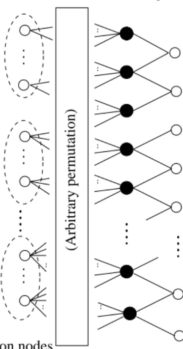
Figure 1 shows a Tanner graph of an IRA code with parameters (f1, . . . , fJ;a), wherefi≥0,
ifi=
1 anda is a positive integer. The Tanner graph is a bipartite graph with two kinds of nodes: variable nodes (open circles) and check nodes (filled circles). There arekvariable nodes on the left, called informa-tion nodes; there are r= (kiifi)/a check nodes;
and there are r variable nodes on the right, called parity nodes. Each information node is connected to a number of check nodes: the fraction of informa-tion nodes connected to exactlyi check nodes isfi.
Each check node is conected to exactlyainformation nodes. These connections can made in many ways, as indicated in Figure 1 by the “arbitrary permuta-tion” of theraedges joining information nodes and check nodes. The check nodes are connected to the parity nodes in the simple zigzag pattern shown in the figure.
If the “arbitrary permutation” in Figure 1 is fixed, the Tanner graph represents a binary linear code withkinformation bits (u1, . . . , uk) andrparity bits
(x1, . . . , xr), as follows. Each of the information bits
is associated with one of the information nodes; and each of the parity bits is associated with one of the
Parity nodes Check nodes (all have left degree a)
Information nodes (fi = fraction of nodes of degree i) f2 f3 fJ x1 x2 xr (Arbitrary permutation)
Figure 1: Tanner graph for IRA code with parame-ters (f1, . . . , fJ;a).
parity nodes. The value of a parity bit is determined uniquely by the condition that the mod-2 sum of the values of the variable nodes connected to each of the check nodes is zero. To see this, let us convention-ally set x0 = 0. Then if the values of the bits on
theraedges coming out of the permutation box are (v1, . . . , vra), we have the recursive formula
xj=xj−1+ a
i=1
v(j−1)a+i, (1)
forj= 1,2, . . . , r. This is in effect the encoding algo-rithm, and so ifais fixed andn→ ∞, the encoding
complexity isO(n).
There are two versions of the IRA code in Fig-ure 1: thenonsystematicand thesystematicverisons. The nonsystematic version is an (r, k) code, in which the codeword corresponding to the information bits (u1, . . . , uk) is (x1, . . . , xr). The systematic version
is a (k+r, k) code, in which the codeword is (u1, . . . , uk;x1, . . . , xr).
The rate of thenonsystematic code is easily seen to be Rnsys= a iifi , (2)
whereas for the systematic code the rate is
Rsys= a a+iifi
(3)
For example, the original RA codes are nonsys-tematic IRA codes with a = 1 and exactly one fi
equal to 1, sayfq = 1, and the rest zero, in which
case (2) simplifies to R = 1/q. (However, in this paper we will be concerned almost exclusively with systematic IRA codes.)
In an iterative sum-product message-passing de-coding algorithm, all messages are assumed to be log-likelihood ratios, i.e., of the formm= log(p(0)/p(1)). The outgoing message from a variable node u to a check nodev represents information aboutu, and a message from a check node u to a variable node v
represents information about u. Intially, messages are sent from variable nodes which represent trans-mitted symbols.
The outgoing message from a nodeuto a nodev
depends on the incoming messages from all neighbors
wofuexceptv. Ifuis a variable message node, this outgoing message is
m(u→v) =
w=v
m(w→u) +m0(u), (4)
wherem0(u) is the log-likelihood message associated
withu. ( Ifuis not a codeword node, this term is ab-sent.) Ifuis a check node the corresponding formula is [10] tanhm(u→v) 2 = w=v tanhm(w→u) 2 . (5)
3.
IRA CODES ON THE BINARY
ERASURE CHANNEL
The sum-product algorithm defined in equations (4) and (5) simplifies considerably on the binary erasure channel (BEC). The BEC is a binary input channel with three output symbols, a 0, a 1 and “erasure.” The input symbol is received as an erasure with prob-ability p and is received correctly with probability 1−p. It is important to note that no errors are ever made on this channel.
It is not difficult to see that the messages defined in (4) and (5) can assume only three values on the BEC, viz. +∞, −∞or 0, corresponding to a vari-able value 0, 1, or “unknown.” No errors can occur during the running of the algorithm; if a message is ±∞, the corresponding variable is guaranteed to be 0 or 1, respectively. The operations at the nodes in the graph given by eqns (4) and (5) can be stated much more simply and intutively in this case. At a variable node, the outgoing message is equal to any non-erasure incoming message, or an erasure if all incoming messages are erasures. At a check node, the outgoing message is an erasure if any incoming message is an erasure, and otherwise is the binary sum of all incoming messages.
3.1.
Notation
In this section and the next, it will be convenient to use a slightly different representation for an IRA code than the one used in Section 2. Firstly, we will begin with the assumption that the degrees of both the information nodes and the check nodes are non-constant, though we will soon restrict attention to the “right-regular” case, in which the check nodes have constant degree.
Secondly, letλi be the fraction ofedgesbetween
the information and the check nodes that are adja-cent to an information node of degree i, and let ρi
be the fraction of such edges that are adjacent to a check node of degree i+ 2 (i.e. one which is ad-jacent to i information nodes). We will use these edge fractions λi and ρi to represent the IRA code
rather than the corresponding node fractions. We defineλ(x) =iλixi−1andρ(x) =
iρixi−1to be
the generating functions of these sequences. The pair (λ, ρ) is called adegree distribution. It is quite easy to convert between the two representations. We demon-strate the conversion with the information node de-grees. Let thefi’s be as defined in Section 2 and let
L(x) =ifixi. Then we have fi = λi/i jλj/j , (6) L(x) = x 0 λ(t)dt/ 1 0 λ(t)dt. (7) The rate of the systematic IRA code (we shall be dealing only with these) given by this degree distri-bution is given by Rate = 1 + jρj/j jλj/j −1 (8) (This is an easy exercise. For a proof, see [8].)
3.2.
Fixed point analysis of iterative
decoding
In [2], it was shown that if for a code ensemble, the probability of thedepth-lneighborhoodof an edge (in the Tanner graph) being cycle-free goes to 1 as the length of the code goes to infinity (we will call this condition thecycle-free condition), thendensity evolutiongives an accurate estimate of the bit error rate afterliterations, again as the length of the codes goes to infinity. In density evolution, we evolve the probability density of the messages being passed ac-cording to the operations being performed on them, assuming that all incoming messages are indepen-dent (which is true if the depth-l neighbourhood is tree-like). The cycle-free condition does indeed hold
for IRA codes. The proof of this fact is almost ex-actly the same as in the irregular LDPC codes case, which was done in [2].
Now, in the case of the erasure channel, we have seen that the messages are only of three types, so in effect we have a discrete density function, and the probability of error is merely the probability of era-sure. With this in mind, we will now study the evolu-tion of the erasure probability, and derive condievolu-tions which guarantee that it goes to zero as the number of iterations goes to infinity. Under these conditions iterative decoding will be successful in the sense of [2], i.e., it will achieve arbitrarily small BERs, given enough iterations and long enough codes.
Let pbe the channel probability of erasure. We will iterate the probability of erasure along the edges of the graph during the course of the algorithm. Let
x0 be the probability of erasure on an edge from an
information node to a check node,x1the probability
of erasure on an edge from a check node to a parity node,x2 the probability of erasure on an edge from
a parity node to a check node, andx3 the
probabil-ity of erasure on an edge from a check node to an information node. The initial probability of erasure on the message bits isp.
We now assume that we are at a fixed point of the decoding algorithm and solve forx0. We get the
following equations:
x1 = 1−(1−x2)R(1−x0), (9) x2 = px1, (10) x3 = 1−(1−x2)2ρ(1−x0), (11) x0 = pλ(x3). (12)
whereR(x) is the polynomial in which the coefficient ofxi denotes the fraction of check nodes of degreei.
R(x) is given by (cf. eq. (7)) R(x) = x 0 ρ(t)dt 1 0 ρ(t)dt (13) We eliminatex1from the first two of these equations
to getx2 in terms ofx0 and then keep substituting
forwards to get an equation purely inx0, henceforth
denoted byx. We thereby obtain the following equa-tion for a fixed point of iterative decoding:
pλ 1− 1−p 1−pR(1−x) 2 ρ(1−x) =x. (14)
If this equation has no solution in the interval (0,1], then iterative decoding must converge to probability of erasure zero. Therefore, if we have
pλ 1− 1−p 1−pR(1−x) 2 ρ(1−x) < x, ∀x= 0. (15) then in the sense of [2], iterative decoding is success-ful.
3.3.
Capacity-achieving sequences of
degree distributions
We will now derive sequences of degree distribu-tions that can be shown to achieve channel capacity. First, we restrict attention to the case ρ(x) =xa−1
for somea≥1, since it turns out that we can achieve capacity even with this restriction. In this case,
R(x) =xa, and the condition for convergence to zero
BER now becomes
pλ 1− 1−p 1−p(1−x)a 2 (1−x)a−1 < x, ∀x = 0 (16) We now make the following new definitions
fp(x) = 1− 1−p 1−p(1−x)a 2 (1−x)a−1(17) hp(x) = 1− 1−p 1−p(1−x)a 2 (1−x)a (18) gp(x) = h−p1(x) (19)
Notice that fp(x),hp(x) andgp(x) are all
mono-tonic functions in [0,1] and attain the values 0 at 0 and 1 at 1. In addition, hp(x) can be inverted by
hand (by making the substitution (1−x)a =y) and
it can be shown that gp(x) has a power series
ex-pansion around 0 with non-negative coefficients. Let this expansion begp(x) =
igp,ixi.
Now, the condition (16) can now be rewritten as
pλ(fp(x))< x, ∀x = 0 (20)
which can be rewritten as
λ(x)< f
−1 p (x)
p (21)
We make the following choice ofλ(x):
λ(x) = 1 p N−1 i=1 gp,ixi+xN (22) where 0< < gp,N and N−1 i=1 gp,i+=p. Such a
choice ofN andexists and is unique since thegp,i’s
are non-negative and∞i=1gp,i=gp(1) = 1. For this
choice ofλ(x), we have
pλ(x)< gp(x) =h−p1(x)< fp−1(x) ∀x = 0 (23)
where the last inequality follows because fp(x) <
hp(x) ∀x = 0.
Thus, the condition (21) for BER going to zero is satisfied and the degree distributions we have thus defined yield codes with thresholds that are greater than or equal to p. We now wish to compute the rate of these codes in the limit asa → ∞ to show that they achieve channel capacity. The rate of the code is given by eq. (8) which simplifies to (1 + (aiλi/i)−1)−1 in the right-regular case. Now,
lim a→∞a i λi i = lima→∞a N−1 i=1 gp,i i + N (24) We also have lim a→∞a ∞ i=N gp,i i ≤alim→∞ a N ∞ i=N gp,i≤ lim a→∞ a N = 0 (25) where the last equality is a property of the function
gp(x) and is also proved by manual inversion ofhp(x).
We therefore have lim a→∞a i λi i = alim→∞a ∞ i=1 gp,i i = lim a→∞a 1 0 gp(x)dx = a 1− 1 0 hp(x)dx = a 1 0 1−p 1−pxa 2 xadx.
The integrand on the right can be expanded in a power series with non-negative coefficients, with the first non-zero coefficient being that of xa. Keeping
in mind that we are integrating this power series, it is easy to see that
a a+ 1 1 0 1−p 1−pxa 2 xa−1dx < 1− 1 0 hp(x)dx (26) < 1 0 1−p 1−pxa 2 xa−1dx.
Both bounds in the above equation can be computed easily and both tend to (1−p)/pin the limit of large
a. Plugging this result into the formula for the rate, we finally get that the rate tends to 1−pin the limit of largea, which is indeed the capacity of the BEC. Thus the sequence of degree distributions given in eq. (22) does indeed achieve channel capacity.
3.4.
Some numerical results
We have seen that the condition for BER go-ing to zero at a channel erasure probability of p is
pλ(x)< f−1
p (x)∀x= 0. We later enforced a stronger
condition, namely pλ(x)< h−1
p (x) = gp(x)∀x= 0
and derived capacity-chieving degree sequences sat-isfying this condition. The reason we needed to en-force the stronger condition was thath−1
p (x) =gp(x)
has non-negative power-series coefficients, while the same cannot be said forf−1
p (x). However, from (26)
we see that enforcing this stronger condition costs us a factor of 1−a/(a+ 1) = 1/(a+ 1) in the rate which is very large for values ofathat are of interest, and therefore the resulting codes are not very good.
If, however, fp−1(x) were to have non-negative power series coefficients, then we could use it to de-fine a degree distribution and we would no longer lose this factor of 1/(a+ 1). We have found through di-rect numerical computation in all cases that we tried, that enough terms in the beginning of this power se-ries are non-negative to enable us to defineλ(x) by an equation analogous to eq. (22), replacing gp(x)
byf−1
p (x). Of course, the resulting code is not
the-oretically guaranteed to have a threshold ≥ p, but numerical computation shows that the threshold is either equal to or very marginally less thanp.
This design turns out to yield very powerful codes, in particular codes whose performance is in every way comparable to the irregular LDPC codes listed in [8] as far as decoding performance is concerned. The performance of some of these distributions is listed in Table 1. The threshold values p are the same as those in [8] for corresponding values of a
(IRA codes with right degree a+ 2 should be com-pared to irregular LDPC codes with right degreea, so that the decoding complexity is about the same), so as to make comparison easy. The codes listed in [8] were shown to have certain optimality properties with respect to the tradeoff between 1−δ/(1−R) (distance from capacity) and a (decoding complex-ity), so it is very heartening to note that the codes we have designed are comparable to these.
We end this section with a brief discussion of the case a = 1. In this case, it turns out that fp−1(x) does indeed have non-negative power-series coeffi-cients. The resulting degree sequences yield codes that are better than conventional RA codes at small rates. An entirely similar exercise can be carried out for the case of non-systematic RA codes witha= 1 and the codes resulting in this case are significantly better than conventional RA codes for most rates. However, non-systematic RA codes turn out to be useless for higher values ofa, as can be seen by man-ually following the decoding algorithm for one iter-ation, which shows that decoding does not proceed at all. For this reason all the preceding analysis was
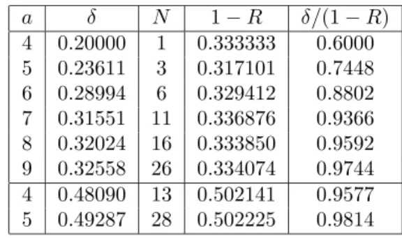
Table 1: Performance of some codes designed using the procedure described in Section 3.4. at rates close to 2/3 and 1/2. δ is the code threshold (maximum allowable value ofp),N the number of terms inλ(x), andRthe rate of the code.
a δ N 1−R δ/(1−R) 4 0.20000 1 0.333333 0.6000 5 0.23611 3 0.317101 0.7448 6 0.28994 6 0.329412 0.8802 7 0.31551 11 0.336876 0.9366 8 0.32024 16 0.333850 0.9592 9 0.32558 26 0.334074 0.9744 4 0.48090 13 0.502141 0.9577 5 0.49287 28 0.502225 0.9814
performed for systematic RA codes.
4.
IRA CODES ON THE AWGN
CHANNEL
In this section, we will consider the behavior of IRA codes on the AWGN channel. Here there are only two possible inputs, 0 and 1, but the output alphabet is the set of real numbers: if thex is the input, then the output is y = (−1)x+z, where z
is a mean zero, variance σ2 Gaussian random
vari-able. For a given noise variance σ2, our objective
will be to find a left degree sequenceλ(x) such that the ensemble message error probability approaches zero, while the rate is as large as possible. Unlike the BEC, where we deal only with probabilities, in the case of the AWGN we must deal with probability densities. This complicates the analysis, and forces us to resort to approximate design methods.
4.1.
Gaussian Approximation
Wiberg [9] has shown that the messages passed in iterative decoding on the AWGN channel can be well approximated by Gaussian random variables, pro-vided the messages are in log-likelihood ratio form. In [6], this approximation was used to design good LDPC codes for the AWGN channel.
In this subsection, we use this Gaussian approx-imation to design good IRA codes for the AWGN channel. Specifically, we approximate the messages from check nodes to variable nodes (both informa-tion and parity) as Gaussian at every iterainforma-tion. For a variable node, if all the incoming messages are sian, then all the outgoing messages are also Gaus-sian because of (4). A GausGaus-sian distributionf(x) is called consistent [5] iff(x) = f(−x)ex for ∀x ≤0.
The consistency condition implies that the mean and variance satisfyσ2= 2µ. For the sum-product
algo-rithm, it has been shown [2] that consistency is pre-served at message updates of both the variable and
check nodes. Thus if we assume Gaussian messages, and require consistency, we only need to keep track of the means. To this end, we define a consistent Gaussian densitywith meanµto be
Gµ(z) = 1 √ 4πµe −(z−µ)2/4µ . (27) The expected value of tanhz
2 for a consistent
Gaus-sian distributed random variable z with mean µ is then E[tanhz 2] = +∞ −∞ Gµ(z) tanh z 2dz =φ(µ). (28) It is easy to see that φ(u) is a monotonic increas-ing function of u; we denote its inverse function by
φ(−1)(y). Letµ(l)
L andµ
(l)
R be the means of the
mes-sage from check nodes to variable nodes on the left (i.e., information nodes) and on the right (i.e., par-ity nodes) at the lth iteration. We want to obtain expressions forµ(Ll+1) andµR(l+1)in terms ofµ(Ll)and
µ(Rl). A message from a degree-iinformation node to a check node at the lth iteration, is Gaussian with mean (i−1)µ(Ll)+µo, where µois the mean of
mes-sage mo in (4). Hence ifvL denotes the message on
a randomly selected edge from an information node to a check node, the density ofvL is
J
i=1
λiG(i−1)µ(l)
L +µo(z). (29)
From (29) and (28) we obtain:
E[tanhvL 2 ] = J i=1 λiφ((i−1)µL(l)+µo). (30)
Similarly, if vR denotes the message on a
ran-domly selected edge from a parity node to a check node, E[tanhvR 2 ] =φ(µ (l) R +µo). (31) Because of (5) we have E[tanhm(u→v) 2 ] = w=v E[tanhm(w→u) 2 ]. (32) Denote a message from a check node to an informa-tion node, resp. parity node, by uL, resp, uR.
Re-placing E[tanhm(w2→u)] with the right side of (30) or (31) depending upon whether the message comes from the left or right, (32) implies:
E[tanhuL 2 ] =E[tanh vL 2 ] a−1E[tanhvR 2 ] 2 = ( J i=1 λiφ((i−1)µ(Ll)+µo))a−1(φ(µ(Rl)+µo))2, E[tanhuR 2 ] =E[tanh vL 2 ] aE[tanhvR 2 ] = ( J i=1 λiφ((i−1)µ(Ll)+µo))aφ(µ(Rl)+µo).
Using the definition ofφ(µ) in (28), we thus have the following recursion forµ(Ll) andµ(Rl):
φ(µ(Ll+1)) = ( J i=1 λiφ((i−1)µ (l) L +µo))a−1× (φ(µ(Rl)+µo))2, (33) φ(µ(Rl+1)) = ( J i=1 λiφ((i−1)µL(l)+µo))a× φ(µ(Rl)+µo). (34)
In order to have arbitrary small bit error probabil-ity, the meansµ(Ll) andµ(Rl) should approach infinity as l approaches infinity. In the next subsection, we derive a sufficient condition for this.
4.2.
Fixed point analysis
We now assume that iterative dedoding has reached a fixed point of (33) and (34), i.e.,µ(Ll+1)=µ(Ll)=µL
andµ(Rl+1)=µ(Rl)=µR. Denote
J
i=1λiφ((i−1)µL+
µo) byx. From (30) we can see that 0< x <1 and
x→ 1 if and only if µL → ∞. From (34) it’s easy
to show that µR is a function of x, denoted by f,
i.e., µR =f(x). Then, dividing (33) by the square
of (34) gives us:
φ(µL) =φ2(µR)/xa+1=φ2(f(x))/xa+1. (35)
Now replacing µL with φ(−1)(φ2(f(x))/xa+1) into
the definition ofx, we obtain the following equation for the fixed pointx:
x= J i=1 λiφ(µo+ (i−1)φ(−1)( φ2(f(x)) xa+1 )). (36)
If this equation doesn’t have a solution in the in-terval [0,1], then the decoding bit error probability converges to zero. Therefore, if we have
F(x)= J i=1 λiφ(µo+ (i−1)φ(−1)( φ2(f(x)) xa+1 ))> x, (37) for anyx∈[x0,1), wherex0is the value ofxat the
first iteration, then (the Gaussian approximation to) iterative decoding is successful.
Since the rate of the code is given by (cf. (8)):
iλi/i
1/a+iλi/i
to maximize the rate, we should maximizeiλi/i.
Thus, under the Gaussian approximation, the prob-lem of finding a good degree sequence for IRA codes is converted to the following linear programming prob-lem:
Linear Programming Problem. Maximize J
i=1
λi/i, (39)
under the condition
F(x)> x, ∀x∈[x0,1]. (40)
We have designed some degree sequences for IRA codes using this linear programming methodology. The results are presented in Tables 2 (code rate ≈ 1/3) and 3 (code rate≈1/2). After using the heuris-tic Gaussian approximation method to design the de-gree sequences, we used exact density evolution to determine the actual noise threshold. (In every case, the true iterative decoding threshold was better than the one predicted by the Gaussian approximation.)
a 2 3 4 λ2 0.139025 0.078194 0.054485 λ3 0.222155 0.128085 0.104315 λ5 0.160813 λ6 0.638820 0.036178 0.126755 λ10 0.229816 λ11 0.016484 λ12 0.108828 λ13 0.487902 λ14 λ16 λ27 0.450302 λ28 0.017842 rate 0.333364 0.333223 0.333218 σGA 1.1840 1.2415 1.2615 σ∗ 1.1981 1.2607 1.2780 (Eb N0) ∗(dB) 0.190 -0.250 -0.371 S.L. (dB) -0.4953 -0.4958 -0.4958 Table 2: Good degree sequences yielding codes of rate approximately 1/3 for the AWGN channel and witha= 2,3,4. For each sequence the Gaussian ap-proximation noise threshold, the actual sum-product decoding threshold, and the corresponding (Eb
N0)
∗ in
dB are given. Also listed is the Shannon limit (S.L.)
For example, consider the “a= 3” column in Table 2. We adjust Gaussian approximation noise threshold
σGA to be 1.2415 to have the returned optimal
se-quence having rate 0.333223. Then applying the exact density evolution program on this code, we obtain the actual sum-product decoding threshold
σ∗= 1.2607, which corresponds toEb/N0=−0.250
dB. This should be compared to the Shannon limit for the ensemble of all linear codes of the same rate, which is −0.4958 dB. As we increase the parame-ter a, the ensemble improves. For a = 4, the best code we have found has iterative decoding threshold
Eb/N0 = −0.371 dB, which is only 0.12 dB above
the Shannon limit.
The above analysis is forbit error probability. In order to have zero worderror probability, it is nec-essary to haveλ2 = 0. (This can be proved by the
following argument: ifλ2>0, then in the ensemble,
asn→ ∞, the average number of weight 2 codewords is bounded away from zero. Hence even a maximum-likelihood decoder would have non-zero decoding er-ror probability.) In Table 3, we compare the noise thresholds of codes with and withoutλ2= 0.
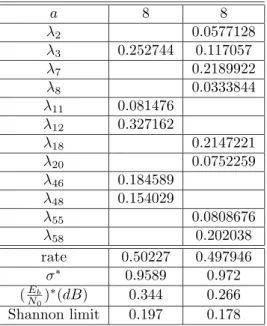
a 8 8 λ2 0.0577128 λ3 0.252744 0.117057 λ7 0.2189922 λ8 0.0333844 λ11 0.081476 λ12 0.327162 λ18 0.2147221 λ20 0.0752259 λ46 0.184589 λ48 0.154029 λ55 0.0808676 λ58 0.202038 rate 0.50227 0.497946 σ∗ 0.9589 0.972 (Eb N0) ∗(dB) 0.344 0.266 Shannon limit 0.197 0.178
Table 3: Two degree sequences yielding codes of rate≈ 1/2 with a = 8. For each sequence, the ac-tual sum-product decoding threshold, and the corre-sponding (Eb
N0)
∗ in dB are given. Also listed is the
Shannon limit.
We chose rate one-half because we wanted to com-pare our results with the best irregular LDPC codes obtained in [5]. Our best IRA code has threshold 0.266 dB, while the best rate one-half irregular LDPC code found in [5] has threshold 0.25 dB. These two codes have roughly the same decoding complexity, but unlike LDPC codes, IRA codes have a simple linear encoding algorithm.
4.3.
Simulation Results
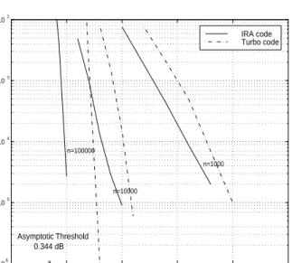
We simulated the rate one-half code with λ2 =
0 in Table 3. Figure 2 shows the performance of that particular code, with information block lengths 103, 104, and 105. For comparison, we also show the
performance of the best known rate 1/2 turbo code for the same block length.
0 0.5 1 1.5 2 2.5 106 105 104 103 102 SNR (dB) BER n=1000 n=10000 n=100000 IRA code Turbo code Asymptotic Threshold 0.344 dB
Figure 2: Comparison between turbo codes (dashed curves) and IRA codes (solid curves) of lengthsn= 103,104,105. All codes are of rate one-half.
5.
CONCLUSIONS
We have introduced a class of codes, the IRA codes, that combines many of the favorable attributes of turbo codes and LDPC codes. Like turbo codes (and unlike LDPC codes), they can be encoded in linear time. Like LDPC codes (and unlike turbo codes), they are amenable to an exact Richardson-Urbanke style analysis. In simulated performance they appear to be slightly superior to turbo codes of comparable complexity, and just as good as the best known irregular LDPC codes. In our opinion, the im-portant open problem is to prove (or disprove) that IRA codes can be decoded reliably in linear time at rates arbitrarily close to channel capacity. We know this to be true for the binary erasure channel, but for no other channel model. If this should turn out ot be true, we would argue that IRA codes definitively solve the problem posed implicitly by Shannon in 1948. If it is not true, then researchers should search for an even better class of code ensembles.
REFERENCES
[1] D. Divsalar, H. Jin, and R. J. McEliece, “Cod-ing theorems for ‘turbo-like’ codes,” pp. 201-210 in Proc. 36th Allerton Conf. on Communi-cation, Control, and Computing. (Allerton, Illi-nois, Sept. 1998).
[2] T. J. Richardson and R. Urbanke, “The capacity of low-density parity-check codes under message passing decoding,” submitted to IEEE Trans. Inform. Theory.
[3] M. Luby, M. Mitzenmacher, A. Shokrollahi, D. Spielman, and V. Stemann, “Practical loss-resilient codes,” Proc. 29th ACM Symp. on the Theory of Computing (1997), pp. 150-159. [4] M. Luby, M. Mitzenmacher, A. Shokrollahi, and
D. Spielman, “Analysis of low-density codes and improved designs using irregular graphs,” Proc. 30th ACM Symp. on the Theory of Computing (1998), pp. 249-258.
[5] T. J. Richardson, A. Shokrollahi,, and R. Ur-banke, “Design of provably good low-density parity-check codes,” submitted toIEEE Trans. Inform. Theory.
[6] S.-Y. Chung, R. Urbanke,, and T. J. Richard-son, “Analysis of sum-product decoding of low-density parity-check codes using a Gaussian ap-proximation,” submitted to IEEE Trans. In-form. Theory.
[7] D. Divsalar, S. Dolinar, and F. Pollara, “Itera-tive turbo decoder analysis based on Gaussian density evolution,” submitted to IEEE J. Se-lected Areas in Comm.
[8] M. A. Shokrollahi, “New sequences of linear time erasure codes approaching channel ca-pacity,” Proc. 1999 ISITA (Honolulu, Hawaii, November 1999) pp. 65–76.
[9] N. Wiberg, “Codes and decoding on general graphs,” dissertation no. 440, Link¨oping Studies in Science and Technology, Link¨oping, Sweden, 1996.
[10] J. Hagenauer, E. Offer, and L. Papke, “Itera-tive decoding of binary block and convolutional codes,” IEEE Trans. Inform. Theory, vol. IT-42, no. 2 (March 1996). pp. 429–445.