University of Windsor University of Windsor
Scholarship at UWindsor
Scholarship at UWindsor
Electronic Theses and Dissertations Theses, Dissertations, and Major Papers
2013
Estimating Deep Web Properties by Random Walk
Estimating Deep Web Properties by Random Walk
Sajib Kumer Sinha University of Windsor
Follow this and additional works at: https://scholar.uwindsor.ca/etd
Recommended Citation Recommended Citation
Sinha, Sajib Kumer, "Estimating Deep Web Properties by Random Walk" (2013). Electronic Theses and Dissertations. 4868.
https://scholar.uwindsor.ca/etd/4868
This online database contains the full-text of PhD dissertations and Masters’ theses of University of Windsor students from 1954 forward. These documents are made available for personal study and research purposes only, in accordance with the Canadian Copyright Act and the Creative Commons license—CC BY-NC-ND (Attribution, Non-Commercial, No Derivative Works). Under this license, works must always be attributed to the copyright holder (original author), cannot be used for any commercial purposes, and may not be altered. Any other use would require the permission of the copyright holder. Students may inquire about withdrawing their dissertation and/or thesis from this database. For additional inquiries, please contact the repository administrator via email
Estimating Deep Web Properties
by Random Walk
by
Sajib Kumer Sinha
A Thesis
Submitted to the Faculty of Graduate Studies
through Computer Science
in partial fulfilment of the requirements for
the Degree of Master of Science at the
University of Windsor
Windsor, Ontario, Canada 2013
c
Estimating Deep Web Properties by Random Walk
by
Sajib Kumer Sinha
APPROVED BY:
Dr. Yunbi An, External Reader Odette School of Business
Dr. Dan Wu, Internal Reader School of Computer Science
Dr. Jianguo Lu, Advisor School of Computer Science
Dr. Subir Bandyopadhyay, Chair of Defense School of Computer Science
Author’s Declaration of Originality
I hereby certify that I am the sole author of this thesis and that no part of this thesis has been published or submitted for publication.
I certify that, to the best of my knowledge, my thesis does not infringe upon anyone’s copyright nor violate any proprietary rights and that any ideas, tech-niques, quotations, or any other material from the work of other people included in my thesis, published or otherwise, are fully acknowledged in accordance with the standard referencing practices. Furthermore, to the extent that I have included copyrighted material that surpasses the bounds of fair dealing within the meaning of the Canada Copyright Act, I certify that I have obtained a written permission from the copyright owner(s) to include such material(s) in my thesis.
I declare that this is a true copy of my thesis, including any final revisions, as approved by my thesis committee and the Graduate Studies office, and that this thesis has not been submitted for a higher degree to any other University or Institution.
Abstract
The deep web is the part of World Wide Web that is hidden under form-like
inter-faces and can be accessed by queries only. Global properties of a deep web data
source such as average degree, population size need to be estimated because the
data in its entirety is not available. When a deep web data source is modelled
as a document-term bipartite graph, the estimation can be performed by random
walks on this graph. This thesis conducts comparative studies on various
ran-dom walk sampling methods, including Simple Ranran-dom Walk (SRW), Rejection
Random Walk (RRW), Metropolis-Hastings Random Walk (MHRW) and uniform
random sampling. Since random walks are conducted by queries in searchable
interfaces, our study has focused on the overall sampling cost and the estimator
performance in terms of bias, variance and RRMSE in this particular setting. From
our experiments performed on Newsgroup data we find that MHRW results higher
variance and RRMSE especially when the degree distribution follows the power
law. On the other hand RRW performs worse in terms of query cost as it rejects
too many samples. Compared to MHRW and RRW, SRW has low variance and
RRMSE. Besides, SRW outperforms the real uniform random samples when the
distribution follows the power law.
Dedication
To my mother Rina Sinha, father Ranada Prasad Sinha and my loving sister
Susmita Sinha for their unconditional love, support and endless encouragements.
Also to the workers of my motherland Bangladesh for their contribution to my
country...
Acknowledgements
Firstly, I would like to thank my parents. Without their encouragement, support
and love, it would not be possible for me to reach here.
I would like to express my deepest appreciation to my advisor, Dr. Jianguo
Lu, for his motivation, support and invaluable suggestions in guiding me towards
the successful completion of this research work. Without his generous funding
and advice, it would be hard for me to finish this research.
I would like to express my great gratitude to Dr. Yunbi An, Odette School of
Business, and Dr. Dan Wu, School of Computer Science for giving me corrections
and constructive criticism to improve the quality of this research, for their patience
in arranging the time of my proposal and defense, and for being in the committee,
and Dr. Subir Bandyopadhyay for serving as the chair of the committee.
I gratefully acknowledge the assistance of Md. Rajibul Mian, Gunjan Soni and
Numanul Subhani for their helpful discussion and support.
Finally, I want to extend my gratitude to my friends, the faculty members and
staff of the School of Computer Science for their friendly suggestions and support
during my study at University of Windsor.
Contents
Author’s Declaration of Originality iii
Abstract iv
Dedication v
Acknowledgements vi
List of Figures ix
List of Tables xi
List of algorithms xiii
1 Introduction 1
1.1 Deep Web . . . 1
1.2 Deep Web Sampling . . . 2
1.3 Thesis Problem and Contribution . . . 5
1.4 Thesis Organization. . . 6
2 Related Work 7
CONTENTS viii
2.1 Random Query based approaches . . . 7
2.2 Random Walk based approaches . . . 10
3 Estimation by Random Walk Sampling 13 3.1 Deep Web as Graph . . . 13
3.2 Random Walk on a Graph . . . 17
3.3 Simple Random Walk (SRW) sampling . . . 18
3.4 Rejection Random Walk (RRW) sampling . . . 21
3.5 Metropolis-Hastings Random Walk (MHRW) sampling . . . . 26
4 Experiments and Results 32 4.1 Data set . . . 33
4.2 Documents . . . 33
4.2.1 Sampling distribution. . . 34
4.2.2 Estimate average degree . . . 38
4.3 Terms . . . 50
4.3.1 Sampling distribution. . . 50
4.3.2 Estimate average degree . . . 53
5 Conclusions and Future Work 60
Bibliography 62
List of Figures
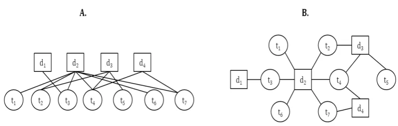
3.1 A) Deep web source as a bipartite graph B) same graph in spring
model . . . 14
3.2 An example of SRW sampling . . . 20
3.3 An example of RRW sampling . . . 25
3.4 Deep web source as a bipartite graph . . . 29
3.5 An example graph . . . 30
4.1 (A) Degree Distribution of whole Newsgroup data. (B) Only doc-ument degree distribution. (C) Only term degree distribution . . 34
4.2 Degree distribution of document samples of size 1000 using dif-ferent sampling methods from Newsgroup data. . . 36
4.3 CCDF of documentsamples of size 1000 using different sampling methods from Newsgroup data. . . 37
4.4 Box plots of estimated hdegi for documents using different sam-pling methods with different sample size and 200 iteration from Newsgroup data. . . 39
LIST OF FIGURES x
4.5 Bias, RSE and RRMSE of all documents average degree
esti-mation on newsgroup data over 200 runs using different sampling
methods.. . . 40
4.6 Box plots of estimated hdegi for documents using different
sam-pling methods with different cost and 200 iteration from
News-group data. . . 42
4.7 Bias, RSE and RRMSE of all documents average degree
esti-mation on newsgroup data over 200 runs using different sampling
methods with different cost. . . 43
4.8 Box plot of document-term sample ratio in different size of steps
by MHRW from Newsgroup data on 200 runs. . . 48
4.9 Degree distribution of term samples of size 1000 using different
sampling methods from Newsgroup data. . . 51
4.10 CCDF of termsamples of size 1000 using different sampling
meth-ods from Newsgroup data. . . 52
4.11 Box plots of estimated hdegi for terms using different sampling
methods with different sample size and 200 iteration from
News-group data. . . 53
4.12 Bias and RSE of alltermsaverage degree estimation on newsgroup
data over 200 runs using different sampling methods. . . 54
4.13 Box plots of estimated hdegi for terms using different sampling
methods with different cost and 200 iteration from Newsgroup data. 57
4.14 Bias, RSE and RRMSE of allterms average degree estimation on
newsgroup data over 200 runs using different sampling methods
List of Tables
4.1 Statistics of Newsgroup data . . . 33
4.2 Bias, RSE and RRMSE of all documents average degree
esti-mation on newsgroup data over 200 runs using different sampling
methods with different sample size. . . 41
4.3 Bias, RSE and RRMSE of all documents average degree
esti-mation on newsgroup data over 200 runs using different sampling
methods with different cost. . . 44
4.4 Ratio of the RSE of estimation in terms of valid sample size
(RSE-valid) and cost (RSE-cost) after 200 iteration using RRW . . . 45
4.5 Sample rejection rate rrsample for different iteration by RRW from
Newsgroup data . . . 46
4.6 Average Document-term sample ratio in different size of steps by
MHRW from Newsgroup data on 200 runs . . . 48
4.7 State rejection raterrsamplefrom different iteration by MHRW from
Newsgroup data . . . 49
LIST OF TABLES xii
4.8 Bias, RSE and RRMSE of allterms average degree estimation on
newsgroup data over 200 runs using different sampling methods
with different sample size. . . 56
4.9 Bias, RSE and RRMSE of allterms average degree estimation on
newsgroup data over 200 runs using different sampling methods
List of Algorithms
1 Simple Random Walk (SRW) sampling . . . 19
2 Rejection Random Walk (RRW) sampling . . . 23
3 Accept-RR. . . 24
4 Metropolis-Hastings Random Walk (MHRW) sampling . . . . 28
5 Accept-MH . . . 28
Chapter 1
Introduction
1.1
Deep Web
The deep web [9] is the part of WWW which have no specific hyper-links
to extract and are not indexable by the search engines. These are the pages
which are generated dynamically from the back-end data sources and can be
extracted only by its search interfaces. All dynamic pages behind the search
engines, content without in-links, limited access content, scripted content,
con-textual web are part of the deep web.For example, The Leddy Library site of
university of Windsor, Google’s index, The New York times site, all are part of
the deep web resources. Deep web properties estimation and evaluation such
as size, degree distribution, corpus freshness evaluation, spam evaluation,
se-curity evaluation and many more are buzzing issues for many researchers and
organizations [28]. Besides deep web properties are important parameters of
many more algorithms in distributed Information Retrieval system [12, 41].
In real application web marketing is a major concern for all business
CHAPTER 1. INTRODUCTION 2
zations and these kinds of deep web analysis can be more beneficial for those
marketing people to determine the importance and influence of a particular
web source in the real market. For example, size estimation can help to
de-termine which online library is rich with books, which social network covers
the maximum individuals, which search engine corpus is more updated and
content rich, which blogger is more influential upon the society.
When deep web is represented as a document-term graph, degree
distribu-tion, average degree, etc. are of great interest to the researchers to estimate
other properties such as population size. But calculating average degree is
not that straightforward as the deep web data in its entirety is not accessible
and much larger than the surface web. Besides, it is not efficient to crawl
and determine its different properties mentioned above as the size of the deep
web itself is an important parameter for the deep web crawler and extractor
[23, 34, 16]. Moreover, we have the issues of network bandwidth, we have
limited number of permitted queries over a search interface, limited number
of access from a certain IP and many more. As a result estimation is needed
to determine those properties. Hence, the sampling comes into consideration
which is very popular regarding this matter.
1.2
Deep Web Sampling
Sampling is a statistical technique in which a small part of large population
CHAPTER 1. INTRODUCTION 3
The selection of samples depends on the sampling design. There are lot of
sampling techniques in use for different estimation process in different areas.
As we have black box access to the deep web data [7] via its publicly available
search interface, query based sampling [13] is required.
Query based sampling was first proposed by Callan et al [13] for
acquir-ing resource description of databases. Resource description mainly consists
of vocabulary and frequency information [12]. In query based sampling a
query term needs to be submitted to the search interface and samples can be
obtained randomly from the matched documents. Here matched document
refers to the document which contains that submitted query term. Based on
the probability of a node to be sampled, sampling techniques can be
catego-rized into two different categories called Probability Proportion to Size (PPS)
and Uniform Random(UR) sampling.
In PPS sampling probability of being sampled is proportional to its size,
what means larger documents or more frequent terms are more likely to be
sampled. In contrast, for UR sampling each document will have the equal
probability to be sampled. In this research average degree of documentshdegdi
and terms hdegti will be estimated, which can be helpful to derive whole
population size and degree variance.
Assume we have N number of documents with their corresponding degree
degd
i where i ∈ {1,2,3... N}. In this case the average degree is
hdegdi= 1
N
N
X
i=1
degid (1.1)
One straightforward way of estimation is via Uniform Random (UR)
CHAPTER 1. INTRODUCTION 4
Hence the average of the total population can be estimated by the arithmetic
mean of the obtained samples, which can be called as sample mean estimator
[
hdegiSM. For n number of UR document samples {d1, d2, d3, ...dn} ∈ D with
corresponding degreedegd
i, the sample mean estimator will be
\
hdegdi SM =
1
n
n
X
i=1
degdi (1.2)
The < deg\d>
SM is unbiased if samples are truly uniform random. But using
simple query based sampling UR samples can not be obtained for the
hetero-geneity of the degree which rather gives PPS samples. To overcome the issue
of heterogeneity various Monte Carlo simulation methods such as rejection
sampling, Metropolis Hasting algorithm, importance sampling, maximum
de-gree method have been used in different areas including search engine index
[11, 7, 8], surface web [22], graphs [30], online social network [17, 37], real
social network [40, 44], etc. But these methods are not always efficient.
Be-cause, Rejection sampling results higher query cost as it rejects too many
samples. Also Metropolis Hasting algorithm gets stuck in a smaller portion
of a large graph as it remains in the same state because of rejection. Hence
biased samples come into consideration.
To estimate average degree from the biased PPS samples harmonic mean
es-timator is being used by many researchers in deep web properties estimation
[33], in social network analysis [18, 26, 32] and peer to peer network analysis
[38], which can be derived from Hansen-Hurwitz estimator [20]. This
har-monic estimator also has been used in sociology to estimate drug addicts [40].
corre-CHAPTER 1. INTRODUCTION 5
sponding degree degdi, the harmonic mean estimator will be
\
hdegdi H =n
" n X
i=1 1
degd i
#−1
(1.3)
As the simple query based sampling such as simple random walk does not
have any rejection procedure (rejection of sample or state) it can cover more
of the graph with less query cost.
1.3
Thesis Problem and Contribution
Several research have been performed to estimate deep web properties such
as average degree. But the question which techniques perform better for the
estimation remains unanswered. Besides there was no explicit empirical
stud-ies on the cost of those sampling techniques. In this research our problem can
be defined as
Given a deep web data source, how to estimate the average degree of the
documents and terms using UR and PPS sampling, and which method can be
considered as the better one?
To solve this problem, we have experimented and evaluated various
sam-pling techniques, including UR samsam-pling and biased PPS samsam-pling. We have
estimated the average degree of documents and terms using both sampling
methods. Given the limited access capabilities provided by deep web data
sources, UR samples are usually hard to obtain. For obtaining UR
sam-ples We have experimented with two UR sampling method called Rejection
Random Walk(RRW) and Metropolis Hasting Random Walk (MHRW) on
vari-CHAPTER 1. INTRODUCTION 6
ance in estimation compared to all other methods. Because, MHRW gets stuck
and covers a small part of the graph in each iteration. Hence estimation
be-comes biased based on that covered area. Also RRW waste too many samples
because of its acceptance rejection procedure. Since UR sampling is costly
and inefficient, we have also experimented with one PPS sampling method
called Simple Random Walk. We have found that biased SRW performs
bet-ter than the RRW and MHRW for both documents and bet-terms. For betbet-ter
comparison we obtain real UR samples directly from the index and estimate
the average degree as well. Here we observe that UR performs better, when
the distribution has less heterogeneity. For documents UR performs better as
the document degree distribution follow the log normal form and for terms
where the degree distribution follows power law SRW outperforms UR. We
have also explained the cost of both RRW and MHRW in terms of rejection
rate and found sample rejection rate is the average degree of the distribution
and state rejection rate of MHRW also dependent on the average degree.
1.4
Thesis Organization
The rest of the thesis is organized as following. Chapter 2 discussed about
some major related works that have been performed before. In Chapter 3
we have explained some useful terms which can be handy for our analysis
and discussed our all approaches with example. Chapter 4 consists of our
experiments and results. Lastly in Chapter 5 we have stated our concluding
Chapter 2
Related Work
Query based sampling for surfacing deep web properties has been studied since
the advent of the query based search interfaces. Different research works on
query based sampling have been performed with different types of data such
as search engines index [4, 2, 11, 7, 8] or relational database tables [14, 15]or
social networks [17, 24, 46]. All query based sampling approaches can be
divided into two parts called Random Query and Random Walk sampling.
2.1
Random Query based approaches
Random query is a lexicon based approach where query needs to be selected
randomly from the lexicon or collection of queries and submitted to the search
interface. After that, one random document is being selected as a sample from
the matched documents.
CHAPTER 2. RELATED WORK 8
Random Query based PPS sampling
Bharat and Broder [10] first realized the necessity of obtaining random pages
from a search engine’s index for calculating the relative size and overlapping
between two search engines. To solve this problem they first introduced the
lexicon based approach where conjunctive and disjunctive queries are being
generated randomly from the lexicon and run in the public interface of the
Search engine.
In the same year another influential research had been performed by Lawrence
and Giles [28] where they have estimated the size of search engines by random
query selected from user query logs. But both of these methods were biased
towards content rich highly ranked documents as both of these methods are
PPS sampling.
Callan and Connell [12] have proposed a query based sampling algorithm
for acquiring resource description of the relational databases based on the
concept of Bharat and Broder [10]. Here initially one query term is selected
at random and run on the database. Based on the returned top N number
of documents resource description is updated. This process run many times
based on different query terms until stop condition reached. This algorithm
also have the option of choosing number of query terms, how many documents
to examine per query and the stop condition of the sampling.
Bar-Yossef and Gurevich [6] first used importance sampling method with
PPS samples which is more similar to ours approach. The authors define two
new estimators called Accurate Estimator and Efficient Estimator to estimate
CHAPTER 2. RELATED WORK 9
sampling methods. The Accurate estimator uses approximate weights and it
requires sending some queries to a search engine and the Efficient
Estima-tor uses deterministic approximate weights and it does not need any query.
They use the Rao-Blackwell theorem with the importance sampling method
to reduce estimation variance.
Random Query based UR sampling
In 2006 Bar-Yossef and Gurevich [5] introduced the concept of the Query
pool and used one of the Monte Carlo simulation methods called Rejection
sampling with random query to obtain uniform random samples from the
search engine’s index. In their pool based approach they have applied rejection
sampling twice. First they applied rejection sampling to select a query from
the query pool which overcomes the ranking bias and again they applied
rejection sampling to select document from the matched documents which
overcomes the degree bias. Because of applying rejection procedure twice
their query cost is very large.
After that Broder et al. [11] used the Pool based concept of Bar-Yossef
and Gurevich [5] and introduced their new algorithm with new low variance
estimator where they have used the concept of traditional Peterson estimator
[1]. They have carefully crafted the importance sampling method with naive
estimator to reduce the bias. The authors propose two approaches based on
a basic low variance and unbiased estimator. Their first method requires a
uniform random sample from the underlying corpus and after getting the
CHAPTER 2. RELATED WORK 10
sampling they use the rejection sampling method. The second approach is
based on two query pools where both pools are uncorrelated with respect to
a set of query terms. Next, using these two query pools, the corpus size is
estimated using the low variance estimator that taken into account.
2.2
Random Walk based approaches
In a random walk we start with a seed node and in each step it moves to its
neighbour at random with equal probability. Note that here query is being
selected randomly from the current document of the walk instead of selecting
from a predefined lexicon. More detail about random walk will be explained
in Chapter 3.
Random Walk based PPS sampling
Henzinger et al have proposed Multi thread crawler to estimate various
prop-erties of web pages. They do not introduce any new method rather they give
some suggestion to improve sampling based on random walk. Instead of
us-ing normal crawler they suggest to use the Mercator, a multi threaded web
crawler. Here each thread will begin with randomly chosen starting point and
for random selection they suggest to make a random jump to the pages which
are visited by at least one thread instead of following the hyper links.
Following the idea of Henzinger et al [22], Bar-Yossef et al [4] introduce
the Web walker to approximate certain aggregate queries about web pages.
CHAPTER 2. RELATED WORK 11
performs a regular undirected random walk and picks pages randomly from
its traversed pages. Starting page of the Web Walker is an arbitrary page
from strongly connected component of the web. But as it is a PPS sampling
estimation is biased.
Rusmevichientong et al.[39] proposed two new algorithms based on
ap-proach of Henzinger et al [22] and Bar-Yossef et al. [4]. The first algorithm
called Directed-Sample works on the arbitrary directed graph and the other
one called Undirected-Sample works on the undirected graph with additional
knowledge about inbound links which requires access to the search engine.
Both of the algorithms based on weighted random-walk methodology.
Lu et al. [33] have used biased PPS samples obtained by SRW to discover
the average degree and population size of the deep web. They have also used
the harmonic mean estimator with the biased samples to estimate those
prop-erties and shown PPS can outperform real UR when the degree heterogeneity
is larger.
Random Walk based UR sampling
In 2006, Bar- Yossef and Gurevich [5] used one of the Monte Carlo simulation
methods called Metropolis Hastings algorithm in their random walk approach
to obtain uniform random samples from the search engine’s index. To
over-come the ranking bias they have used those queries which neither overflows
nor underflows. The detail of the Metropolis algorithm is explained in Chapter
3.
CHAPTER 2. RELATED WORK 12
samples from the social network Facebook. They also have used the
Re-Weighted random walk method, which is similar to our method. Here
sim-ple random walk bias is corrected by re-weighting of measured values using
Hansen-Hurwitz estimator [20].
A rejection sampling based random walk method have been proposed
by Dasgupta et al [14] to obtain uniform random sample from hidden web
databases. The authors propose a new algorithm called HIDDEN-DB-SAMPLER,
which is based on random walk over the query spaces provided by the public
user interface. Three new ideas proposed by the authors are early detection of
underflow and valid tuples, random reordering of attributes, boosting
accep-tance probability via a scaling factor. However, they proposed their method
for sampling from a database that is hidden behind a form, structured in a
particular way which cannot be compared with the deep web general search
interfaces.
In all of those approaches, cost of those sampling techniques is not being
studied rigorously. However, Bar- Yossef and Gurevich [7] have presented
the theoretical cost analysis in their subsequent work which is represented
in terms of upper bound and lower bound. Besides it is specific to their
experimental set-up and parameters such as query pool, query cardinality
ratios, etc. Hence, there is no specific empirical studies to analyse the cost
of these deep web sampling techniques , and the question, which sampling
Chapter 3
Estimation by Random Walk
Sampling
3.1
Deep Web as Graph
A Graph G is an ordered pair G = (V, E) consisting of a set of nodes or vertices (V) and a set of edges (E) which connects a pair of vertices, and
V ∩E = φ [3]. A vertex presents in an edge is called end vertex. Note that a vertex might be present in a graph but may not be in any edges. Degree
of a vertexx (degx) refers to the number of edges that connects x with other
vertices. An undirected graph is an unordered pair G = (V, E) where edges have no direction, means for any two nodesa andb, edges (a→b) = (b→a). In this research only undirected graph will be considered.
Surface web can be represented using a graph where each web page is a
vertex and each hyper link is an edge [25]. In contrast, deep web data source
can be represented as a document-term bipartite graph containing two
CHAPTER 3. ESTIMATION BY RANDOM WALK SAMPLING 14
joint sets of vertices where each edge connects two disjoint sets[36, 45, 47].
The graph G can be represented as G= (D, T, E) and D∩T = Ø, where D
is the set of documents,T is the set of terms andE is an edge betweenDand
T which represents the presence of a term in a document. The degree of each vertex is the number of its adjacent nodes. More precisely document degree
ofdi (degid) is the number of distinct terms that contained by the documentdi
and term degree ofti (degti) is the number of documents matched when term
ti is being submitted to the search interface.
Figure 3.1: A) Deep web source as a bipartite graph B) same graph in spring model
Example 1: Deep Web as bipartite graph A deep web source with 4
documents consisting 7 distinct terms has been depicted in Figure 3.1 where
D={d1, d2, d3, d4}andT ={t1, t2, ...t7}. An edge d1−t5 refers that the term
t5 presents in document d1. According to the Figure 3.1 degree of documents
degd
1 = 1 and deg2d= 6. Apparently, term degree deg1t = 1 and deg4t = 3. The graph depicted in Figure 3.1 can be represented with an adjacency
CHAPTER 3. ESTIMATION BY RANDOM WALK SAMPLING 15
a bipartite graph it is called the bi-adjacency matrix which is am×n boolean matrix, where m and n represent the number of vertices in two disjoint sets. Bi-adjacency matrix of Figure3.1 is as following.
0 0 1 0 0 0 0
1 1 1 1 0 1 1
0 1 0 1 1 0 0
0 0 0 1 0 0 1
|D| × |T|bi-adjacency matrix
A Markov chain is a sequence of nodes or states where the transition of
next step is independent of previous or current states. If the current state of
a Markov chain is ni, it will move to an another node nj with a transition
probability pij which is independent of other nodes[19].
A matrix that represents all transition probabilities is called transition matrix
(T) which can be denoted as T = (pij)∀i, j ∈V where
pij =
1
degi, if ij∈E 0, otherwise.
(3.1)
Transition matrix of Figure 3.1 will be as following.
0 0 1 0 0 0 0
1/6 1/6 1/6 1/6 0 1/6 1/6 0 1/3 0 1/3 1/3 0 0 0 0 0 1/2 0 0 1/2
CHAPTER 3. ESTIMATION BY RANDOM WALK SAMPLING 16
|D| × |T| transition matrix
A Markov chain is time reversible if the forward and backward edges
be-longs to same distribution, which means there is a probability distributionπ
such that π(i)pij = π(j)pji [19]. In terms of uniform distribution transition
probability will be equal and Markov chain will be time reversible.
Before proceeding to the Random Walk sampling, some basic definitions
and properties of statistics will be explained, which will be helpful for our
analysis.
Degree varianceσ2 is the measure of how far all the degrees are spread out from the meanµ, which can be defined as [42]
σ2 =hdeg2i − hdegi2 (3.2)
For our estimation variance can be defined as following
σ2 = 1
n
n
X
i=1
(h[degii−h\degi)2 (3.3)
Standard error (SE) is the square root of the variance which is as following.
SE= v u u t 1
n
n
X
i=1
(h[degii−h\degi)2 (3.4)
The coefficient of variationγ is the ratio of the standard deviation and the mean. Standard deviation is nothing but the square root of variance or the
SE. Theγ can be expressed as following
γ2 = σ 2
hdegi2 =
hdeg2i
hdegi2 −1 (3.5)
A graph is said to be regular when each vertex has equal degree and when
CHAPTER 3. ESTIMATION BY RANDOM WALK SAMPLING 17
Bias of an estimation ˆx is defined as
Bias(ˆx) = E(ˆx)−x (3.6)
HereEis the expectation ofx, which represents the mean of all possible values ofx. When the number of possible value is large it can be approximated using the sample mean. For example if we want to find the bias of estimated average
document degree (h\degdi), Bias will be as following.
Bias(hdegddi) = E(h\degdi)− hdegdi (3.7)
= 1
N
N
X
i=1
\
hdegd
ii − hdeg
di. (3.8)
For evaluation of our estimation we have also used the Relative Rooted
MSE (RRMSE) which can be defined as following.
RRM SE(h[degi) = 1
hdegi
v u u t 1
n
n
X
i=1
(h[degii− hdegi)2 (3.9)
RRMSE is nothing but the RMSE normalized by the mean and RMSE
can be derived from the bias and variance as following.
RM SE2 =Bias2+var (3.10)
3.2
Random Walk on a Graph
A random walk is a time reversible finite Markov chain [31] which proceeds by
stepping forward to a neighbouring node from a current node on a given graph.
After n number of successful steps it returns n number of samples which are elements of a Markov chain. A random walk on graph depicted in Figure 3.1
CHAPTER 3. ESTIMATION BY RANDOM WALK SAMPLING 18
changing of nodes in each steps depends on the mechanism of the random walk.
Three different random walk called Simple Random Walk(SRW), Rejection
Random Walk (RRW) and Metropolis-Hastings Random Walk (MH-RW) have
been explained in the next subsections.
3.3
Simple Random Walk (SRW) sampling
In a Random Walk process, for a given graph (G) and an initial node (n0), in each t+ 1th step one neighbouring node (n
t+1) of current node (nt) is being
selected with equal probability deg1
nt. A simple random walk on the document-term bipartite graph can be described as following. First, a valid document-term t0 is being selected from a lexicon as a seed query to initiate the random walk.
Note that a term is called valid if it is being matched with at least one
doc-ument while submitted to search interface. Next, one of the neighbouring
nodes of t0 will be selected randomly with equal probability 1/degit, which
will be a document di. After that another neighbour of document di will be
selected randomly with equal probability 1/degid. Thus these processes will
continue until n number of samples are being obtained. Note that, to obtain a neighbouring node of a term we need to submit that term in the search
in-terface and one matched document needs to be taken randomly. On the other
hand to obtain a neighbouring node of a document we need to download that
document and one term need to be selected randomly from that document.
Complete algorithm can be represented as Algorithm 1.
CHAPTER 3. ESTIMATION BY RANDOM WALK SAMPLING 19
Algorithm 1Simple Random Walk (SRW) sampling
Input : t0 = seed term, sample size n.
Output: Set of nnumber of document samplesDs and term samplesTs with
their corresponding degrees.
Ds =Ts = empty lists;
i= 1;
di = select one neighbouring node oft0 with equal probability;
while i ≤ n do
add di and its degree degid to Ds;
ti = select one neighbouring node ofdi with equal probability;
add ti and its degree degit to Ts;
di+1 = select one neighbouring node ofti with equal probability;
i+ +;
end
return Ds and Ts;
search interface and one document need to be downloaded to obtain each
sample. For selecting random document from the matched documents we
do not required downloading all matched documents. For simplicity we have
assumed all matched documents are being returned by the search interface.
So, using the search interface we can get all matched documents with their
URL. In our algorithm we store all matched documents ID in a list of length
m(number of matched documents) and next, we generate a random numberr
between 1 tom and get the ID ofr−th document from the list and download. In our algorithm one document can be visited multiple times. In other words
it is a sampling with replacement.
After obtaining samples by SRW we will estimate the average degree using
the harmonic mean estimator which has been defined in Equation 1.3. One
work through example of whole process is given below.
Example 2: SRW sampling and estimation
CHAPTER 3. ESTIMATION BY RANDOM WALK SAMPLING 20
a simple random walk sampling can be as following.
Figure 3.2: An example of SRW sampling
Input: graph depicted in Figure 3.1,t0 =t2 and n= 3
Process: This walk will starts with the seed node t2. Next, it will select and move to one of its neighbours with equal probability 1/degt2 = 1/2. Assume it selects and moves to d2. Hence,d2 will be added as a document sample. In the next step, walk will select and move to another neighbour ofd2 with equal probability 1/6. Assume it selects and moves to t3. Therefore, it will add t3 as a term sample. This process will continue until it obtains 3 samples. One
possible walk on the given graph is d2−t3 −d2 −t7 −d4 −t4 and has been shown in Figure3.2. The output of this algorithm can be as following format.
Output:
Ts ={(t3,2),(t7,2),(t4,3)}
Ds ={(d2,6),(d2,6),(d4,2)}
After obtaining Document and term samples, our next task is average
degree estimation using the harmonic mean estimator. If we consider the
document degree, the real average document degree of given graph will be
hdegdi= 1 + 6 + 3 + 2
CHAPTER 3. ESTIMATION BY RANDOM WALK SAMPLING 21
If we estimate hdegdi using sample mean which will be biased towards higher degree as following.
\
hdegdi SM =
6 + 6 + 2
3 = 4.66 (3.12)
Hence we will estimate the average degree using harmonic mean estimator
which basically reduce the bias of higher degree as following.
\
hdegdi H =
3 1 6 +
1 6 +
1 2
= 3.6 (3.13)
The advantage of the SRW sampling is all parts of the graph can be
tra-versed regardless of the graph properties such as γ or the graph shape. Be-cause, algorithm always selects and moves to one of the neighbours of current
node with equal probability. But, SRW is a PPS sampling.
3.4
Rejection Random Walk (RRW) sampling
RRW is a UR sampling procedure which applies the rejection sampling [43]
on random walk. Rejection sampling is the most classical and popular Monte
Carlo simulation methods which uses the acceptance-rejection procedure.
As-sume in a space u, π is the target distribution which is hard to be sampled directly andpis the trial distribution which is easy to be sampled. Note that a sample space refers to all possible outcomes of a random trial or experiment
and a probability distribution is a function that specifies the probability of
each of the possible outcomes of a random experiment [27]. In this case a
Monte Carlo simulation method is a procedure which takes sample from pin order to generate samples fromπ.
CHAPTER 3. ESTIMATION BY RANDOM WALK SAMPLING 22
procedure generate samples from the trial distribution p, such as document
d1, d2, d3...dn. In our case trial distribution is the degree distribution from
where we can easily obtain sample by submitting query. The two other
proce-dures are used to calculate the unnormalized forms of that particular sample
on the target distribution (ˆπ) and trial distribution (ˆp) respectively. An un-normalized form ˆp(x) or ˆπ(x) refers to the relative weight which reflects the probability of element x to be sampled from that particular distribution [7].
As π is considered as the uniform distribution, the relative weight will be uniform. Hence, for all x ∈ u straightforward unnormalized form of π is 1. On the other hand unnormalized form of p is nothing but the deg(x), as in degree distribution the sampling probability is proportional to its degree.
According to the rejection sampling procedure it will repeatedly generates
samples from the trial distributionpunless it is being accepted by the accep-tance functiona(x) as following.
a(x) = πˆ(x)
Cpˆ(x) (3.14)
HereC is a known envelope constant where ∀x∈supp(p), C ≥maxπˆpˆ((xx)) and
supp(p) = {x∈u|p(x)>0}. Note that for UR sampling C can be taken as 1 to satisfy the envelop condition.
Now for obtaining UR samples ˆπ(x) = 1, p(x) = deg(x) and C = 1, the acceptance function can be simplified as following.
a(x) = 1
degx
(3.15)
CHAPTER 3. ESTIMATION BY RANDOM WALK SAMPLING 23
this acceptance function which is inversely proportional to the degree, is
actu-ally reducing the acceptance probability of documents with higher degree and
increasing the acceptance probability of documents with lower degree.
Even-tually, rejection sampling uses the acceptance-rejection procedure to bridge
the gap betweenp andπ. The efficiency of this sampling method depends on the similarity betweenpandπ[7]. More similarity betweenpandπmakes less rejection. Also the gap between C and maxπˆpˆ((xx)) is crucial for the efficiency. A high value of C makes more rejection and very low value can violates the envelope property.
Algorithm 2Rejection Random Walk (RRW) sampling
Input : t0 = seed term, sample size n.
Output: Set of nnumber of document samplesDs and term samplesTs with
their corresponding degrees.
Ds =Ts = empty lists;
i= 1;
di = select one neighbouring node oft0 with equal probability;
while Ds.size < n OR Ts.size < n do
if Accept(di) then
add di and its degree degid toDs;
end
ti = select one neighbouring node ofdi with equal probability;
if Accept(ti) then
add ti and its degree degit to Ts;
end
di+1 = select one neighbouring node ofti with equal probability;
i+ +;
end
return Ds and Ts;
A rejection sampling based random walk named Rejection Random Walk
(RRW) sampling is given in Algorithm2. The basic procedure of RRW
CHAPTER 3. ESTIMATION BY RANDOM WALK SAMPLING 24
Algorithm 3Accept-RR
Input : di ORti
Output: true ORf alse
size = degree of the document (degid) OR term (degit);
r = one random number between 1 to size;
if r == 1 then
returntrue;
else
returnf alse;
end
selects and moves to its neighbour with equal probability. But unlike the
SRW sampling, it accepts a document or term with an acceptance
probabil-ity of deg1
i. Hence, documents or terms with higher degree are getting lower probability to be sampled by the acceptance function. Algorithm3is
simulat-ing that acceptance probability. To simulate the acceptance probability one
random number r is being generated between 1 to degi and if r comes up 1,
document or term is being accepted as a sample. To calculate the document
degree particular document needs to be downloaded and for the term degree
certain term need to be submitted to the search interface. Likewise SRW,
RRW is also a sampling with replacement. One work through example of the
whole RRW sampling is given below.
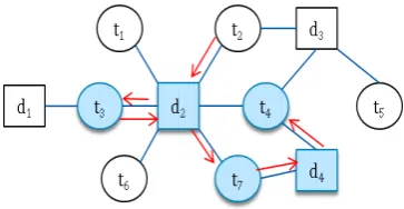
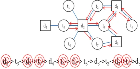
Example 3: RRW sampling and estimation
According to the graph depicted in Figure3.1 for a seed termt2 an output of a rejection random walk sampling can be as following.
Input: graph depicted in Figure 3.1, t0 =t2 and n = 3
Process: This walk will be initiated from the seed nodet2 and will select and move to one of its neighbours with equal probability 1/2. Assume it selects
CHAPTER 3. ESTIMATION BY RANDOM WALK SAMPLING 25
unless it passes the acceptance test with probability 1/deg2d. In the accep-tance test a random number r will be generated between 1 to degd2. assume
r = 3, so it is going to reject d2 as a sample and continue walk until it ac-cepts n number of samples. So, after t number of steps, algorithm might not accept t number of samples. One possible walk on the given graph can be
d2−t3−d2−t7−d4−t4−d3−t5−d3−t2−d2−t4−d3 and has been shown in Figure 3.3. Red sign is indicating the rejection on the same figure.
Figure 3.3: An example of RRW sampling
Finally, the output of this algorithm can be as following format.
Output:
Ts ={(t3,2),(t5,1),(t2,2)}
Ds ={(d4,2),(d3,3),(d3,3)}
RRW sampling is a UR sampling method. So, for average degree estimation
we can use the sample mean estimator as stated in Equation1.2. The average
document degree will be
\
hdegdi SM =
2 + 3 + 3
3 = 2.66 (3.16)
CHAPTER 3. ESTIMATION BY RANDOM WALK SAMPLING 26
restriction on the accepting of a sample. Hence RRW also able to traverse all
parts of the graph regardless of the graph properties such as γ or the graph shape. But, the problem of this algorithm is too many rejection.
Aftertnumber of iterations, if this algorithm accepts onlyanumber of samples we can define the sample rejection raterrsample as following
rrsample =
t−a
a (3.17)
For RRW sampling, sample rejection rate is proportional to the sampling cost.
In case of rejection it does not add that document or term as a sample. As
a result another iteration is needed to obtain another sample which increase
the query cost.
From the Figure3.3 it also can be observed that for obtaining 3 sample terms
and 3 documents algorithm rejected 4 documents and 3 terms. According to
this example for documents, samples rejection rate is following
rrsample =
7−3
3 = 1.33 (3.18)
From experiments conducted in this research we have found that
rrsanple=hdegi (3.19)
Detail of our experiments has been explained in Chapter 4.
3.5
Metropolis-Hastings Random Walk (MHRW)
sampling
Metropolis-Hastings algorithm is a Markov Chain Monte Carlo (MCMC)
dis-CHAPTER 3. ESTIMATION BY RANDOM WALK SAMPLING 27
tribution (p), to a new random walk that converges to a target distribution (π) [35, 21]. A MHRW sampler traverses on a Markov Chain to generate samples from a distribution by applying a acceptance-rejection procedure.
This acceptance-rejection procedure is being used to determine whether the
proposed state will be accepted as a next state of the random walk or not.
Eventually this acceptance-rejection procedure transforms the samples from
trial distribution (p) to target distribution (π). Note that this is different from the RRW sampling where we apply acceptance-rejection procedure during
ac-cepting a sample not in changing state.
The MH algorithm gives best output when the graph is ergodic and supp(p) = supp(π). Note that a graph is called ergodic when it is irreducible or strongly connected and aperiodic. The acceptance function of the MH algorithm is as
following.
aM H(x, y) =min{
π(y)P(y→x)
π(x)P(x→y),1} (3.20) Here,π(x) is the probability ofxto be chosen as a sample from the distribution
πandP(x→y) is the transition matrix which can be represented as following.
P(x→y) = 1
degx
(3.21)
Hence, after simplification acceptance function will be as following
aM H(x, y) = min{
degx
degy
,1} (3.22)
A Metropolis-Hastings algorithm based random walk is given in Algorithm
4. The foundation of this algorithm is also similar to SRW. But, MHRW
dif-fers from the SRW and RRW in state transition. In MHRW, algorithm selects
CHAPTER 3. ESTIMATION BY RANDOM WALK SAMPLING 28
Algorithm 4Metropolis-Hastings Random Walk (MHRW) sampling
Input : t0 = seed term, sample size n
Output: Set of nnumber of document samplesDs and term samplesTs with
their corresponding degrees.
Ds =Ts = empty lists;
current = select one neighbouring node oft0 with equal probability;
while Ds.size < n OR Ts.size < n do
next = select one neighbouring node ofcurrent with equal probability;
if Accept(current, next)then
current=next;
end
add current and its degree degcurrent toDs OR Ts;
end
return Ds and Ts;
Algorithm 5Accept-MH
Input : Two document or term nodes
Output: true ORf alse size1 = degree of current;
size2 = degree of next;
r = one random number between 1 to size2;
if r <=size1 then returntrue;
else
returnf alse;
end
it does not move to that neighbour unless it passes the acceptance test stated
earlier. Our Algorithm5is simulating the acceptance probability of Equation
3.22. If it passes the test it moves and add that particular neighbour as a
sample. Otherwise, it will remain in the same state and will add that current
node as a sample. One work through example of whole MHRW for document
sampling is given below.
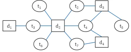
CHAPTER 3. ESTIMATION BY RANDOM WALK SAMPLING 29
Figure 3.4: Deep web source as a bipartite graph
Given the graph depicted in Figure 3.4 one possible MHRW sampling can be
as following
Input: graph depicted in Figure 3.4, t0 =t2 and n = 3
Process: Likewise other two random walks it will start with the seed node
t2 and select one of its neighbours, assume d2 with equal probability. But it will not move to d2 unless it passes the acceptance test with probability
min{1,degt2
degd
2
}. To simulate this probability a random number r will be
gener-ated from 1 to degd
2. If r < degt2 it will move to d2 and add d2 as a sample. Otherwise, it will remain in t2 and add t2 as a sample. Assume generated
r= 3, so it will not accept that state and will remain and addt2 as a sample. This process will continue until 3 document and term samples are being
ob-tained. Note that in MHRW afternnumber of iterationsnnumber of samples will be obtained regardless of the number of rejection. One possible walk can
bet2(seed)−t2−d3−t5−t5−d3−t4−d4. In this walk consecutive repetition of nodes means rejection of state. Finally, the output of this algorithm can
be as following format.
Output:
Ds ={(d3,3),(d3,3),(d4,2)}
CHAPTER 3. ESTIMATION BY RANDOM WALK SAMPLING 30
As MHRW produces UR sample, we will use the sample mean estimator stated
in Equation 1.2 to estimate the average degree. For our considered example
average document degree will be as following
\
hdegdi SM =
3 + 3 + 2
3 = 2.66 (3.23)
In MHRW whether it accepts or rejects, in each step algorithm will obtain
one sample. Therefore according to Equation 3.17 the rejection rate rr = 0 which is true in terms of sample acceptance. But, does this rejection of states
effects the process? if yes then how?
We have tried to explain this answer using another term named state rejection
rate. Forn number of iterations, if the algorithm accepts a0 number of states, we define the state rejection raterrstate as following
rrstate =
n−a0
a0 (3.24)
Though, rrstate does not effect the query cost but it can effects the sampling
Figure 3.5: An example graph
accuracy. For example let us consider the graph in Figure 3.5 where each
node has been labelled with their corresponding degree and cloud represents
sub-graph of the whole graph, if we applies MHRW with starting node 1 it
CHAPTER 3. ESTIMATION BY RANDOM WALK SAMPLING 31
1/1000 which is very low. Hence, even after 500 iterations current state might
be the node 1 and all obtained samples during this 500 iterations will be node
1, which might cause a great bias during estimation. So, higher state rejection
rate increase the cover time which means expected number of steps to reach
every node [31]. As a result the distinct number of nodes traversed by the
walk will be small.
In the example walk for obtaining 3 documents samples we need to make 5
iterations. Where the state rejection rate is
rrstate =
5−3
Chapter 4
Experiments and Results
In our estimation process for obtaining UR and PPS samples, our experiment
differs from query-based sampling [13] in the following aspects:
• All matched documents or terms are being returned as a query result
which means the ranking over the documents is ignored. Hence no query
overflow.
• All documents have been indexed with full length. That means no
trun-cation of document size.
• Duplicate and near-duplicate are not in consideration. That means
du-plicate and near dudu-plicate documents also have the equal probability to
be captured.
CHAPTER 4. EXPERIMENTS AND RESULTS 33
4.1
Data set
We use 20k Newsgroup data corpus consisting 19,996 xml documents including
some empty documents which have been excluded from our experiment, In
our experiments we have considered all single alphabetical words as our query
term and those are case insensitive. A statistical summary of the data set
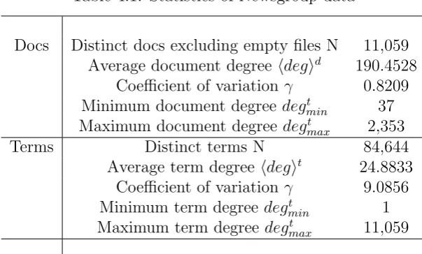
been given in Table 4.1.
Table 4.1: Statistics of Newsgroup data
Docs Distinct docs excluding empty files N 11,059 Average document degree hdegid 190.4528
Coefficient of variationγ 0.8209 Minimum document degree degt
min 37
Maximum document degreedegt
max 2,353
Terms Distinct terms N 84,644
Average term degreehdegit 24.8833
Coefficient of variationγ 9.0856 Minimum term degreedegt
min 1
Maximum term degree degt
max 11,059
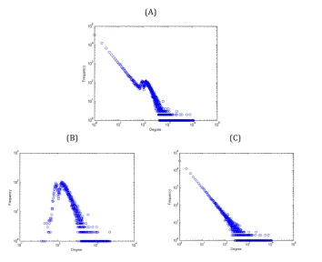
The degree distribution of newsgroup document-term graph is depicted
in Figure 4.1. Here we plot the frequency against degree. We can observe
that document degrees follow log-normal distribution whereas term degree
distribution follows the power law.
4.2
Documents
This section focuses on the estimation for documents. We report the
CHAPTER 4. EXPERIMENTS AND RESULTS 34
Figure 4.1: (A) Degree Distribution of whole Newsgroup data. (B) Only document degree distribution. (C) Only term degree distribution
methods.
4.2.1
Sampling distribution
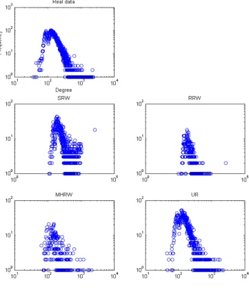
We compare the sample distributions that are obtained from four sampling
methods including SRW, RRW, MHRW and UR. We obtain 1000 samples and
depict in Figure4.2which is the the frequency-degree plot. From Figure4.2it
is observed that SRW sample distribution is different from the real documents
distribution. For SRW the tail part is higher compared to the real
distribu-tion, which proves that documents with higher degree have higher frequency
CHAPTER 4. EXPERIMENTS AND RESULTS 35
random samples which resemble the real distribution that is log-normal. But,
in frequency-degree plot RRW, MHRW and UR seems different because of
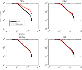
small sample size. For better observation we depict the corresponding CCDF
(Complementary Cumulative Distribution Function) in Figure4.3. For SRW,
CCDF line of sampled data goes upper than the real data as degree increases
which means documents with higher degree sample more. In contrast RRW,
MHRW and UR samples fits with the real data distribution as those are
CHAPTER 4. EXPERIMENTS AND RESULTS 36
CHAPTER 4. EXPERIMENTS AND RESULTS 37
CHAPTER 4. EXPERIMENTS AND RESULTS 38
4.2.2
Estimate average degree
Comparison in terms of valid sample size
In this section we compare the sampling methods with valid samples only,
disregard of the rejected samples during the sampling process. We show that
some sampling methods, for instance MHRW, is worse than UR even when
only valid samples are considered. Next section we will conduct the
compar-ison based on the actual sampling cost when the rejected samples are also
included as sample size.
After obtaining document samples by SRW, RRW, MHRW and real UR
sampling, we estimate the average degree of documents using harmonic mean
(for SRW) and sample mean (for RRW, MHRW, and UR) estimator stated
in Equations1.3 and1.2 respectively. We compare these four sampling
meth-ods for the estimation of the average degree of documents. Even though UR,
RRW, and MHRW all produce uniform random samples in theory, the
per-formances are different because RRW and MHRW obtain uniform random
samples only asymptotically.
First we give the box plots for the intuitive understanding of the
estima-tions. In Figure 4.4, for each sampling method we produce 10 box plots for
the sample sizes ranging between 1,000 and 10,000. Each box plot is obtained
from 200 runs. It shows that MHRW and RRW samplings results in larger
variations of the estimations.
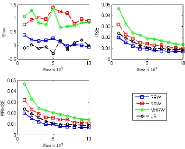
Next, we calculate the bias, relative standard error (RSE) and RRMSE of
respec-CHAPTER 4. EXPERIMENTS AND RESULTS 39
Figure 4.4: Box plots of estimatedhdegifordocuments using different sam-pling methods with different sample size and 200 iteration from Newsgroup data.
tively. RSE is the SE normalized by mean. Here bias evaluates how far the
estimation from the real value and RSE determines the variation of
estima-tions. The RRMSE helps us to evaluate the estimation based on both bias
and variance together.
In Table 4.2 we reported the bias, RSE and RRMSE of estimation using
different sampling methods for documents with different sample size. We also
plot these values in Figure 4.5, which gives a more detailed comparison in
terms of bias, rse, and rrmse.
First, we notice that UR does not show obvious bias as expected. Other
CHAPTER 4. EXPERIMENTS AND RESULTS 40
Figure 4.5: Bias, RSE and RRMSE of alldocuments average degree estima-tion on newsgroup data over 200 runs using different sampling methods.
walk mixing time. The samples are not strictly uniformly at random before
random walk mixing. The rse of the four sampling methods are also different.
SRW has the smallest variance while MHRW is the worst, because in different
iteration MHRW covers a certain part of the graph and reflects in estimation.
Figure4.5 also shows that the variance dominates the performance of the
estimators within this sample size range. Because the bias is rather small
CHAPTER 4. EXPERIMENTS AND RESULTS 42
Comparison in terms of cost
In previous experiments we estimate hdegi using valid samples excluding all rejected ones. In this section we conduct similar experiments considering cost.
In Figure 4.6 we depict the box plots of all estimations for documents using
different sampling methods over 200 runs considering cost or number of steps.
Figure 4.6: Box plots of estimatedhdegifordocuments using different sam-pling methods with different cost and 200 iteration from Newsgroup data.
From the boxplots in Figure4.6we observe that SRW and UR are the same
as before, since they do not incur extra costs. In SRW, each next random node
is taken as a valid sample and in UR sampling, we assume that random nodes
can be obtained directly.
In Table 4.3 we report the bias, RSE and RRMSE of estimation using
CHAPTER 4. EXPERIMENTS AND RESULTS 43
values in Figure 4.7.
CHAPTER 4. EXPERIMENTS AND RESULTS 45
For RRW, there are nodes that are accessed but not counted as valid
samples. In average RRW rejects hdegi number of samples but keeps only one of them as valid. Hence it estimateshdegi based on very small number of accepted samples compared to other methods and performs worst. Note that
if the real data variance is σ2, The relation between sample size n and SE is as following.
SE = √σ
n (4.1)
This means more samples result less SE. Ifn1 is the number of valid samples andn2is the cost including rejected samples wheren1 > n2. The ratio between two RSE will be
√ n1
√
n1/hdegi
=phdegi. Hence for documents RSE of estimation in terms of valid sample will be √190.45 = 13.80 times better than RSE of estimation in terms of cost. In Table 4.4 we report the ratio of both RSE
for RRW. We find the average ratio is 17.70 which is higher than 13.80. This
might happen because of less number of iterations.
Table 4.4: Ratio of the RSE of estimation in terms of valid sample size (RSE-valid)and cost (RSE-cost)after 200 iteration using RRW
Size×103 RSE-valid RSE-cost Ratio 1 0.463 0.0316 14.639 2 0.366 0.0224 16.343 3 0.332 0.0187 17.775
4 0.240 0.015 16.006
CHAPTER 4. EXPERIMENTS AND RESULTS 46
We experimented on sample rejection rate for RRW according to the
equa-tion3.17. We calculate the rejection rate to obtain different size of documents
and terms samples together. In Table4.5 we report the sample rejection rate
for both documents and terms from newsgroup data using RRW.
Table 4.5: Sample rejection raterrsample for different iteration by RRW from
Newsgroup data
T otalAccepted Documents Terms
×103 Accepted Rejected rr
sample Accepted Rejected rrsample
1 123 20963 170.43 877 19982 22.78
2 215 42982 199.92 1785 40945 22.94
3 350 66168 189.05 2650 63191 23.85
4 470 88134 187.52 3530 84101 23.82
5 558 109056 195.44 4442 104041 23.42
6 678 132982 196.14 5322 126951 23.85
7 821 153951 187.52 6179 146938 23.78
8 884 173851 196.66 7116 165764 23.29
9 1055 197818 187.51 7945 188763 23.76 10 1150 217803 189.39 8850 207706 23.47 Average 189.96 Average 23.50
From this table it can be observed that documents sample rejects more
than the terms sample. For documents, average sample rejection rate is 189.96
and document average degree is 190.4528. Like wise for terms average sample
rejection rate is 23.50 and term average degree is 24.8833. Hence we can infer
that sample rejection rate for RRW is equal to average degree.
This relation also can be derived as following. Assume, after N number of steps we obtainN number of samples with following degree
CHAPTER 4. EXPERIMENTS AND RESULTS 47
After rejection procedure we will have only n valid samples as following
1
dx1,
1
dx2,
1
dx3, ...
1
dxn
As those samples are uniform random the average of these samples will be
same as the real average degree.
1
n
Pn
i=1 1
degxi = 1
hdegi
Therefore,Pn
i=1 1
degxi =
n hdegi
Hence, for hdegni number of samples it will reject n. So, for 1 sample it rejects
hdegi. Hence the sample rejection rate is hdegi.
We also can observe that MHRW considering cost performs worse than
MHRW without cost. The reason is MHRW without cost consider larger
sample size than with cost and more samples reduce the RSE and RRMSE.
Note that cost 1000 does not provide equal number of documents or terms.
There is always a ratio between documents and terms samples. In our
ex-periment term nodes sample almost seven times more than document nodes.
Hence estimation perform based on less sample. Therefore, documents
sam-pling with fixed size performs better than documents samsam-pling with cost. We
also observe the ratio of obtained documents and terms sample by MHRW
in fixed number of cost. In Table 4.6 we report document-term sample ratio
in different size of steps. We also depicted the box plots of ratio in Figure
4.8. We can observe that the ratio is almost 0.13 which is the ratio between
documents and terms average degree 24.88/190.45 = 0.13.
We also calculate the state rejection rate of MHRW according to the
CHAPTER 4. EXPERIMENTS AND RESULTS 48
Table 4.6: Average Document-term sample ratio in different size of steps by MHRW from Newsgroup data on 200 runs
Cost×103 Average Doc/Term ratio
1 0.1538
2 0.1458
3 0.151
4 0.1443
5 0.1339
6 0.1394
7 0.1375
8 0.138
9 0.1341
10 0.1368
Figure 4.8: Box plot of document-term sample ratio in different size of steps by MHRW from Newsgroup data on 200 runs.
documents and terms using MHRW with different sample size from newsgroup
data.
From this table it can be observed that from a term node it rejects more
than from a document nodes. Which means it gets stuck more times in a term
node compared to a document node. For documents, average state rejection
CHAPTER 4. EXPERIMENTS AND RESULTS 49
Table 4.7: State rejection raterrsample from different iteration by MHRW from
Newsgroup data
Accepted From documents From terms
×103 Rejected rrstate Rejected rrstate
1 1228 1.228 14098 14.098 2 2377 1.1885 34133 17.0665 3 3737 1.2456 45023 15.0076 4 5013 1.2532 60668 15.167 5 5984 1.1968 72452 14.4904 6 7339 1.2231 83908 13.9846 7 8969 1.2812 102558 14.6511 8 9728 1.216 112099 14.0123 9 11211 1.2456 146384 16.2648 10 12106 1.2106 187450 18.745
CHAPTER 4. EXPERIMENTS AND RESULTS 50
4.3
Terms
This section focuses on the sampling and estimation for terms using all four
sampling methods.
4.3.1
Sampling distribution
We also compare terms sample distributions that are obtained from four
sam-pling methods. We obtain 1000 term samples and depict in Figure4.9 which
is the the frequency-degree plot. From Figure 4.9 it is observed that SRW
sample distribution is completely different from the real terms distribution.
For SRW the tail part is higher compared to the real distribution, which
proves that terms with higher degree have higher frequency in the sampled
data. Whereas RRW, MHRW and UR samples resemble the real distribution.
For better observation we also depict the corresponding CCDF in Figure4.10.
For SRW, CCDF line of sampled data goes upper than the real data as
de-gree increases which means terms with higher dede-gree sample more. Unlikely
RRW, MHRW and UR samples fits with the real data distribution as those
CHAPTER 4. EXPERIMENTS AND RESULTS 51
CHAPTER 4. EXPERIMENTS AND RESULTS 52