R E S E A R C H
Open Access
Long-term behavior of non-ferrous metal
price models with jumps
Jun Peng
1,2,3*and Jianbai Huang
1,3*Correspondence: [email protected] 1Business School, Central South University, Changsha, Hunan 410083, China
2School of Mathematics and Statistics, Central South University, Changsha, Hunan 410083, China Full list of author information is available at the end of the article
Abstract
In this paper, we study the long-term behavior of a class of stochastic non-ferrous metal prices with jumps. Suppose thatX(t) is a stochastic model for some metal price with Poisson jumps. For a suitable
μ
≥1, we prove thatt–μ0tX(s)dsconverges almost surely ast→ ∞. Finally, the model is applied to forecast the behavior of a two-factor affine model.MSC: 60H15; 86A05; 34D35
Keywords: long-term behavior; jump; geometric Brownian motion; convergence
1 Introduction
Non-ferrous metal resources commodity producers, consumers and investors face prob-lems resulting from the great variability in metal prices over time. The metal price fluctu-ations affect metal consumers by increasing or decreasing production cost. Obviously, the consumer wants the price to be as low as possible. Therefore, the metal price should not be too high to lose the clients because of the drastic competition arising from the open market. On the other hand, if the price is lower than the estimated random price in or-der to cover expenses and to hold some reserves, the companies would go bankrupt. In this light, it is very useful to study and to model the long-time behavior in a mathematical way. As discussed by Ahrens and Sharma [] (elsewhere [–]), natural resources com-modity prices exhibit stochastic trends. In order to capture the properties of empirical data, Brennan and Schwartz [] proposed a geometric Brownian motion (GBM) model for forecasting natural resources commodity pricesYt:
dYt=θYtdt+σYtdWt, t≥, y= ,
wheredWt is the increment in a Gauss-Wiener process with driftθ and instantaneous
standard deviationσ. A geometric Brownian motion or exponential Brownian motion is a continuous-time stochastic process in which the logarithm of the randomly varying quantity follows a Brownian motion or a Wiener process. It is applicable to mathematical modeling of some phenomena in financial markets. GBM is used as a mathematical model in financial markets and in forecasting prices. The GBM formula means that ‘in any in-terval of time, prices will never be negative and can either go up or down randomly as a function of their volatility’.
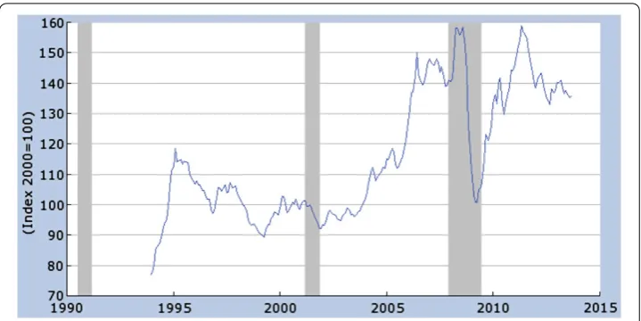
Figure 1 Monthly data for the price of aluminum and articles thereof (IP76) from January 1994 to October 2013.Shaded areas indicate US recessions. We quoted the data from US Department of Labor: Bureau of Labor Statistics.
One generalization of the GBM model is to use regime switching such as in [, ], to name a few. Hamilton [] characterizes business cycles as periods of discrete regime shifts, i.e., recessions are characterized belonging to one regime and expansions to another in a Markov-switching process. The main advantage of the Markov-switching space state model over the standard GARCH model is that in the case of the latter the unconditional variance is constant, while in the former the variance changes according to the state of the economy. However, the Markov-switching model has been criticized because it lacks transparency, is less robust and is difficult to apply [].
On the other hand, various economic shocks, news announcement, government policy changes, market demands may affect the metal price in a sudden way and generate non-ferrous metal price jumps. As indicated in Figure , the jumps do exist in the aluminum prices realization. This paper introduces a new comprehensive version of the long-term trend reverting jump and diffusion model. The behavior of historical non-ferrous metal prices includes three different components: long-term reversion, diffusion and jump. The long-term behavior of stochastic interest rate models was discussed in [–], where they studied the Cox-Ingersoll-Ross model.
In this paper, in order to incorporate sudden jumps in spot market, we consider the stochastic metal price model with jumps in the form
dX(t) =βX(t) +δ(t)dt+σX(t)dW(t) +
U
gX(t–),uN˜(dt,du), ()
whereX(t–) :=lims→tX(s). The integral
Ug(X(t–),u)N˜(dt,du) depends on the Poisson
measure and is regarded as a jump. Precise assumptions on the data of Equation () are given in Section .
2 The long-term behavior of stochastic metal price models with jumps
Let (,Ft,P) be a complete probability space in which two mutually independent
pro-cesses are defined: (Wt)t≥a standardd-dimensional Brownian motion andNa Poisson random measure on (, +∞)×(Z\ {}), whereZ⊂Rdis equipped with its Borel fieldB
Z,
with the Levy compensatorN˜(dt,dz) =dtν(dz),i.e.,{ ˜N((,t]×A) = (N–N˜)((,t]×A)}t> is anFtmartingale for eachA∈BZ. Henceν(dz) is a Poissonσ-finite measure satisfying
Zν(dz) <∞. We assume that there exist a sufficiently large constantγ > and a function
ρ:Rk→R+with
Zρ(z)ν(dz) <∞such that
b(t,x) –bt,x,x–x≤γx–x,
σ(t,x) –σt.x≤γx–x,
b(t,x)+σ(t,x)≤γ +|x|,
g(x,z) –gx,z≤Kx–x,
g(x,z)≤ρ(z) +|x|,
where ·,·and| · |denote the Euclidean scalar product and the norm, respectively. Obvi-ously, under the above assumptions, there exists a unique strong solution to () (see,e.g., []).
Lemma If X(t)satisfies()and P(X()≥) = ,then P(X(t)≥for all t≥) = .
Proof Leta= andak=exp(–k(k+ )/) fork≥, so that
ak–
ak
du
u =k. For eachk≥,
there clearly exists a continuous functionψk(u) with support in (ak,ak–) such that
≤ψk(u)≤
ku forak<u<ak–
andak–
ak ψk(u)du= . Defineϕk(x) = forx≥ and
ϕk(x) =
–x
dy
y
ψk(u)du forx< .
It is easy to observe thatϕ∈C(R,R) and –≤ϕk(x)≤ ifx< –akor otherwiseϕk(x) = ;
ϕ(x)≤kx if –ak–<x< –akor otherwiseϕ(x) = .
Moreover,
x––ak–≤ϕk(x)≤x– for allx∈R,
wherex–= –xifx< or otherwisex–= . For anyt≥, by Ito’s formula, we can derive
Eϕk
X(t)=Eϕk(X) +E
t
ϕkX(s) βX(s) +δ(s)ds
+σ
E
t
+E
Combining with the Gronwall inequality, we have
EX–(t) –ak–≤Eϕk
Proof By Ito’s formula, we have
de–kβtX(t)=e–kβt
Integrating from toτ and taking expectations on both sides, we have
Ee–kβτX(τ)≤C+
Theorem Let X(t)be a solution to()and assume that there isμ≥and a nonnegative random variableδ¯such that
lim
Then the following convergence holds:
Proof We use Kronecker’s lemma in [].
Dividing equation () byβ( +t)μgives the equality constantKdepending onω. A straightforward calculation shows that
∞
u+ dBuis a local martingale, it suffices to remark that
t
XuTn
u+ dBuis anLbounded martingale,
In order to evaluate the integral, we remark that
EXTn
In Lemma , we have obtained the inequality
Ee–kβτX(τ)≤C+CE
τ
Consequently,
Using this result, we obtain
t
Obviously, the first term is uniformly bounded in t. For the second term, we apply Fubini’s theorem to find a bound which does not depend ont,
t
The third term converges to by observing that
E
3 The long-time behavior of affine models
As an application of Theorem , we consider the long-time behavior of an affine model in a two-dimensional case,
usual hypothesis. Suppose that on this probability space the following objects are defined:
(ii) N(dt,du),N(dt,du)represent Poisson counting measures with characteristic measuresν(·)andν(·), respectively.
For model (), we are interested in the almost sure convergence of the long-term behav-iort–μt
Y(s)dsfor someμ≥.
The processY(t) has a reversion level X(t) which is a stochastic process itself. From Dawson and Li [], the equation system has a unique strong solution (X(·),Y(·)). More-over, (X(·),Y(·)) is an affine Markov process. Now, we give the main theorem of this sec-tion.
Theorem Assume that(X(·),Y(·))is a solution to the equation system().Then we have
tμ
t
Y(s)ds→– δ¯
ββ
a.s. as t→ ∞.
Proof It can be obtained by similar arguments as Theorem .
Another application of Theorem is that if the average of the drift converges almost surely to a constant, then the long-term trend of the model will revert to a line almost surely.
Corollary Letδ:ω×R+→R+and there exist constantsμ≥andδ¯≥such that
lim
t→∞
tμ
t
δ(s)ds→ ¯δ a.s.
Then the following convergence holds for equation():
tμ
t
X(s)ds→–δ¯
β a.s. as t→ ∞.
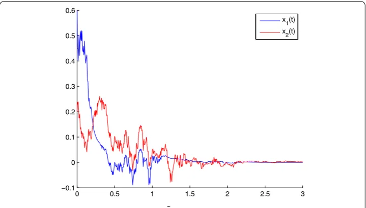
In Figure , the long-term behavior of the model is plotted withμ=β=σ= andδ¯= .
Competing interests
The authors declare that they have no competing interests.
Authors’ contributions
All authors completed the paper together. All authors read and approved the final manuscript.
Author details
1Business School, Central South University, Changsha, Hunan 410083, China.2School of Mathematics and Statistics, Central South University, Changsha, Hunan 410083, China.3Institute of Metal Resources Strategy, Central South University, Changsha, Hunan 410083, China.
Acknowledgements
This work was supported by the Postdoctoral Foundation of Central South University, Major Program of the National Social Science Foundation of China (13&ZD024), the Hunan Provincial Natural Science Foundation of China (14JJ3019) and the National Natural Science Foundation of China (Grant No. 11101433).
Received: 20 January 2014 Accepted: 17 July 2014 Published: 4 August 2014 References
1. Ahrens, WA, Sharma, VR: Trends in natural resource commodity prices: deterministic or stochastic? J. Environ. Econ. Manag.33, 59-74 (1997)
2. Arellano, C, Pantula, SG: Testing for trend stationarity versus difference stationarity. J. Time Ser. Anal.16, 147-164 (1995)
3. Lee, J, List, JA, Strazicich, MC: Non-renewable resource prices: deterministic or stochastic trends? J. Environ. Econ. Manag.51, 354-357 (2006)
4. Pindyck, RS: The long-run evolution of energy prices. Energy J.20, 1-27 (1999)
5. Shahriar, S, Erkan, T: A long-term view of worldwide fossil fuel prices. Appl. Energy87, 988-1000 (2010) 6. Brennan, MJ, Schwartz, ES: Evaluating natural resource investment. J. Bus.58, 135-157 (1985)
7. Choi, K, Hammoudeh, S: Volatility behavior of oil, industrial commodity and stock markets in a regime-switching environment. Energy Policy38, 4388-4399 (2010)
8. Roberts, M: Duration and characteristics of metal price cycles. Resour. Policy34, 87-102 (2009) 9. Hamilton, J: Time Series Analysis. Princeton University Press, Princeton (1994)
10. Harding, D, Pagan, A: A comparison of two business cycle dating methods. J. Econ. Dyn. Control27, 1681-1690 (2002) 11. Bao, J, Yuan, C: Long-term behavior of stochastic interest rate with jumps. Insur. Math. Econ.53, 266-272 (2013) 12. Deelstra, G, Delbaen, F: Long-term returns in stochastic interest rate models. Insur. Math. Econ.17, 163-169 (1995) 13. Zhao, J: Long time behavior of stochastic interest rate models. Insur. Math. Econ.44, 459-463 (2009)
14. Applebaum, D: Lévy Processes and Stochastic Calculus. Cambridge University Press, Cambridge (2004)
15. Dawson, DA, Li, ZH: Skew convolution semigroup and affine Markov processes. Ann. Probab.34, 1103-1142 (2006)
doi:10.1186/1687-1847-2014-210