Power Management in Wireless Sensor Networks

(1)

YOON, SUYOUNG. Power Management in Wireless Sensor Networks. (Under the direction of Assistant Professor Mihail L. Sichitiu.)

(2)

(3)

For my parents, my parents-in-law, my dear wife Mijung, and my children Dahyoung, Haejung, and

(4)

Biography

Suyoung Yoon was born in South Korea in 1964. He received the Bachelor of Science

de-gree in Department of Computer Science and Statistics from Seoul National University in 1987 and the

Master of Science degree in Computer Science from the Korea Advanced Institute of Science and

Tech-nology in 1991. In 2002, he started his work as a doctoral student under the guidance of Dr. Sichitiu.

Suyoung Yoon’s research interest includes wireless networking including ad-hoc and wireless sensor

(5)

Acknowledgements

This dissertation would not have been possible without the support of many people. First of all, I

would like to thank my advisor Dr. Mihail L. Sichitiu for his thoughtful directions and affectionate

encouragements. I would like to acknowledge my advisory committee members Dr. Arne A. Nilsson,

Dr. Rudra Dutta, and Dr. Do Young Eun for their enlightening comments and constructive suggestions

on my work. I would like to acknowledge Korea Telecom who supported my graduate study. And

finally, I would like to thank my wife, children, parents, and numerous friends who endured this long

(6)

List of Figures

1.1 Interactions between the power management modules in this thesis. . . 4

2.1 Lifetime ratios using LBSPF and BSPF as a function of the ratio between the total number of nodes and the nodes in tier one. . . 16

2.2 Variation of the lifetime of the network for a rectangular grid placement as a function of the networks size . . . 18

2.3 Variation of the lifetime of the network for random placement as a function of the net-works size . . . 18

2.4 Time of death for each node for various routing strategies for an uniform rectangular grid placement. . . 19

2.5 Time of death for each node for various routing strategies for a random placement. . . 20

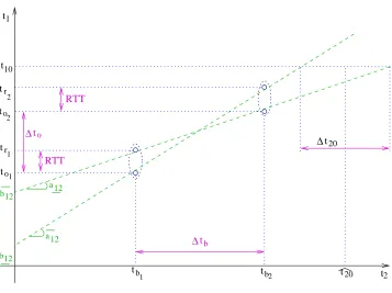
3.1 A probe message from node1is immediately returned by node2and time-stamped at each send/receive point resulting in the data-point (to, tb, tr). . . 27

3.2 The linear dependence (3.2) and the constraints imposed ona12andb12by three data-points. . . 28

3.3 A probe message from node1may be returned by node2after being time-stamped at both the send and receive points. . . 30

3.4 In this situation, after receiving data-pointA3−B3, tiny-sync will discard constraints A₂ andB2. However, after receivingA4 −B4, it turns out that the most constraining constraint would have beenA2−B4. . . 32

3.5 Setup for the simplified analysis of the algorithms. . . 35

3.6 Evolution of the uncertainty bound on the relative clock drifts∆a12as new data-points are received. . . 36

3.7 Evolution of the precision of∆t2mas more data-points are received. . . 38

3.8 Synchronization transitivity: ifsis synchronized with u, and u is synchronized withv, thensis synchronized withv. . . 39

3.9 Experimental setup. . . 41

3.10 Time-stamping in tiny-sync. . . 42

3.11 Sources of delay in the measurement process error. . . 43

3.12 Experimental setup for global synchronization. . . 44

(9)

3.14 Tiny-sync pairwise synchronization error. . . 46

3.15 Distribution of the synchronization errors. . . 46

3.16 Tiny-sync global synchronization error. . . 47

3.17 Synchronization errors as a function of the number of points considered for the linear fit and tiny-sync. . . 48

3.18 Comparison of synchronization errors as a function of the number of hops. . . 49

3.19 Comparison of synchronization errors as a function of the synchronization interval. . . 50

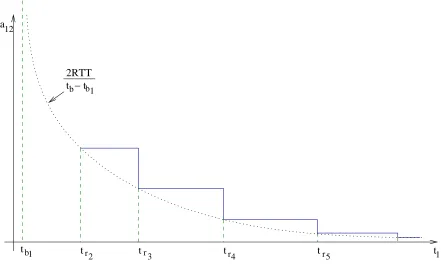
3.20 Behavior of tiny-sync when the clocks are forced to change their relative clock drift by sudden changes in the temperature of one of them (by temporary placing it in an ice-box). During the cool-down and warm-up period, tiny-sync restarts several times. (a) the evolution of the bound on the relative drift∆a12and the predicted evolution (3.23); (b) the evolution of the bounds on the drift. . . 50

3.21 The synchronization error when nodes were subjected to variation of the relative drift. . 51

3.22 The synchronization error with packet loss. . . 52

3.23 Synchronization error of tiny-sync and mini-sync as a function of the number of hops. . 52

3.24 Synchronization error of tiny-sync and mini-sync as a function of the synchronization interval. . . 53

3.25 Synchronization error of tiny-sync on Mica2 and Telos platforms. . . 54

3.26 Synchronization errors of tiny-sync without poor initial data. . . 55

3.27 Synchronization errors of tiny-sync when the best two out of the first ten data-points are used to initialize the algorithm. . . 55

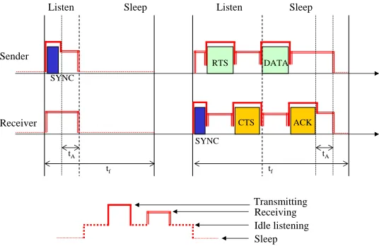
4.1 An example of a WSN topology. . . 63

4.2 Example of data exchange in 802.11 in ad-hoc mode without power saving. . . 65

4.3 Example of data exchange in 802.11 power saving mode (ad-hoc). . . 67

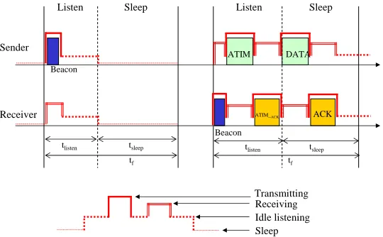
4.4 Example of data exchange in S-MAC. . . 70

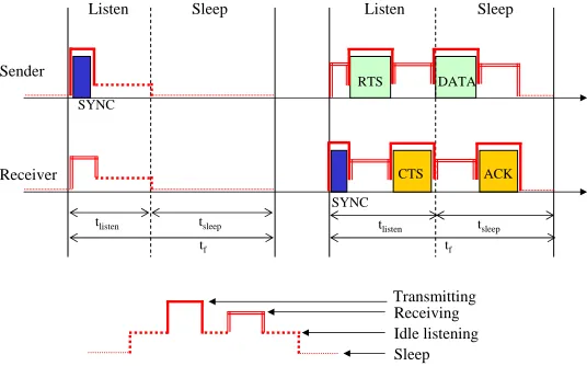
4.5 Example of data exchange in T-MAC. . . 71

4.6 Example of data exchange in B-MAC. . . 73

4.7 Comparison of the timelines between B-MAC and X-MAC [1]. . . 75

4.8 SCP-MAC synchronization scheme. . . 77

4.9 Example of data exchange in I-MAC. . . 79

4.10 Lifetime of the network as a function of the number of sensor nodes for Mica 2 and Telos motes (at constant network area). . . 83

4.11 Components of the power consumption of the first-tier of nodes as a function of the number of sensor nodes with constant deployment area for Mica2. . . 84

4.12 Components of the power consumption of the first-tier of nodes as a function of the number of sensor nodes with constant deployment area for Telos motes. . . 85

4.13 Lifetime of the network as a function of wake-up (check) interval for Mica 2 and Telos motes. . . 86

4.14 Components of the power consumption of the first-tier of nodes as a function of the wake-up interval for Mica 2. . . 87

4.15 Components of the power consumption of the first-tier of nodes as a function of the wake-up interval for Telos 2. . . 88

4.16 The radio state diagram and log messages. . . 90

(10)

4.18 Comparison of time and energy consumption of S-MAC between the analytical and

experimental results. . . 92

4.19 Comparison of time and energy consumption of 802.11 power-saving mode between the

analytical and experimental results. . . 92

4.20 Comparison of time and energy consumption of 802.11 basic mode between the

analyt-ical and experimental results. . . 93

4.21 Comparison of time and energy consumption of B-MAC between the analytical and

experimental results. . . 93

4.22 An example of DATA packet collision. . . 97

4.23 Lifetime of the network as a function of the number of sensor nodes for Mica 2 and

Telos motes (at constant network area). . . 98

A.1 Illustration for Lemma 7. . . 110

(11)

List of Tables

4.1 Current consumption and time for Mica2 radio operations . . . 81

4.2 Current consumption and time for Telos radio operations . . . 81

(12)

Chapter 1

Introduction

In this chapter, we first present the characteristics and applications of wireless sensor

net-works. We then explain why the power management is important in these netnet-works. Finally, we present

our contributions in this area.

1.1 Wireless Sensor Network

With the technology development of micro electronic mechanical systems (MEMS), wireless

communication, and embedded microprocessors, wireless sensor networks (WSNs) have been deployed

in environment monitoring, military target detection, and commercial areas [2–4]. Wireless sensor

networks usually consist of thousands of sensor nodes that are capable of sensing, processing, and

communicating. In typical sensor network applications, each sensor node obtains data from the physical

environment and transmits in wireless multihop fashion the data to the base station where the data will

be delivered to users through infrastructures such as Internet.

Although more than 90% of sensors are still wired, wired sensor networks have been replaced

by wireless sensor networks due to the cost and delay of deployment [5]. The dominant factor of

con-structing wired sensor networks is the wiring cost [6]. In addition, wired networks require considerable

time to implement. In case of wireless sensor network, the deployment is rather simple, in many cases,

just dropping off sensor nodes from the airplane into the target area instead of wiring from the target

area to monitoring station.

(13)

systems to obtain and process data from physical world. In environment monitoring, one of the

ear-liest applications of wireless sensor network, wireless sensors are used to monitor animals and plants

in wildlife habitat such as the Great Duck Island experiment [7]. Other related applications include

monitoring of water pollution, wildfires, and earthquakes. In the military battlefield, where there is

no infrastructure and it is very hard to access and deploy the sensor networks, the wireless sensor

net-works can be rapidly deployed to detect the enemy target and to track their movements in realtime.

Commercial applications include the monitoring and tracking of assets, monitoring of the conditions

of industrial equipment, automated meter reading, and warehouse management using RFID

technolo-gies. Wireless sensor networks can also be used in structural health monitoring of large structures such

as airplanes, buildings, and bridges. With the dedicated short range communication (DSRC) standard,

car-to-car networking with sensors can be available to provide emergency warning, traffic monitoring,

and driver safety assistance. One of the most important area of wireless sensor network applications is

health monitoring of patients in a hospital.

1.2 Power Management in Sensor Networks

Wireless sensor networks are similar to wireless ad hoc network in terms of networking

topol-ogy and multi-hop routing. But, sensor networks are also different from other wireless ad hoc networks

in that they consist of hundreds or thousands of autonomous nodes and the direction of most sensor

traffic is from the sensor nodes to the base station. Another unique characteristics of wireless sensor

networks is that the sensor nodes in WSNs are equipped with batteries of limited capacity and are

ex-pected to operate without human interaction for a long time. Therefore, the power management of each

sensor node plays a very important role in increasing the lifetime of the sensor networks [8]. For

ex-ample, when a Telos mote equipped with 2250mAh batteries idles without any power saving algorithm,

the mote can operate for up to 52 days. With a 1% duty cycle, the lifetime of the node can be extended

to 4076 days [9].

Recently, power management has been extensively studied in each area of sensor networks

such as the transmission power expenditure, medium access control (MAC) layer techniques, power

aware routing algorithms, network architecture, and sensor node deployment. The transmission power

(14)

connec-tivity. MAC layer techniques aim to conserve battery power by turning the receiver off whenever it is not

needed. Power aware routing algorithms seek to choose routes in such a way to maximize the lifetime of

the network by minimizing radio power consumption. Scheduling sensor nodes where each node goes

to power saving mode as long as possible can also save power consumption significantly by reducing

idle-listening time. The choice of the network architecture design (homogeneous or heterogeneous; flat

or hierarchical; the number of base stations; static or mobile access point) and node deployment policy

(node connectivity) can also affect the power management schemes.

In this dissertation, we explore the power management in WSNs in the following areas:

rout-ing, time synchronization, and MAC protocols. The most energy consuming part among sensor node

operations is the radio transmission and reception. Therefore, reducing the number of message

trans-missions and receptions for the functions that require message exchanges is imperative to minimize the

power consumption a sensor node. Routing is one of the those functions since the routing algorithms

exchange information with neighboring nodes to find the best route.

The nodes in sensor network are a distributed system. That is, each sensor node has its own

processing unit, memory, transceiver, and clock. In such a system, time synchronization between nodes

in the network is necessary in order for the sensor nodes to perform cooperative jobs such as target

tracking and reporting of time-sensitive data. All time synchronization protocols are based on message

exchanges between sensor nodes(either one or two ways). Thus, time synchronization is also an essential

function for the power management of wireless sensor networks.

Without power efficient MAC protocols, sensor nodes would listen to the network at all time

in order to receive messages from other nodes. This idle listening consumes a large percentage of the

energy of sensor nodes (Tables 4.1 and 4.2). Therefore, in order to minimize the energy consumption,

sensor nodes should be in sleep mode (or lower power mode) as long as possible and to be awake when

only necessary.

Time synchronization, routing, and power efficient MAC protocols are closely related to each

other as shown in Fig. 1.1. Many power efficient MAC protocols require accurate time synchronization.

If the sensor nodes are appropriately scheduled, the MAC contention can be reduced, which leads to a

lower number of message exchanges for routing and time synchronization. Global time synchronization

also needs power efficient routes from sensor nodes to the base station. The number of messages that a

(15)

Figure 1.1: Interactions between the power management modules in this thesis.

efficient MAC protocols.

1.3 Contributions

Power management plays a very important role in wireless sensor networks because most

sensor network applications operate on batteries and the deployment environments can be remote or

hostile. Power management in sensor networks is performed by considering all aspects of these networks

from the physical to the application layers, and even cross-layer. Our contributions in this field focus

on the areas of power aware routing, time synchronization, and analysis of power consumption of WSN

MAC protocols.

Power Aware Routing

In this area, we discuss the effect of power efficient routing algorithms on the lifetime of

mul-tihop wireless sensor networks. We assume that all data and control traffic in the network is flowing

be-tween the sensor nodes and the base station. This assumption results in a considerably simpler problem

and solution than for the more general MANETs. We analytically derive the maximum and minimum

bounds of the lifetime of the sensor network under specific routing algorithms. We also present the

routing algorithms that result in the maximum and minimum lifetime. We observe that the choice of

the routing algorithm has almost no consequence to the lifetime of the network. The simulation results

(16)

Time Synchronization

In this area, we present two simple and accurate pairwise time synchronization protocols for

wireless sensor networks. The two algorithms have the following features:

• Deterministic bounds on the precision: Most other algorithms provide best estimates for the offset

and drift of the clocks, and possibly probabilistic bounds on these estimates. Our approach

deliv-ers tight, deterministic bounds on these estimates, such that absolute information can be deduced

about ordering and simultaneous events.

• Accuracy: The experimental results show that pairwise time synchronization errors of proposed

algorithms are less than 1.5µs.

• Low computation and storage complexity: Wireless sensor nodes typically feature low

tional power microprocessors with small amounts of RAM. Both algorithms have low

computa-tional and storage complexity.

• Low sensitivity to communication errors: Wireless communications are notoriously error prone,

and thus one cannot rely on correct receipt of all messages. The presented approach works

cor-rectly even if a large percentage of the messages is lost.

We analytically derive deterministic bounds on offset and clock drift. The analytical results

show that the bounds on offset and clock drift only depend on the round trip times of messages between

two nodes.

Based on pairwise synchronization, we propose a method for synchronizing the entire

net-work. Performing global synchronization does not require extra effort on sensor nodes, but is done

implicitly by the pairwise synchronization. Proposed algorithms guarantee that the global

synchroniza-tion errors only depends on the number of hops between two sensor nodes.

We implemented proposed algorithms on Mica2 and Telos motes, measured the time

synchro-nization errors, and compared our results with other typical synchrosynchro-nization protocols.

(17)

• To minimize the measurement errors, we measured the time synchronization errors by wiring the

target sensor nodes into the measuring node and having the nodes report local times-tamps at the

same time by wired interrupts.

• We showed how the synchronization intervals affect the performance of time synchronization

protocols

• We showed that proposed algorithms are robust to unreliable wireless sensor networks.

Analyzing Power Consumption of WSN MAC protocols

We constructed a common power consumption model to be used heterogeneous MAC

pro-tocols. The power consumption model can represent the power consumption behavior of each MAC

protocol at the very detail level. We determined analytically the power consumption of the following

protocols:

• 802.11 basic mode

• 802.11 power-saving mode

• S-MAC

• T-MAC

• B-MAC

• X-MAC

• SCP-MAC

We performed the simulation using the analytical results and compare MAC protocols. With

the simulation results, we conclude that B-MAC and X-MAC are appropriate for the applications that

require short delay while S-MAC, T-MAC, or SCP-MAC should be used for monitoring applications

that tolerate long delays. We validated the analytical results by measuring energy consumptions of the

MAC protocols on a testbed using Mica 2 motes and compare the results. The experimental results show

(18)

Chapter 2

Power Aware Routing

In this chapter, we discuss the effect of power efficient routing algorithms on the lifetime

of wireless sensor networks. We calculate analytically lifetime bounds of the network under specific

routing algorithms. We perform the simulations to verify the analytically derived lifetime bounds.

2.1 Introduction

The power management problem for wireless sensor networks has been studied intensively.

Various approaches for reducing the energy expenditure have been presented in literature. In this work,

we focus on routing strategies that maximize the lifetime of the wireless sensor networks

Several strategies are commonly employed for power aware routing in WSNs [10]:

• Minimizing the energy consumed for each message. This metric might unnecessarily overload

some nodes causing them to die prematurely.

• Minimizing the variance in the power level of each node. This is based on the premise that it is

useless to have battery power remaining at some nodes while others exhaust their battery, since

all nodes are deemed to be equally important.

• Minimizing the cost/packet ratio In this approach, different costs can be assigned to different links,

for example, incorporating the discharge curve of the battery, and thus postponing the moment of

(19)

• Minimizing the maximum energy drain of any node. The basis of this approach is that the network

utility is first impacted when the first node exhausts its battery, and thus it is necessary to minimize

the battery consumption at this node.

The above approaches focus on different metrics of energy efficiency. A common

character-istic of these metrics is that they can lead to a disconnected network with a high residual power: once

the critical nodes of the network have depleted their batteries, the network is essentially dead. Indeed

we show that under our assumptions this is inevitable. For a practical sensing application, the network

can be considered to have stopped working when it fails to deliver the sensed readings from a bulk of

the sensors, and the important metric is the time when this occurs. In what follows, we will therefore

use the network lifetime as our main performance measure, which we define in the next section.

While all the above approaches provide benefits in different classes of MANETs, the special

case of WSNs merit closer evaluation since they are practically an important class of MANETs.

Gen-erally, the problem of computing the optimal lifetime of the MANETs is known to be hard due to node

mobility. As a special case of MANETs, the WSNs are (in most sensing applications) stationary and

have a base station sink, where all data traffic ends. In this work, we will derive bounds on the lifetime

of WSNs. We show that the two characteristics mentioned above play a crucial role in these

considera-tions. Somewhat surprisingly, we are able to show that network behavior under these conditions is quite

specific, the maximum benefit obtainable from the batteries is very predictable, and achievable by rather

simple routing strategies.

2.2 Related Work

Sensor Protocols for Information via Negotiation (SPIN) [11] makes good the deficiencies of

classic flooding by negotiation and resource adaptation. Using SPIN routing algorithm, sensor nodes

can conserve energy by sending the metadata that describes the sensor data instead of sending all the

data. SPIN can reduce the power consumption of individual node, but it may decrease the lifetime of

the whole network due to extra messages.

Low-Energy Adaptive Clustering Hierarchy (LEACH) is a clustering-based protocol that

min-imizes energy dissipation in sensor networks [12]. LEACH randomly selects sensor nodes as

(20)

nodes in the sensor network. LEACH can suffer from the clustering overhead, which may result in extra

power depletion.

The algorithmmax−min zPmincombines the benefits of selecting the path with the

min-imum power consumption and the path that maximizes the minimal residual power in the nodes of the

network [13]. However, this algorithm has the disadvantage of being centralized and requiring

knowl-edge of the power level of each node in the system. Its distributed version also has clock synchronization

problem.

Mhatre et al. [14] obtained the minimum number of sensor nodes, cluster heads, and battery

energy to ensure at least T unit of lifetime. They assume two types of sensor nodes: node 0 is sensor

node and node 1 is cluster head. The main result is that the number of cluster heads should be the order

of square root of the number of sensor nodes. They don’t give exact formula for the maximum lifetime

of the network. And, it is difficult for the assumption that cluster heads directly communicate with the

base station to be applied to general applications. They observed that the nodes close to the cluster heads

have high energy burden due to relaying of packets. But, one of their important observations, the sharp

cutoff effect, to maximize the lifetime does not hold at all time.

Bhardwaj et al. [15] computed the upper bound of active lifetime in terms of the routing

algorithms. But they did not consider that the first tier nodes determine the lifetime of the whole network.

They measured the lifetime of the network as the time of first loss of the coverage. That is, they did not

care the connectivity. [16] elaborated their work in [15] by taking into account the data aggregation and

random topology.

Zhand and Hou [17] presented necessary and sufficient condition for k-coverage. They also

derived the upper bound of the lifetime of all algorithms that select working nodes can achieve. They

included data transmission, reception, idle listening time, sensing, and data processing as the power

consumption of a node. They measured the lifetime of the network as -portion of coverage based on the

assumption that if transmission range is as twice as sensing range, coverage implies the connectivity.

Their work is different from ours because they derived the maximum lifetime of the network in terms of

nodes selection. And they did not consider the properties of the first nodes.

Pan et al. [18] observed the property that the first tier nodes are important for the lifetime of

the whole network. They provided approaches to maximize the topological lifetime of the network in

(21)

in clusters.

Alonso et al. [19] found explicit bounds on the minimal and maximal energy for routing

algorithms and used the bounds to derive the lifetime of the network. But the maximum lifetime of the

network derived by [19] is very similar to the minimum lifetime of the network derived by our approach.

The previous work on power aware routing algorithms focused on how to find the correct route

efficiently or how to enhance the lifetime of the network. In this work, we derive the lower and upper

bounds on the lifetime of the network in terms of the routing algorithms. That is, we give the answer for

the question that what is the maximum lifetime of the WSNs that routing algorithms can achieve. We

will also present the routing algorithms that show the maximum and minimum lifetime.

2.3 Definitions, Notations, and Assumptions

In this section, we define the lifetime of the network (the metric for determining the optimality

of routing algorithms). We also present the assumptions and notations used in the following sections.

2.3.1 Definitions

The lifetime of the networkLis the lifetime of the set of all its initial nodes.

2.3.2 Assumptions

We believe that the following assumptions apply to a large class of sensor network

implemen-tations and applications.

We assume that:

A-1 all network nodes are stationary,

A-2 all sensed data is sent to the base station (i.e. no filtering or other in-network processing is

performed),

A-3 all network nodes generate packets periodically with a common constant period,

A-4 the transmission range and transmission power is constant for all transmissions from all nodes,

(22)

A-6 there are more nodes in tieri+ 1than in tieriexcept for the last tier of nodes. (In terms of the

notation we introduce in section 2.3.3Ni+1 ≥Ni,1 ≤i≤H−2.) If this assumption holds at

deployment time, it will continue to hold for the lifetime of the network since the inner tiers carry

more traffic that the outer tiers and, thus, more nodes die in the inner tiers than in the outer tiers.

A-7 the traffic forwarding load from nodes which are more thanihops from the base station is equally

shared by all nodes which areihops from the base station.

Of the above, the first two are the crucial ones we mentioned before. The next two assumptions

merely represent a realistic case, and also simplify what follows, but do not reduce the scope of our

results. A-5 also represents a quite realistic condition; the removal or relaxation of this assumption is

not considered within the scope of this paper. A-6 is satisfied for most reasonable distribution of sensor

nodes, for example approximately uniform distribution over a large area. The assumption of a uniform

distribution is stronger than A-6 and is not needed for this paper. The main purpose of the minimal

assumption A-6 is to eliminate pathological cases where the WSN becomes prematurely disconnected

due to a bottleneck in the topology. Finally, A-7 is made for explanatory purposes and later we examine

the consequences of removing this assumption.

2.3.3 Model and Notations

We model the power consumptionP of a wireless node as:

P =PaT +Pb, (2.1)

where T is the number of flows transmitted by the node (comprising its own sensed data and data

forwarded on behalf of other nodes),Pais the power consumption used to forward the data in each flow,

andPb is the power consumption independent of the forwarded traffic. A sensor node that consumes

the same power independent of the number of flows forwarded is likely a wasteful node. A power

efficient sensor network has a very small Pb (mainly due to routing overhead, synchronization and

other middleware services), practically all its power being expended in useful sensing and forwarding of

information. In WSNs the traffic from the base station to the sensor nodes (queries, control information,

etc.) is usually broadcast and hence contributes toPb rather than toPa. The choice of the MAC layer

(23)

reducedPa andPb. Beyond the particular values of Pa andPb, the choice of the MAC layer is not

relevant for the reminder of this paper.

Regardless of its value, for our purposes,Pbdoes not play a role in the contribution of routing

to the network lifetimeL: simply by offsetting the initial battery level by a constant quantity (PbL) we

can compute the same lifetimeLby using a simplified model for the power consumption of a node:

P =PaT. (2.2)

We will use the following notation:

β is the energy spent to transmit one packet once.

p is the number of packets generated by each node in every second (thus, the energy spent every

second by each node to generate or forward one flow isβ p).

b is the initial battery level of every node (as discussed only the battery expended for forwarding

and sending its own data is relevant for the network lifetime).

H is the maximum number of hops between the base station and any of the wireless nodes in the

WSN.

N is the set of all sensor nodes.

Ni is the set of sensor nodes that are at a minimum ofihops away from the base station. We also call

this set of nodes theith tier of nodes. For example, the first tier of nodes consists of the nodes

that can directly reach the base station. With our assumptions, initially all nodes of inNiwill also

be exactlyihops from the base station; however, as nodes in Ni−1 die, some nodes inNi may

require more thanihops to reach the base station, and become part of the setNi+1. However,

note that nodes inN1never migrate to other tiers.

N is the total number of sensor nodes;N =|N |.

Ni is the number of nodes in tieri;Ni =|Ni|.

T_ir(n) is the number of packets transmitted by noden∈ Niusing the routing algorithmr.

(24)

Lr

i is the lifetime of the nodes ofNiwhen using routing algorithmr.

R is the set of all minimum hop routing algorithms able to find a path between each sensor node and

the base station if such a path exists. Usually, each node in the setNi has multiple shortest hop

neighbors in the setNi−1; The choice of one of these neighbors (e.g. randomly, or based on the

residual power) differentiates among the algorithms inR.

2.4 The effect of the routing algorithms on the lifetime of the WSN

When the traffic pattern in a network is such that all nodes transmit to an egress node such as

a base station, the few nodes that can reach the base station directly will be responsible for the highest

amount of traffic forwarding. We have examined this phenomenon in detail in [30], below we present

the result that is relevant to us in the current context. Then we use this result to obtain lower and upper

bounds for the lifetime of the network as a function of the routing protocol.

Lemma 1 For any routing algorithmr ∈ R, the lifetime of the nodes inN1 is equal to the lifetime of

the nodes in other tiers (Ni, i > 1). In other words,Lr1 =Lri for alliandrsuch that1 < i≤Hand

r∈ R.

Proof For allr∈ Randi >1,

X

n∈N1

T₁r(n)> X

n∈Ni

T_ir(n) (2.3)

because there are no loops in the paths through the nodes in tieriand, hence, the traffic in the first tier

of nodes includes the traffic from any other tier (and adds its own traffic). Using either (2.1) or (2.2) this

implies that the power consumption of nodes in the first tier is higher than that of the nodes in any other

tier. Since all nodes have the same initial battery size (assumption A-5) and there are more nodes in tier

ithan in tier 1 (assumption A-6), the nodes in the first tier will deplete their battery strictly sooner than

the nodes in any other tier. However, as soon as the first tier of nodes depletes its batteries, the entire

network becomes disconnected (and by the definition of the lifetime in Section 2.3.1 all tiers reach their

(25)

Theorem 2 For a WSN satisfying all assumptions in Section 2.3.2 and using a routing algorithmr ∈ R

the lifetime of the network is

Lmin = _{N βp}N1b. (2.4)

Proof According to Lemma 1, the lifetime of the network is determined by the lifetime of the first tier

of nodes. Considering assumption A-7, every node in the first tier will expend the battery at the same

(constant - assumption A-3) rate. Further, each flow originating from outside of tier 1 is forwarded by

exactly one first tier node: since tier 1 nodes are the only nodes that can transmit directly to the base

station. Each first tier node also originates exactly one flow of its own. Finally, considering that all

nodes have the same initial battery (assumption A-5), all nodes in the first tier will deplete their battery

at the same time. The moment when the first (and last) battery is depleted coincides with the time of the

death of the network. Thus, the battery expended on the first tier of nodes is used to forward data for all

nodes in the network for the duration of the networks’ lifetime:

N₁b=L_minN βp. (2.5)

The above is valid if all nodes are alive until the lifetime expires, as will happen if the load

balancing assumption A-7 strictly holds. However, this will not hold in practice because the node

positions may have some asymmetry. We next examine the consequence of removing the assumption.

To distinguish, we shall refer to the ideal routing situation where the assumption A-7 is perfectly met as

Load Balanced Shortest Path First (LBSPF).

We focus on the first tier, since we know the lifetime is defined by these nodes. If

assump-tion A-7 is not satisfied in the first tier, then all nodes of the first tier will not die at the same time. The

lifetime of the network will be defined by the first tier node which dies last. However, before this time,

the number of first tier nodes still alive has declined slowly. The number of nodes that remain alive

in the first tier at any given time affects the total traffic generated by the first tier itself. Initially, the

total battery amount of first tier nodes isN1b. For each period, the first tier consumes an energy equal to

Naliveβp, whereNaliveis the number of active nodes in the network. A routing algorithm can maximize

the lifetime of the network if it can reduceNaliveas soon as possible. A practical way to quickly reduce

the number of nodes that are alive is to overburden a node until its battery is depleted. Thus, the routing

(26)

battery. After nodex1dies, another node from the first tier,x2, is selected to carry all the network flows,

and so on until the last node in the first tier dies (at which time the network becomes disconnected).

We shall refer to this rather curious routing approach as Bottleneck Routing (BR). While BR does not

belong in the setR(not all nodes in tier 2 may be able to reachx1in one hop), it represents the extreme

limit of unbalanced routing protocols inR. Thus all protocols inRwill result in a network lifetime

bounded by those achieved by LBSPF and BR, from below and above respectively.

In LBSPF, the base station will receive readings from all nodes for the entire lifetime. This is

no longer true for BR, some nodes will die and stop reporting before lifetime expires. While this may

be a problem from the sensing application’s perspective, we show below that it improves the lifetime of

the network as we defined it earlier.

Theorem 3 If we remove assumption A-7, the maximum lifetime of a WSN using a routing algorithm

r∈Ris bounded byL < Lmax, where

Lmax= _βpb

"

1−

µ

1− 1

N −N1+ 1

¶_N₁#

(2.6)

Proof As discussed above, the lifetime is composed of different periods when the different nodes of the

first tier will take turns forwarding all traffic from outside the first tier. To compute the lifetime of the

network we simply add the times it takes for all nodes in the first tierx1, x2, . . . , xn1 to die:

• nodex1 will carry the flows on behalf ofN −N1 nodes and its own flow. Thus it will die after

t1= ₍_N₋_Nb₁₊₁₎_βp.

• nodex2will carry only one flow for timet1 and then the same number of flows as nodex1, and

hence will die aftert2seconds after the death ofx1:t2 = ₍_N₋b−_Nt₁1₊₁₎βp_βp.

.. .

• nodexN1 will dietN1 seconds after nodexN1−1 died, wheretN1 =

b−PN1−1

i=1 tiβp

(N−N1+1)βp.

Thus,

L_max=

N1

X

i=1

t_i. (2.7)

Equation (2.7) can be further manipulated by noticing thatti =t1(1−_N₋_N1₁₊₁)i−1for alli

(27)

Comments:

• LBSPF and BR are the two extreme approaches to routing in WSNs. LBSPF ensures that the time

of the death of the first node is postponed as much as possible. On the other hand, BR postpones

the time of the disconnection of the network as much as possible. Any minimum hop routing will

result in routes that will fall between these two extremes, hence so will the lifetimes.

• Figure 2.1 depicts the difference in the network lifetimes of the two approaches as a function of

the total number of nodesN over the number of nodes in the first tierN1. For this figureN1 was

kept constant at 100 nodes whileN increased from 200 nodes to 2500 nodes. It is interesting to

see that the difference between the two extremes becomes very small as total number of nodes

becomes large in comparison to the number of nodes in tier 1.

• Bottleneck Routing maximizes the lifetime of the network at the expense of purposely

deplet-ing some of the nodes relatively early. For most applications it is unlikely that this is desired,

especially since, for large networks, the savings in the lifetime are insignificant (Fig. 2.1). This

observation makes the definition of optimal WSN routing protocols that use only the lifetime as

an optimization criteria questionable.

0 5 10 15 20 25 0.75

0.8 0.85 0.9 0.95 1

N/N₁

Lmin /Lmax

Figure 2.1: Lifetime ratios using LBSPF and BSPF as a function of the ratio between the total number of nodes and the nodes in tier one.

It is clear that for all possible routing algorithms in R the lifetime L of the network falls

(28)

close to each other especially for large networks. Therefore it can be claimed that the choice of the

routing protocol does not make a significant difference in the lifetime of the network. For example, in a

uniformly distributed WSN with five tiers the difference between the two lifetimes is less than 2%.

It is likely that a simple protocol will perform just as well as a more complex protocol. The

only major differentiation between different routing protocols is in their overhead (included inPb in

(2.1)).

2.5 Simulation Results

To validate the results in Section 2.4 we simulated a WSN of variable size with two routing

algorithms.

We have implemented two versions of Shortest Path First (SPF) algorithms to compare the

lifetime of WSN using these algorithms with the theoretical limit:

MSPF The algorithm selects among the neighbors with the same number of minimum hops to the base

station the one with the largest remaining power. Essentially this algorithm behaves very like

Load Balancing SPF ensuring that all nodes in the first tier die at (almost) the same time.

RSPF The algorithm selects randomly among the neighbors with the same number of minimum hops to

the base station.

We reroute (choose new routes for all nodes) periodically (every one time unit) or whenever a

node dies.

We fixed the node density at (0.01nodes/m2_{) and the transmission radius of the nodes (}₃₀_m_).

The transmission of the data generated by a node each time unit costs one unit of energy. The nodes

initially have 1000 units of energy. All simulations were repeated thirty times with different random

seeds; in what follows, the average of these results is presented.

Figures 2.2 and 2.3 depict the variation of the network lifetime with the network size (constant

density) for uniform (we used a rectangular grid) and random placement respectively. The lifetimes of

network using the two versions of SPF algorithms are very close together and between the theoretical

values given by (2.4) and (2.6). The lifetime are so close that they are hard to tell apart from each other.

(29)

100 200 300 400 500 600 700 800 900 102

Number of nodes

Lifetime

L

max

L

min

MSPF RSPF

Figure 2.2: Variation of the lifetime of the network for a rectangular grid placement as a function of the networks size

100 200 300 400 500 600 700 800 900 102

Number of nodes

Lifetime

L

max

L_min MSPF RSPF

(30)

0 20 40 60 80 100 0

10 20 30 40 50 60 70 80

Time

Number of dead nodes

L max L

min MSPF RSPF

Figure 2.4: Time of death for each node for various routing strategies for an uniform rectangular grid placement.

the significant variation introduced by the random initial topology. Figure 2.3 also depicts the 95%

confidence interval corresponding to the average lifetimes. The lifetime of the network decreases as the

number of sensor nodes increases: a fixed number of tier one nodes carry increasingly more packets

and, hence, naturally die sooner.

Figures 2.4 and 2.5 show the moment of death of each node in the first tier of the network.

For the two limits corresponding to Lmin and Lmax we depicted the times when first tier nodes are

expected to die following the LBSPF and BR algorithms. For this simulation we usedN = 400nodes

in an area190m×190m. MSPF for the grid network works as expected: practically all nodes of the

networks are alive for the entire lifetime of the network. For the random placement scenario, MSPF

works reasonably well, but less so than in the case of the uniform grid. The main reason behind this

behavior is that in the case of random placement there might not be possible to balance the load, and

inevitably some nodes will die sooner than others. The number of disconnected nodes spikes abruptly

when the network becomes disconnected, i.e. when the network reached its lifetime. As expected, for

both placements, the lifetime of RSPF is slightly larger than for MSPF at the expense of the early deaths

(31)

0 10 20 30 40 50 60 70 80 0

10 20 30 40 50 60 70 80

Time

Number of dead nodes

L max L

min MSPF RSPF

Figure 2.5: Time of death for each node for various routing strategies for a random placement.

2.6 Conclusion

In this chapter we presented an analysis of the lifetime of wireless sensor networks that employ

periodic sensing. Lower and upper bounds on the network lifetime are derived, and corresponding

routing algorithms leading to these bounds are presented. For large sensor networks the upper and the

lower bounds on the network lifetime are relatively close (less than a few percents), leading thus to

the conclusion that for such sensor networks the choice of the routing protocol is largely irrelevant for

maximizing the network lifetime, as long as some form of shortest paths are followed. Simulations are

used to validate the theoretical results.

While the setRmay appear to be rather restrictive, in reality our results are likely to continue

to hold for many sensible routing approaches. We are currently working on developing descriptions of

(32)

Chapter 3

Time Synchronization

3.1 Introduction

Recent technological advances in low power radios, sensors and microcontrollers enable a new

monitoring paradigm for large geographical areas. The vision involves a large number of inexpensive

nodes equipped with one or more sensors, a small microcontroller and transceivers capable of

short-range communications. Wireless sensor networks (WSNs) [2–4] have the potential to truly revolutionize

the way we monitor and control our environment.

Many (if not most) WSN applications either benefit from, or require, time synchronization.

Sensed data is typically forwarded over multiple hops to one or more base stations and encounters delays

ranging from a few tens of milliseconds to several minutes [31]. Many energy-efficient algorithms trade

power savings for increased delays. Therefore, without time synchronization, the time that sensed data

reached the base station is often a poor approximation of the time the data was sensed. If the entire sensor

network is time-synchronized (with respect to the base station), meaningful time-stamps can accompany

sensed data. Target tracking, one of the most popular sensor network applications, requires tight time

synchronization for beam-forming. Many WSN protocols (e.g., power-saving sleep schedules [32],

TDMA schedules for maximizing the networks’ capacity, security mechanisms for preventing replay

attacks, etc.) also rely on time synchronization.

In this Chapter, we present two closely-related algorithms suitable for pair-wise time

(33)

clock with respect to the one of the other node. We also present a scheme building on these algorithms,

which is capable of synchronizing the clocks of an entire sensor field. To avoid confusion between

the two algorithms, we will name them mini-sync and tiny-sync as they use limited and very limited

resources, respectively. The two algorithms feature:

• Drift awareness: The algorithms not only take the drift of the clock into account, but also find

tight bounds on the drift.

• Deterministic bounds on the precision: Most other algorithms provide best estimates for the offset

and drift of the clocks, and possibly probabilistic bounds on these estimates. Our approach

deliv-ers tight, deterministic bounds on these estimates, such that absolute information can be deduced

about ordering and simultaneous events.

• Precision: Given small uncertainty bounds on the delays exchanged messages undergo, the

pre-cision of the synchronization can be arbitrarily good.

• Low computation and storage complexity: Wireless sensor nodes typically feature low

tional power microcontrollers with small amounts of RAM. Both algorithms have low

computa-tional and storage complexity.

• Low sensitivity to communication errors: Wireless communications are notoriously error prone,

and thus one cannot rely on correct receipt of all messages. The presented approach works

cor-rectly even if a large percentage of the messages is lost.

The main contribution of the work is the development and performance evaluation of two

simple algorithms that deliver accurate offset and drift information together with tight bounds on them.

The two algorithms presented in this chapter are not limited to wireless sensor networks. They

can synchronize the nodes on any communication network which allows bidirectional data transmission.

However, the algorithms provide very good precision (microsecond if crafted carefully) and bounds on

the precision while using very limited resources, thus being especially well suited for wireless sensor

(34)

3.2 Related Work

Time synchronization is a key service for many applications and operating systems in

dis-tributed computing environments. Many protocols have been proposed and used for time

synchroniza-tion in wired and wireless networks. Mill’s Network Time Protocol (NTP) [33,34] has been widely used

in the Internet for decades. Nodes could also be equipped with a global positioning system (GPS) [35]

to synchronize them. However, traditional synchronization schemes and GPS-equipped systems are not

suitable for use in WSNs due to the specific requirements of those networks:

• Precision: Depending on the considered application, WSNs may require far better precision than

traditional networks. For example, a precision of a few milliseconds is considered satisfactory

for NTP, while in a WSN beam-forming application, microsecond precision can significantly

improve the performance of the application [36]. Furthermore, when coordinating synchronized

time schedules, the higher the precision of the synchronization algorithm, the smaller the guard

times have to be (and, hence, the higher the efficiency of the scheduling approach).

• Cost: Cost is of primary concern in WSNs as, typically, nodes have limited batteries,

computa-tional and storage resources. Most of the protocols designed for wired environments exchange

many messages for statistical processing. Furthermore, the protocols also need to store the

mes-sages to process them.

Recently, a significant amount of research on time synchronization for wireless sensor

net-works has been published [37, 38]. An interesting approach called post facto synchronization was

pro-posed by Elson and Estrin [39]. In this approach, each node’s clock is normally unsynchronized with

the rest of the network; a beacon node periodically broadcasts beacon messages to the sensor nodes in

its wireless range. When an event is detected, each node records the time of the event (time-stamp with

its own local clock). After the event (hence, the name), upon receiving the reference beacon message,

nodes use it as time reference and adjust their event timestamps with respect to that reference.

The reference broadcast synchronization (RBS) protocol [40], uses a data collection

mecha-nism similar to the one in the post facto synchronization: one node acts as a beacon by broadcasting a

reference packet. All receivers record the packet arrival time. The receiver nodes then exchange their

(35)

using a least-squares linear regression. The interesting feature of RBS is that it records the timestamp

only at the receivers. Thus, all timing uncertainties (including MAC medium access time) on the

trans-mitter’s side are eliminated. This characteristic makes it especially suitable for hardware that does not

provide low-level access to the MAC layer (e.g., 802.11). Although RBS synchronization only involves

one hop neighbors, the mechanism can be extended to synchronize a multi-hop network [41]. In such

a system, timestamps in messages can be reconciled as they are being forwarded by the intermediate

nodes (according to their next-hop destination and its time difference to the current node) [42]. The main

disadvantage of RBS is that it does not synchronize the sender with the receiver directly and that, when

the programmers have low-level access at the MAC layer, simpler methods (e.g., TPSN) can achieve a

similar precision to RBS.

R¨omer [43] presented a synchronization protocol for ad hoc networks. The authors assume

clocks with known upper-bounds on the clock drift. The basic idea of the algorithm is to compute

timestamps using unsynchronized local clocks. When a local time-stamp is transferred between two

nodes, the timestamp is transformed to the local time of the receiving node with guaranteed bounds

based on the assumed maximum clock drift. These protocols focus on temporal relationships between

the events such as ”event X happened before event Y” and ”event X and Y happened within a certain time

interval.” [44] enhanced R¨omer’s algorithm and achieved higher accuracy while reducing computation.

When implementing time synchronization protocols, significant challenge is minimizing

times-tamping uncertainties. RBS reduces these uncertainties by timestimes-tamping only at the receivers. The time

synchronization protocol for sensor network (TPSN) [45] reduces the uncertainties by using timestamps

at the medium access control (MAC) layer. This eliminates the (large) uncertainties introduced by the

MAC layer, e.g., retransmissions, backoffs, medium access, etc. TPSN takes advantage of the

avail-ability of the MAC layer code in TinyOS [46]. For a single beacon, TPSN offers a two-fold increase in

precision in comparison to RBS (although, asymptotically, as more beacons are sent, they achieve the

same precision ).

The Flooding Time Synchronization Protocol (FTSP) [47] was designed for a sniper

localiza-tion applicalocaliza-tion requiring very high precision [36]. FTSP achieves the required accuracy by utilizing a

customized MAC layer time-stamping and by using calibration to eliminate unknown delays. FTSP is

robust to network failures, as it uses flooding both for pair-wise and for global synchronization. Linear

(36)

of FTSP is that it requires calibration on the hardware actually used in the deployment (and thus, it is

not a purely software solution independent of the hardware). FTSP also requires intimate access to the

MAC layer for multiple timestamps. However, if well calibrated, the FTSP’s precision is impressive

(less than 2µs).

Lightweight Time Synchronization (LTS) [48] was proposed for applications where the

re-quired time accuracy is relatively low. The pair-wise synchronization on LTS is similar to TPSN except

for the treatment of the uncertainties (LTS adopts a statistical model for handling the errors). The

simu-lation results show that the accuracy of LTS is about 0.5 seconds.

Li and Rus [49] presented a high-level framework for global synchronization. The authors

proposed three methods for global synchronization in WSNs. The first two methods, all-node-based

and cluster-based synchronization, use global information and are, hence, not suitable for large WSNs.

In the third method (diffusion), each node sets its clock to the average clock time of its neighbors. The

authors showed that the diffusion method converges to a global average value. A drawback of this

approach is the potentially large number of messages exchanged between neighbor nodes, especially in

dense networks.

Dai and Han [50] proposed two time synchronization protocols, Hierarchy Referencing Time

Synchronization (HRTS) and Individual-based Time Request (ITR). HRTS uses an idea similar to RBS

except for the synchronization of the receivers after the beacon synchronization message was sent:

instead of the receivers exchanging messages among themselves, a designated node sends its time to the

beacon node that, in turn, broadcasts this message over the entire network, thus, significantly reducing

the number of message exchanges. Similar to RBS, the beacon node has to be able to broadcast to the

entire sensor network. The ITR protocol is based on NTP. Multichannel support is integrated both in

ITR as well as HRTS to reduce the delay variations.

Delay Measurement Time Synchronization Protocol (DMTS) [51] reduces the number of

mes-sage exchanges in RBS by accurately estimating the delay of the path from the sender to the receiver.

DMTS is similar to RBS on the sender side and TPSN or FTSP on the receiver side.

Adaptive Clock Synchronization [52] is a probabilistic method for clock synchronization that

uses the higher precision of receiver-to-receiver synchronization. The protocol extended the

determin-istic RBS protocol to provide a probabildetermin-istic bound on the accuracy of the clock synchronization. The

(37)

Su [53] proposed Time-Diffusion Synchronization Protocol (TDP) for network-wide time

syn-chronization. TDP maintains global time synchronization within an adjustable bound (based on the

ap-plication requirements). TDP achieves global synchronization by multi-hop flooding: the base station

initiates the protocol by sending a special timing message to the entire network. Some of the nodes,

upon receiving the message, become masters by using a leader election procedure (that uses a False

Ticker Isolation Algorithm to discard outliers and a Load Distribution Algorithm to balance the energy

consumption of the network). The master nodes start the time diffusion procedure involving electing

diffused leaders (similar to the master election algorithm), multi-hop flooding and iterative weighted

averaging of timing from different master nodes. TDP handles node mobility and failures by using a

Peer Evaluation Procedure. The method achieves a precision of 0.1s.

3.3 Proposed Algorithms

In this section, we present the two proposed algorithms and their expected performance.

3.3.1 Data Collection

For the proposed algorithms, we will use a classical data collection algorithm [33, 43, 45, 54,

55]; however, we will process the data differently.

Consider a wireless nodeiwith its hardware clockti(t), wheretis the Coordinated Universal

Time (UTC). In general, the hardware clock of nodeiis a monotonically non-decreasing function oft.

In practice, a quartz oscillator is often used to generate the real-time clock. The oscillator’s frequency

depends on the ambient conditions, but for relatively extended periods of time (minutes - hours), the

hardware clock can be approximated with good accuracy by an oscillator with fixed frequency:

ti(t) =ait+bi, (3.1)

whereai andbi are the drift and the offset of nodei’s clock. In general,ai andbi will be different for

each node and approximately constant for an extended period of time.

Consider two wireless nodes1and2with their hardware clockst1(t)andt2(t), respectively.

(38)

t1(t) =a12t2(t) +b12. (3.2)

The parametersa12andb12represent the relative drift and the relative offset between the two

clocks, respectively. If the two clocks are perfectly synchronized, the relative drift is equal to one, and

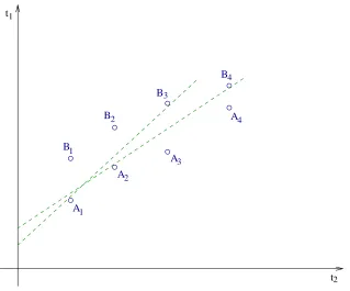
the relative offset is equal to zero.

Assume that node 1 would like to be able to determine the relationship betweent1 andt2.

Node1sends a probe message to node2. The probe message is time-stamped just before it is sent with

to. Upon receipt, node2time-stamps the probetband returns it immediately (we will shortly relax this

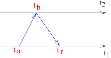
constraint) to node1which timestamps it upon receipttr. Figure 3.1 depicts such an exchange.

t

₁

t

₂

t o

t b

t r

Figure 3.1: A probe message from node1is immediately returned by node2and time-stamped at each

send/receive point resulting in the data-point (to, tb, tr).

The three time-stamps (to, tb, tr) form a data-point which effectively limits the possible values

of parametersa12andb12in (3.2). Indeed, sincetohappened beforetb, andtb happened beforetr, the

following inequalities should hold:

to < a12tb+b12, and (3.3)

tr > a12tb+b12. (3.4)

The data collection procedure described above is repeated several times; and each probe that

returns, provides a new data-point and, thus, new constraints on the admissible values ofa12andb12.

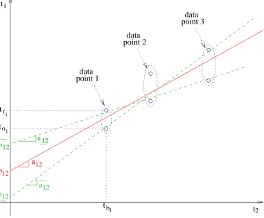
The linear dependence betweent1 andt2and the constraints imposed by the data-points can

be represented graphically as shown in Fig. 3.2. Each data-point can be represented by two constraints

in the system of coordinates given by the local clocks of the two nodest2 andt1. The double subscript

of the timestampstoi, tbi andtri denotes the timestamps corresponding to data-pointi. Inequality (3.3)

(39)

1

data

point 3data

point 1data t₁

t2 t_r

to

b₁₂

a₁₂

12

b 12

a 12 12

b

a

1

t_b

point 2

(40)

coordinates (tb, to). Similarly, corresponding to inequality (3.4), the line has to be under the point of

coordinates(tb, tr)(the second constraint). Satisfying both constraints, requires the line to be positioned

between the two constraints determined by each data-point. The exact values ofa12andb12cannot be

accurately determined using this approach (or any other approach) as long as the message delays are

unknown. But,a12andb12can be bounded by:

a12≤ a12 ≤a12, and (3.5)

b12≤ b12 ≤b12, (3.6)

wherea12 (a12) is the maximum (minimum) of the slopes of lines that satisfy the constraints, andb12

(b12) is the value on the y-axis at the intersection with the line corresponding toa12(a12).

Not all combinations ofa12andb12satisfying (3.5) and (3.6) are valid, but all valid

combina-tions satisfy (3.5) and (3.6). The real values ofa12andb12can be estimated as the midpoint of the range

of possible valuesac12andbc12:

a12 ∈

· c

a12−∆a₂12;ac12+∆a₂12

¸

, and (3.7)

b12 ∈

· c

b12−∆₂b12;bc12+ ∆b₂12

¸

, (3.8)

where

c a12 =

a12+a12

2 , (3.9)

∆a12 = a12−a12, (3.10)

c b12 =

b12+b12

2 , and (3.11)

∆b12 = b12−b12. (3.12)

The goal of the algorithms is to determinea12, a12, b12andb12as tight as possible (such that

it minimizes∆a12and∆b12). Oncea12andb12are estimated, node1can always correct the reading of

the local clock (using (3.2)) to have it match the readings of the clock at node2.

To decrease the overhead of this data-gathering algorithm, the probes can be piggy-backed on

data messages. Since most MAC protocols in wireless networks employ an acknowledgment (ACK)

scheme, the probes can be piggy-backed on the data and the responses on the ACKs. Elaborate schemes

(41)

be sent. This way, synchronization can be achieved almost “for free” (i.e., with very little overhead in

terms of communication bandwidth).

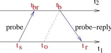
Relaxing the Immediate Reply Assumption

In Fig. 3.1, we assumed that node2replies immediately to node1when it receives a probe.

The correctness of the presented approach is not affected in any way even if node2does not respond

immediately. Node2can delay the reply as long as it wants; the relations (3.3) and (3.4), and, thus the

rest of the analysis will still hold.

However, as the delay betweentoandtrincreases, the precision of the estimates will decrease.

In practice, node2 may have to delay the reply due to any number of reasons (e.g., it has something

more important to send, it has to postpone its transmission due to medium access contention, etc.).

b

1 t2

tbr

t r t s t o

probe probe−reply

t

Figure 3.3: A probe message from node1may be returned by node2after being time-stamped at both

the send and receive points.

To counteract the possible loss in precision, node2can time-stamp the probe message upon

receipt (tbr) as well as upon reply (tb) (as depicted in Fig. 3.3). In this case, node 1 can adjustto as

follows:

to =ts+ac12(tb−tbr), (3.13)

whereto is the latest time at node 1 that is known to have occurred beforetb. The same inequalities

(3.3) and (3.4) hold for this case as well.

Increasing Precision by Considering Minimum Delay

If no information about delays encountered by the probe messages is available, nothing else

can be done to increase the precision. However, if the minimum delay a probe encounters between the

Power Management in Wireless Sensor Networks

Contents

List of Figures

List of Tables

Chapter 1

Introduction

1.1

Wireless Sensor Network

1.2

Power Management in Sensor Networks

1.3

Contributions

Chapter 2

Power Aware Routing

2.1

Introduction

2.2

Related Work

2.3

Definitions, Notations, and Assumptions

2.4

The effect of the routing algorithms on the lifetime of the WSN

2.5

Simulation Results

2.6

Conclusion

Chapter 3

Time Synchronization

3.1

Introduction

3.2

Related Work

3.3

Proposed Algorithms

t

t

t o

t b

t r