Scholarship@Western
Scholarship@Western
Electronic Thesis and Dissertation Repository
8-31-2016 12:00 AM
Molecular Distance Maps: An alignment-free computational tool
Molecular Distance Maps: An alignment-free computational tool
for analyzing and visualizing DNA sequences' interrelationships
for analyzing and visualizing DNA sequences' interrelationships
Rallis Karamichalis
The University of Western Ontario
Supervisor Prof. Lila Kari
The University of Western Ontario Graduate Program in Computer Science
A thesis submitted in partial fulfillment of the requirements for the degree in Doctor of Philosophy
© Rallis Karamichalis 2016
Follow this and additional works at: https://ir.lib.uwo.ca/etd
Part of the Other Computer Sciences Commons
Recommended Citation Recommended Citation
Karamichalis, Rallis, "Molecular Distance Maps: An alignment-free computational tool for analyzing and visualizing DNA sequences' interrelationships" (2016). Electronic Thesis and Dissertation Repository. 4071.
https://ir.lib.uwo.ca/etd/4071
This Dissertation/Thesis is brought to you for free and open access by Scholarship@Western. It has been accepted for inclusion in Electronic Thesis and Dissertation Repository by an authorized administrator of
In an attempt to identify and classify species based on genetic evidence, we propose a novel combination of methods to quantify and visualize the interrelationships between thousand of species. This is possible by using Chaos Game Representation (CGR) of DNA sequences to compute genomic signatures which we then compare by computing pairwise distances. In the last step, the original DNA sequences are embedded in a high dimensional space using Multi-Dimensional Scaling (MDS) before everything is projected on a Euclidean 3D space.
To start with, we apply this method to a mitochondrial DNA dataset from NCBI containing over 3,000 species. The analysis shows that the oligomer composition of full mtDNA se-quences can be a source of taxonomic information, suggesting that this method could be used for unclassified species and taxonomic controversies.
Next, we test the hypothesis that CGR-based genomic signature is preserved along a species’ genome by comparing inter- and intra-genomic signatures of nuclear DNA sequences from six different organisms, one from each kingdom of life. We also compare six different distances and we assess their performance using statistical measures. Our results support the existence of a genomic signature for a species’ genome at the kingdom level.
In addition, we test whether CGR-based genomic signatures originating only from nuclear DNA can be used to distinguish between closely-related species and we answer in the negative. To overcome this limitation, we propose the concept of “composite signatures” which combine information from different types of DNA and we show that they can effectively distinguish all closely-related species under consideration. We also propose the concept of “assembled signatures” which, among other advantages, do not require a long contiguous DNA sequence but can be built from smaller ones consisting of 100-300 base pairs.
Finally, we design an interactive webtool MoDMaps3D for building three-dimensional Molecular Distance Maps. The user can explore an already existing map or build his/her own using NCBI’s accession numbers as input. MoDMaps3D is platform independent, written in Javascript and can run in all major modern browsers.
free, chaos game representation, additive DNA signatures, Molecular Distance Maps
This thesis consists of three published articles. The article in chapter three was published in the journal PloS ONE, while the articles in chapter four and five were published in the journal BMC Bioinformatics. The author order follows the conventions of the field: For papers in chapter 4 and 5 the order is alphabetical; The paper in chapter 3 has two senior authors (LK, KAH) and the author order reflects the contributions of the authors. The major individual contributions are listed below.
Chapter 3 contains the article “Mapping the space of genomic signatures” by Lila Kari, Kathleen A. Hill, Abu S. Sayem, Rallis Karamichalis, Nathaniel Bryans, Katelyn Davis, Nikesh S. Dattani. The individual contributions are as follows. Analyzed the data: NB, KAH, NSD. Wrote the paper: LK. Designed the software: NB, NSD, RK, ASS. In-depth analysis: LK, KAH, ASS, RK, NB, KD, NSD.
Chapter 4 contains the article “An investigation into inter- and intragenomic variations of graphic genomic signatures” by Rallis Karamichalis, Lila Kari, Stavros Konstantinidis and Steffen Kopecki. The individual contributions are as follows. RK: data collection; data anal-ysis, methodology and result interpretation; manuscript draft; manuscript editing; software design. LK: data analysis, methodology and result interpretation; manuscript draft; manuscript editing. S.Kon: data analysis, methodology and result interpretation; manuscript editing. S.Kop: data analysis, methodology and result interpretation; manuscript editing.
Chapter 5 contains the article “Additive methods for genomic signatures” by
Rallis Karamichalis, Lila Kari, Stavros Konstantinidis, Steffen Kopecki, Stephen Solis-Reyes. The individual contributions are as follows. RK: data collection, data analysis, methodology and result interpretation, manuscript tables and figures, manuscript editing, software design and implementation. LK: data analysis, methodology and result interpretation, manuscript draft, manuscript editing. S.Kon: data analysis, methodology and result interpretation, manuscript editing. S. Kop: data analysis, methodology, result interpretation. S. Solis-Reyes: manuscript
enhancements, language editing.
First and foremost I would like to express my sincere gratitude to my supervisor Prof. Lila Kari for her guidance and continuous support throughout my Ph.D. studies. Her research ideas and vision for research topics, together with her enthusiasm, were contagious and motivational for me even during tough times. Her advice on both research and personal career has been invaluable, encouraging me to successfully complete my Ph.D. program.
Besides my supervisor, I would like to thank Prof. Stavros Konstantinidis and Dr. Stef-fen Kopecki for their insightful comments and the hard questions they have posed during the writing of our research articles. I also thank my fellow labmates Manasi Kulkarni, Amirhos-sein Simjour, Srujan Enaganti and Stephen Solis-Reyes for the stimulating discussions and the friendly atmosphere maintained in the lab for the last four years.
Special thanks to Marina Chadou for her help and support during my studies in spite of being thousands of kilometers away.
Last but not least, I thank my parents for their continuous encouragement and support in all possible ways.
Abstract ii
Co-authorship Statement iv
Acknowledgements vi
List of Figures xi
List of Tables xviii
1 Introduction 1
2 Genomic signatures 5
2.1 Literature review . . . 5
2.1.1 Graphical representations of DNA . . . 6
2.1.2 k-mer frequency-based methods . . . 8
2.1.3 Other representations of DNA sequences . . . 11
2.2 Methods . . . 13
2.2.1 Chaos Game Representation (CGR) . . . 13
2.2.2 Distance Measures . . . 17
2.2.3 Multi-Dimensional Scaling (MDS) . . . 23
3 Mapping the space of genomic signatures 48 3.1 Introduction . . . 48
3.2 Methods . . . 50
3.4 Conclusions . . . 68
4 An investigation into inter- and intragenomic variations of graphic genomic sig-natures 75 4.1 Introduction . . . 75
4.2 Methods . . . 80
4.2.1 Dataset . . . 80
4.2.2 Overview . . . 82
4.2.3 Distances . . . 85
4.3 Analysis and Results . . . 94
4.3.1 Quality measures for distances . . . 100
4.3.2 Distance comparison results . . . 107
4.4 Discussion and Conclusions . . . 109
5 Additive methods for genomic signatures 121 5.1 Background . . . 121
5.2 Results . . . 124
5.2.1 Composite DNA signatures . . . 132
5.2.2 Assembled DNA signatures . . . 135
5.2.3 Composite-assembled DNA signatures . . . 142
5.3 Conclusions . . . 142
5.4 Methods . . . 145
6 Molecular Distance Maps 3D (MoDMaps3D) 167 6.1 Introduction . . . 167
6.2 Methods . . . 167
6.3 Software Description . . . 168
A Copyright Releases 174
B Supplemental Material - Appendices per chapter 176
C Errata 177
Curriculum Vitae 178
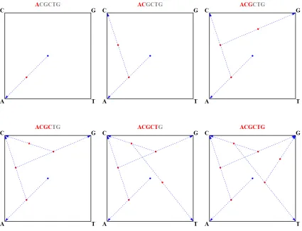
2.1 The Chaos Game Representation (CGR) of the DNA sequence ACGCTG. . . . 15
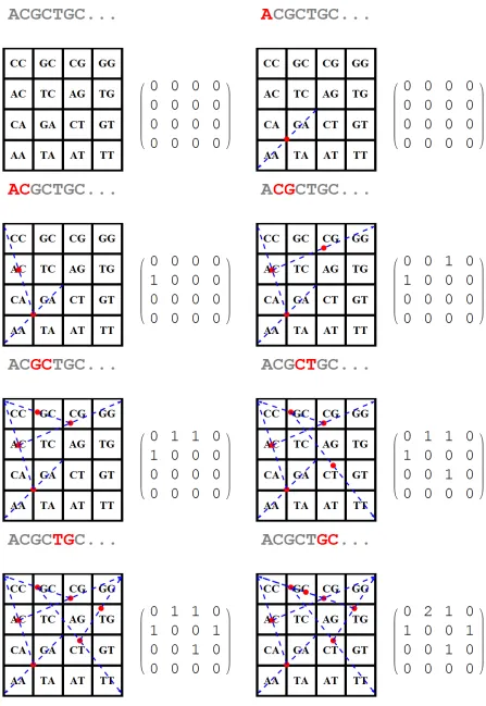
2.2 The Frequency Chaos Game Representation (FCGR) of the sequence ACGCTGC, fork= 2. The firstk−1 (here 2−1= 1) points do not alter the FCGR matrix. . 16
2.3 Chaos Game Representation (CGR) of nDNA fragments fromE. coli, S. cere-visiae,A. thaliana,P. falciparum,P. furiosusandH. sapiens. . . 18
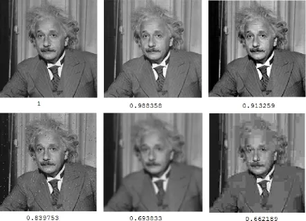
2.4 An example of computing SSIM similarity values for a set of 6 images. Upper left corner is the original image, hence similarity value is equal to 1. The rest of the images have various pixel values changed, blurred and distorted. The simi-larity between these images and the original image decreases. This example is
part of the examples demonstrated in https://ece.uwaterloo.ca/z70wang/research/ssim/ 22
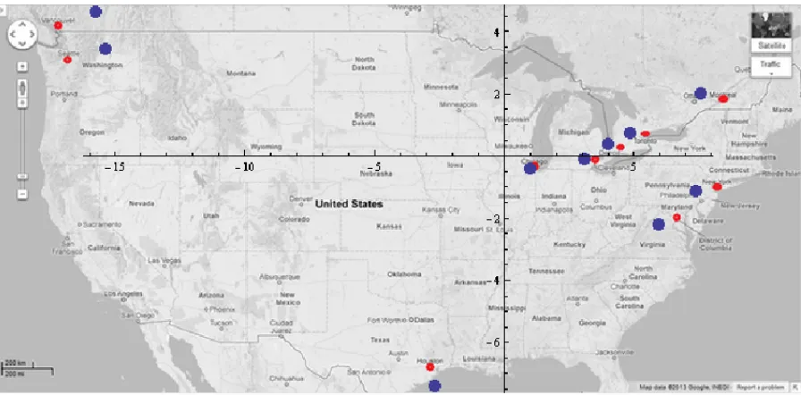
2.5 Multi-Dimensional Scaling (MDS) example. The red points are the real posi-tions of 10 big cities in North America. The blue points are the posiposi-tions of these cities as output of MDS. . . 24
3.1 CGR images for three DNA sequences. (a)Homo sapiens sapiens mtDNA, 16,569 bp; (b) Homo sapiens sapiens chromosome 11, beta-globin region, 73,308 bp; (c)Polypterus endlicherii (fish) mtDNA, 16,632 bp. Observe that chromosomal and mitochondrial DNA from the same species can display dif-ferent patterns, and also that mtDNA of different species may display visually similar patterns that are however sufficiently different as to be computationally distinguishable. . . 51
sented jawless vertebrates), with its five subphyla. (a) This Molecular Dis-tance Map comprises 1,791 mtDNA sequences, the average DSSIM disDis-tance is 0.8652, and the MDS Stress-1 is 0.12. Fish species bordering amphib-ians include fish with primitive pairs of lungs (Polypterus ornatipinnis#3125, Polypterus senegalus #2868), a fish who can breathe atmospheric air using a pair of lungs (Erpetoichthys calabaricus #2745), a toadfish (Porichtys myri-aster#2483), and all four represented lungfish (Protopterus aethiopicus#873, Lepidosiren paradoxa#2910,Neoceratodus forsteri #2957,Protopterus doloi #3119). Note that the question of whether species of the genusPolypterusare fish or amphibians has been discussed extensively for hundreds of years. Note also that gaps and spaces in clusters, in this and other maps, may be due to sampling bias. (b) Screenshot of the zoomed-in rectangular region outlined in Figure 3.2(a), obtained using the interactive web toolMoD Map[35]. . . 58
3.3 Molecular Distance Map of all represented species from (super)kingdom Protista and its orders. The total number of mtDNA sequences is 70, the av-erage DSSIM distance is 0.8288, and the MDSStress-1is 0.26. The sequence-point #1466 (red) is the unclassifiedHaemoproteussp. jb1.JA27, #1935 (grey) is Babesia bovis T2Bo, and #3173 (grey) is Theileria parva. The annotation shows that all these three species belong to the same taxonomic groups, Chro-malveolata, Alveolata, Apicomplexa, Aconoidasida, up to the order level. . . . 60
malia. The method successfully clusters taxonomic groups also at the Class level. Gaps and spaces in clusters, in this and other maps, may be due to sam-pling bias. A topic of further exploration would be to understand the cluster shapes and nature of the distribution of sequences in this figure. The total num-ber of mtDNA sequences is 790, the average DSSIM distance is 0.8139, and the MDSStress-1is 0.16. . . 61
3.5 Molecular Distance Map of class Amphibia and three of its orders.The to-tal number of mtDNA sequences is 112, the average DSSIM distance is 0.8445, and the MDSStress-1is 0.18. Note that the shape of the amphibian cluster and the (x,y)-coordinates of sequence-points are different here from those in Fig-ure 3.4. This is because MDS outputs a map that aims to preserve pairwise distances between points, but not necessarily their absolute coordinates. . . 62
3.6 Molecular Distance Map of order Primates and its suborders: Haplorrhini (anthropoids and tarsiers), and Strepsirrhini (lemurs, lorises, etc.).The to-tal number of mtDNA sequences is 62, the average DSSIM distance is 0.7733, and the MDS Stress-1 is 0.19. The outliers are Tarsius syrichta #1381, and Tarsius bancanus#2978, whose placement within the order Primates has been subject of debate for over a century. . . 64
3.7 Graph of the DSSIM distances between the CGR images ofHomo sapiens sapiensmtDNA and the CGR images of each of the 62 primate
mitochon-drial genomes (sorted by their distance from the human mtDNA).The dis-tances are in accordance with established phylogenetic trees: The species with the smallest DSSIM distances from Homo sapiens sapiensareHomo sapiens neanderthalensis,Home sapiens ssp. Denisova, followed by the chimp. . . 66
4.1 29 ×29 CGR images of 150 kbp genomic DNA sequences from H. sapiens, E. coli,S. cerevisiae,A. thaliana,P. falciparum, andP. furiosus. . . 83
genomic sequences spanning one complete chromosome from each of six or-ganisms, representing all kingdoms of life. The MoD Maps were obtained using DSSIM, descriptor, Euclidean, Manhattan, Pearson and approximated information distance, respectively. Each point corresponds to one 150 kbp ge-nomic sequence from: H. sapiens (blue), E. coli (green), S. cerevisiae (red), A. thaliana(turquoise),P. falciparum(magenta), andP. furiosus(orange). . . . 95
4.3 The first experiment: Three-dimensional Molecular Distance Maps of 150 kbp genomic sequences spanning one complete chromosome from each of six or-ganisms, representing all kingdoms of life. The MoD Maps were obtained using DSSIM, descriptor, Euclidean, Manhattan, Pearson and approximated information distance, respectively. Each point corresponds to one 150 kbp ge-nomic sequences from: H. sapiens(blue), E. coli (green), S. cerevisiae(red), A. thaliana(turquoise),P. falciparum(magenta), andP. furiosus(orange). . . . 96
4.4 The first experiment (150 kbp fragments spanning one complete chromosome per each of the six organisms): Histograms of pairwise intragenomic and in-tergenomic distances among the DNA sequences fromH. sapiensandA. thaliana.
. . . 98
4.5 The second experiment: Two-dimensional Molecular Distance Maps of DNA genomic sequences sampled from the entire genomes of all six organisms, ob-tained using DSSIM, descriptor, Euclidean, Manhattan, Pearson and approxi-mated information distance, respectively. The dataset consists of 10 randomly sampled fragments from each chromosome of multi-chromosome genomes, and all complete fragments from the genomes of E. coli and P. furiosus, for a total of 526 fragments. Each point corresponds to one such 150 kbp frag-ment from H. sapiens (blue), E. coli (green), S. cerevisiae (red), A. thaliana (turquoise),P. falciparum(magenta), andP. furiosus(orange). . . 101
nomic DNA sequences sampled from the genomes of all six chosen organisms, obtained using DSSIM, descriptor, Euclidean, Manhattan, Pearson and approx-imated information distance, respectively. The dataset consists of 10 randomly sampled fragments from each chromosome of multi-chromosome genomes, and all complete fragments from the genomes of E. coli and P. furiosus, for a total of 526 fragments. Each point corresponds to one such 150 kbp frag-ment from H. sapiens (blue), E. coli (green), S. cerevisiae (red), A. thaliana (turquoise),P. falciparum(magenta), andP. furiosus(orange). . . 102
4.7 The preview experiment: Two-dimensional Molecular Distance Maps of 150 kbp genomic DNA sequences, randomly sampled from each chromosome (10 frag-ments per chromosome) ofH. sapiens(blue),M. musculus(fuchsia) using the six distances. . . 111
4.8 The preview experiment: Three-dimensional Molecular Distance Maps of 150 kbp genomic DNA sequences, randomly sampled from each chromosome (10 frag-ments per chromosome) ofH. sapiens(blue),M. musculus(fuchsia) using the six distances. . . 112
5.1 3D Molecular Distance Map illustrating interrelationships among conventional nDNA signatures of 480 randomly sampled 150 kbp nuclear genomic frag-ments fromH. sapiens (blue) and 128 randomly sampled 150 kbp nuclear ge-nomic fragments fromD. melanogaster (orange). The accuracy of separation is 97.2%. . . 126
5.2 3D Molecular Distance Map illustrating interrelationships among conventional nDNA signatures of 480 randomly sampled nuclear genomic fragments from H. sapiens(blue) and 500 randomly sampled nuclear genomic fragments from P. troglodytes(red). All fragments are 150 kbp long, the accuracy of separation is 52.34%, and no separation plane could be found. . . 130
DNA signatures using nDNA and mtDNA, of 480 DNA fragments from H. sapiens(blue) and 500 DNA fragments fromP. troglodytes(red). The accuracy of separation is 100%. . . 133
5.4 3D Molecular Distance Map illustrating interrelationships among signatures of 380 DNA fragments fromB. napus (magenta) and 180 DNA fragments from B. oleracea (brown) using (a) conventional nDNA signatures, (b) composite DNA signatures using nDNA and mtDNA, (c) composite DNA signatures using nDNA and cpDNA, and (d) composite DNA signatures using nDNA, mtDNA, and cpDNA. The accuracy of separation is 63.03% for (a), and 100% for each of (b), (c), and (d). . . 134
5.5 3D Molecular Distance Map illustrating interrelationships among 480 compos-ite (respectively 480composite-assembled) DNA signatures, each using one nDNA fragment and the mtDNA genome fromH. sapiens, blue (resp. green); and 500 composite (resp. 500composite-assembled) DNA signatures, each using one nDNA fragment and the mtDNA genome from P. troglodytes, red (resp. turquoise); For the composite-assembled DNA signatures, the length of contigs was n = 100, while the number of contigs was 4,500 for each 150 kbp nDNA fragment, and 497 (resp. 496) for the human (resp. chimp) mtDNA genome. The accuracy of separation between theH. sapiensand the P. troglodytessequences was 58%, but the existence of a separation plane was verified. . . 143
5.6 Conventional nDNA signatures of 150 kbp sequences of the pivot organisms from Kingdom (a) Animalia, (b) Fungi, (c) Plantae, (d) Protista, (e) Bacteria, and (f) Archaea. . . 146
natures ofCapsicum annuum L, cultivarZunla-1(domesticated) shown in light green, and Capsicum annuum var. glabriusculum, cultivar Chiltepin (wild) shown in grey. . . 158
6.1 Molecular Distance Map of Phylum Vertebrata, consisting of 3,158 mtDNA sequences. Blue, cyan, green, red and yellow, represent fish, amphibia, reptiles, mammals and birds mtDNA genomes respectively. Enlarged version of left and right panel can be found in Figure 6.2 . . . 170 6.2 Enlarged version of left and rigth panel of MoDMaps3D. . . 171
4.1 Dataset for the first experiment: NCBI accession numbers of the complete chromosomes considered, in increasing order of their NCBI accession num-ber. . . 81
4.2 The first experiment: Organisms considered, total length of the chromosome (respectively genome), number of ignored letters “N”, and number of DNA fragments (sequences) obtained by splitting a single complete chromosome per organism into consecutive, non-overlapping, equal length (150 kbp) contiguous fragments. . . 81
4.3 The first experiment: Mean and standard deviation of distances between clus-tersCi−Cj fori, j= 1, ...,6. . . 99
4.4 The first experiment: Summary of quality measures for the performances of six distances (DSSIM, descriptor, Euclidean, Manhattan, Pearson, approximated information distance) on a dataset of 508 genomic DNA sequences spanning one complete chromosome for multi-chromosomes organisms and the com-plete genome otherwise, of one organism from each kingdom of life.Dαis the correlation to an idealized cluster, Aα the silhouette cluster accuracy, andOα
the relative overlap. Higher is better. . . 107
of six distances (DSSIM, descriptor, Euclidean, Manhattan, Pearson, approxi-mated information distance) on a dataset of 526 genomic DNA sequences sam-pled randomly (10 fragments per chromosome for multi-chromosome isms, and all fragments of the genome otherwise) from the genomes of organ-isms from each kingdom of life. Dα is the correlation to an idealized cluster,
Aα the silhouette cluster accuracy, andOαthe relative overlap. Higher is better. 108
4.6 The preview experiment: Summary of quality measures for the performances of six distances (DSSIM, descriptor, Euclidean, Manhattan, Pearson, approxi-mated information distance) on a dataset of 450 DNA sequences, sampled from the entire genome (10 fragments per chromosome) ofH. sapiensandM. mus-culus. Dαis the correlation to an idealized cluster,Aα is the silhouette cluster accuracy, andOαis the relative overlap. Higher is better. . . 110
5.1 Each subtable summarizes, for a given kingdom, the results of pairwise com-parisons between DNA signatures of fragments from a pivot organism (blue) and those from one other organism, at increasing levels of relatedness. The first two result columns indicate the outcome of the comparisons ofconventional
nDNA signatures, and the last two columns the comparisons of composite
DNA signatures. Green indicates that separation was achieved with AID, red
indicates that separation was not achieved with any of the six distances listed in Section 5.2, and yellow (Y/N) or Y* indicate results discussed in the text. The columns labelled Acc % indicate the accuracy of the separations listed imme-diately at their left: Acc > 85% was considered separation. A dash indicates that no sequenced data was available on NCBI/GenBank at the time of this submission. The corresponding 3D Molecular Distance Maps for each of the comparisons can be found in [58]. . . 127
fragment and its assembled DNA signatures, for various numbersrof contigs of the same length n: (A) distances to fully-assembled DNA signatures; (A0) theoretical upper bounds for (A); (B) distances to assembled DNA signatures; (C) same as (B), when tripling the number of contigs. (B0)through(C0) – Dis-tances between the conventional nDNA signature of a fragment and its assem-bled DNA signatures, using variable-length contigs taken from a normal distri-bution N(n, σ), with meannand variance σ = 40. The nDNA fragment used was fromH. sapiens, chromosome 21, fragment 20 (from position 2,850,001 to 3,000,000 after removing allNs in the original sequence). . . 136 5.3 Each subtable summarizes, for a given kingdom, the results of pairwise
com-parisons between DNA signatures of fragments from a pivot organism (blue) and those from one other organism, at increasing levels of relatedness. The first two result columns indicate the outcome of the comparisons ofconventional
nDNA signatures, and the last two columns the comparisons of composite
DNA signatures. Green indicates that separation was achieved with AID, red
indicates that separation was not achieved with any of the six distances listed in Section 5.2, and yellow (Y/N) or Y* indicate results discussed in the text. The columns labelled Acc % indicate the accuracy of the separations listed imme-diately at their left: Acc > 85% was considered separation. A dash indicates that no sequenced data was available on NCBI/GenBank at the time of this submission. The corresponding 3D Molecular Distance Maps for each of the comparisons can be found in [58]. . . 139
Introduction
Classic alignment-based methods (DNA barcoding [3], Klee diagrams [12], multiple sequence alignments [11]) have been used extensively for classification and identification of genomic sequences. Alignment-free methods provide an alternative for this task while having a few other advantages in terms of speed and applicability. After Karlinet al. suggested in [10] that k-mer frequencies can play the role of a genomic signature, there was an increasing interest
in the bioinformatics community to further explore and analyze genomic signatures. Jeffrey in [4, 5] introduced the use of Chaos Game Representation (CGR) of a DNA sequence giving a visual aspect to its structural properties, while later the study of CGRs was standardized by Deschavanneet al. in [2, 1].
Our goal is to find a general, universal method of classification based on the structural composition of genomic DNA. In this thesis, we continue the exploration of genomic signatures using CGRs and we extend results from other studies which were either qualitative or very limited in scope. In particular, we investigate whether or not CGR-based signatures can indeed act as genomic signatures. We also investigate the hypothesis that genomic signatures are preserved along a species’ genome. Finally, we test the discriminating power of CGRs for closely related species and we generalize genomic signatures by introducing two new types: “composite signature” and “assembled signature”.
Our proposed algorithm consists of three main components. Firstly, Chaos Game Repre-sentation (CGR) is being used to visualize and quantitatively express the syntactic structure of a DNA sequence. Secondly, a distance measure is employed to compute distances between CGRs of different DNA sequences. Notable distances being used in this thesis are Approxi-mated Information Distance (AID), Structural Similarity Index (SSIM) and Descriptors-based distance along with classical numerical distances such as Euclidean, Manhattan and Pearson distance. Finally, Multi-Dimensional Scaling (MDS) is used to reduce the dimensionality and efficiently embed the datapoints representing DNA sequences into a 2D or 3D Euclidean space, producing a Molecular Distance Map (MoDMap).
Our research findings are organized in the following way. Chapter 3 contains the article “Mapping the space of genomic signatures” [9] in which we perform an analysis of a mitochon-drial (mtDNA) dataset from the National Center for Biotechnology Information (NCBI) ex-ploring phylogenetic relationships and getting deeper insights on various unclassified spieces. Results of this extensive analysis confirm that the oligomer composition of full mtDNA se-quences can be a source of taxonomic information. Chapter 4 contains the article “An investi-gation into inter- and intragenomic variations of graphic genomic signatures” [7], in which we test the hypothesis of DNA genomic signatures being preserved along the genome of the same organism, while being dissimilar for DNA sequences originating from different organisms, at the kingdom level. We also assess six different distance measures and rank their performance based on statistical measures. Results suggest that several distances outperform the Euclidean distance, which has so far been almost exclusively used for such studies. Chapter 5 contains the article “Additive methods for genomic signatures” [8], in which we test the discriminating power of conventional CGR signatures of nuclear DNA sequences and we find, unexpectedly, that they do not suffice for distinguishing closely related species, for exampleH.sapiens and P.troglodytes. To overcome these limitations we extend the notion of genomic signature by
-ciently distinguish genomes even using less information than conventional genomic signatures. Finally, in Chapter 6 we present a web tool to explore, analyze and visualize genomic diversity on various DNA datasets [6]. The tool is written in JavaScript, is platform independent and can run in any modern web browser.
We conclude this thesis with Chapter 7, which contains a discussion about possible exten-sions of current work, including the search for a “representative” genomic signature of a species and haplogroup identification using human mitochondrial DNA data to track maternal lineage. Far more challenging tasks include backtracking paternal lineage in the Y chromosome and testing the ability of this method to distinguish between healthy and unhealthy populations with large scale mutations.
Bibliography
[1] P. Deschavanne, A. Giron, J. Vilain, C. Dufraigne, and B. Fertil. Genomic signature is preserved in short DNA fragments. Proceedings IEEE International Symposium on Bio-Informatics and Biomedical Engineering, 2000.
[2] P. Deschavanne, A. Giron, J. Vilain, G. Fagot, and B. Fertil. Genomic signature: char-acterization and classification of species assessed by chaos game representation of se-quences. Molecular Biology and Evolution, 16(10):1391–1399, 1999.
[3] Paul DN Hebert, Alina Cywinska, Shelley L Ball, et al. Biological identifications through DNA barcodes. Proceedings of the Royal Society of London. Series B: Biological Sci-ences, 270(1512):313–321, 2003.
[5] H. Jeffrey. Chaos game visualization of sequences. Computers&Graphics, 16(1):25–33, 1992.
[6] R. Karamichalis. Molecular Distance Maps 3D. https://github.com/rallis/ MoDMaps3D, 2016.
[7] R. Karamichalis, L. Kari, S. Konstantinidis, and S. Kopecki. An investigation into inter-and intragenomic variations of graphic genomic signatures.BMC Bioinformatics, 16:246, 2015.
[8] R. Karamichalis, L. Kari, S. Konstantinidis, S. Kopecki, and S. Solis-Reyes. Additive methods for genomic signatures. BMC Bioinformatics, 17:313, 2017.
[9] L. Kari, K. Hill, A. Sayem, R. Karamichalis, N. Bryans, K. Davis, and N. Dattani. Map-ping the space of genomic signatures. PloS ONE, 10(5):e0119815, 2015.
[10] S. Karlin and C. Burge. Dinucleotide relative abundance extremes: a genomic signature. Trends in Genetics, 11(7):283–290, 1995.
[11] Dan E Krane. Fundamental concepts of bioinformatics. Pearson Education India, 2003.
Genomic signatures
This chapter is organized in the following way. Firstly, an extensive literature review of re-search on genomic signatures is given, presenting a timeline of rere-search in this area. Various methods and tools that have been used for analyzing DNA sequences are presented. Secondly, the main methods employed throughout this thesis are presented. We give the definition of Chaos Game Representation (CGR) of a DNA sequence and its improved version, Frequency Chaos Game Representation (FCGR), together with an example. We also present various dis-tance measures to compute disdis-tances between CGRs. Finally, we present Multi-Dimensional Scaling (MDS) which is used for dimensionality reduction in the final stage of our proposed algorithm.
2.1
Literature review
Deoxyribonucleic Acid (DNA) is a molecule that encodes the genetic instructions used in the development and functioning of all known living organisms. As such, DNA has become a subject of both theoretical and applied studies for the last decades. DNA is a polymer of nucleotides. Nucleotides are the building blocks, or monomers of DNA. Each nucleotide is made of a phosphate, a deoxyribose sugar and a nitrogen base. The four different nucleotides of DNA are Adenine (A), Cytosine (C), Guanine (G), Thymine (T). DNA can be single stranded
or double stranded. In a double stranded DNA, the nucleotides are pairwise complementary, A is complementary to T, C is complementary to G. With this in mind, we can represent any DNA sequence as a string over a 4-letter alphabet consisting of letters A,C,G and T. In this thesis, we use various types of DNA, namely nuclear DNA (nDNA) which is the DNA located in the nucleus of eukaryotic cells, mitochondrial DNA (mtDNA) which is the DNA located in an organelle called mitochondrion and is responsible for energy production of the cell, chloroplast DNA (cpDNA) which is the DNA located in chloroplasts found mainly in land plants and algae, and plasmid DNA (pDNA) which is the DNA of plasmids mainly found in prokaryotes.
2.1.1
Graphical representations of DNA
After the first successful sequencing method reported by Fred Sanger in 1977 [149], various methods have been proposed to represent, explore and analyze DNA data. Initial studies pro-posed simple pictorial representations where each nucleotide is replaced with a specific symbol to represent it [121], or gap plots which visualize positional correlations and periodic patterns in a DNA sequence [102]. They were followed by representations of DNA sequences as ran-dom walks in 2D [121, 54, 124, 102, 118] where a DNA sequence is represented as a curve in a plane where the four possible moves, left/right and up/down, encode the four nucleotides. Enhanced versions of the 2D random walk were later proposed, namely the DB-curve which reduced degeneracy [185], and a modified version which eliminated degeneracy completely [192, 106]. Another approach, this time in 3D, introduced by Zhang et al. [204], was the Z-curve which was used to recognize coding protein genes in yeast [203], to build a database of Z-curves for more than 1000 genomes [202], and to build phylogenetic trees for 24 coro-noviruses [205]. A variation of Z-curve, the L-curve, was introduced in [110]. 4D curves based on Z-curves were also introduced in [162].
β-globin gene using both Euclidean and a custom Cosine distance in [108], and the use of the
Euclidean distance in 3-component vectors in [191]. Other studies perform analysis comput-ing similarity matrices uscomput-ing random walks, as for example for 8 codcomput-ing sequences of eukary-otes to reduce degeneracy of 2D curves [114], 50 β-globin genes and 127 protein kinase C enzymes to build “moment vectors” [193], 7 mammalian sequences using a custom distance called “Similar Factor” [75], ND5 proteins from 9 mammals [180], 35 mammalian mtDNA, 33 primate lentiviruses and 30 coronoviruses using Euclidean distance [194], and 35 mammals using whole mtDNA and Euclidean distance [76]. A Huffman-encoded version of 2D walk for 1-mers for the first exon ofβ-globin gene from 11 mammals was reported in [141].
Another approach to depict a DNA sequence is using a cell representation. Randic et al. was one of the first to use this method in order to overcome the problem of arbitrary assignment of the four nucleotides to symbols. His approach was based on the construction of a 12-component vector whose components are the leading eigenvalues of the L/L matrices (length/length) associated with the DNA sequence. This method was used for the first exon of
β-globin region of 11 mammals [145]. Various modifications along with tweaks and
optimiza-tions followed this study [112, 111, 190, 28, 107, 140, 142, 195] working mainly on small sets (less than 15) of exons ofβ-globin regions of mammals.
the first exon ofβ-globin gene for 10 mammals.
Detailed reviews about most of the graphical representations described above can be found in [147, 125].
2.1.2
k
-mer frequency-based methods
Many other tools have been used to perform statistical analysis and explore properties of DNA sequences in terms of k-mer composition. Philips et al. used Markov Chain of order 3 in nDNA of E.coli [135], and later the same method was used for nDNA of yeast [10]. Many studies that followed, suggested possible explanations for asymetrick-mer frequencies among which are that scarcity of CG in nDNA may reflect a requirement for mRNA stability [15], that scarcity of GATC in enterobacteriophages may be a result of the methyl-directed mismatch repair system [39], that scarcity of 4-mer and 6-mer palindromes in bacteria and bacterio-phages may be because of restriction/methylation regimes, recombination and transcription processes [91], that changes in 4-mer frequencies in nDNA of E.coli may have been altered by “Very Short Patch” repair process [16], that excess/scarcity of some 2,3,4-mers in gDNA, mtDNA and virusDNA may be due to DNA/RNA structure and regulatory mechanisms [25], that excess/scarcity of some 2,3,4-mers in phages, animal mtDNA, bacteria nDNA, vertebrate nDNA and chloroplasts cpDNA may be because of DNA structures (dinucleotide stacking energies, DNA curvature and superhelicity, nucleosome organization), context-dependent mu-tational events, methylation effects and processes of replication and repair [94, 90, 95] and that scarcity of 4,5,6-mer palindromes in bacterial and archaeal nDNA may be due to restriction enzymes [55].
along with Manhattan and/or Mahalanobis distance for analyzing DNA datasets such as 19 eukaryotes [93],E. coliand phage nDNA [94], nDNA from 51 prokaryotes and cpDNA from 11 plants [89], prokaryote nDNA, pDNA and mtDNA sequences [26], 504 bacterial pDNA and 230 nDNA [160], nDNA from 50 microbes [19], eukaryote nDNA [56], nDNA from 22 different species [83], and HIV-1 genomes from different years [131]. Dinucleotide Relative Abundance Profiles were later generalized to tetranucleotides (4-mers) and used to classify 27 microbial nDNA sequences [136], and to study inter-genomic distances among 636 prokaryotes [20].
As researchers started using frequency vectors of longer k-mers of lengths ranging from k = 4 to k = 8 the applications of this method became apparent. In the majority of these studies weighted or standardized Euclidean distance have been used, or slightly modified ver-sions of them [68, 182, 183]. Typical examples include building phylogenetic trees from nDNA sequences of 8 amniotes [152], 20 mammalian mtDNA sequences and 48 Hepatitis E genomes [32], and RAG1 genes from 46 vertebrates, 18S rRNA sequences from 93 plants and nDNA from 16 proteobacteria [27].
phylogenetic trees from intron sequences of 10 mammals. The same technique was used also in [181] for 142 dsDNA eukaryote viruses, in [154] for 36 nDNA sequences taken fromE. coli and someShigellaspecies, in [100] for 27 primate mtDNA and 13 Malvidae/plant nDNA, in [167] for 377H.pylorigenomes, and a webtool based on this was build in [74]. Using vectors ofk-mer occurrences one can also use the number ofk-word matches as a distance between two sequences. This distance which is usually denoted byD2is equivalent to the dot product of the k-mer occurrence vectors [113]. A variation of this, that considers up to tmismatches, is de-noted byDt2[24], while also some standardized and weighted versions exist [86, 146, 115, 14]. Many studies exist that study the statistical distribution properties [113, 24, 49, 48, 146, 84] and statistical power [173, 115, 157] of these distances. Such distances have been used for comparison of regulatory sequences [86] and for construction of phylogenetic trees for nDNA of 5 mammals and 13 tree species from NGS reads [157]. A few other studies used methods derived from k-mer vectors and usually mixed with custom distance measures. An example of such a method is the “discrimination measure” introduced in [46], which uses primitive discrimination substrings and was illustrated for 10 mammalian whole β-globin and 24 coro-naviruses. Another example is the “natural vectors” introduced in [35], which are based on normalized central moments and were tested with 51 influenza viruses, 99 human rhinovirus and 31 mammalian mtDNA. One more example is the “underlying approach” in [31], which is based on subword composition and tested with 54 H1N1 viruses, 18 prokaryote nDNA and 5Plasmodium nDNA. Finally, a last example is the entropy of Gamma distribution in [188], which is based on a k-mer voting model and was presented and tested with 30 mammalian mtDNA.
sequences [61], 442 proteins of 34 mammals [158], 21 plant chloroplasts together with several eubacteria, archaea, and eukaryote sequences [29], 139 prokaryotes [137], 16 archaea, 87 bac-teria, and 6 eukaryotes [138], 124 dsDNA viruses [51], 82 fungi [174] and 109 eukaryotes, 34 plant chloroplasts and 62 alpha-proteobacteria [201]. Successful applications ofk-mer vectors have also been reported in metagenomics for the classification of bacterial nDNA fragments from different species [148, 164]. In addition to this,k-mer vectors have been used along with Self-Organizing Maps (SOM), in order to classify hundreds of thousands of short prokaryote sequences into different phylogenetic groups in [3, 2, 120] and for various Drosophila genomes in [1]. Other applications ofk-mer frequencies include detection of horizontal transfers [79]. Efficient algorithms for parallel counting ofk-mers have been developed as well [119]. Logic Alignment Free (LAF) was also introduced and applied to bacterial genomes in [179]. LAF combines alignment-free techniques and rule-based classification to assign biological samples to their taxa, by searching for a minimal subset ofk-mers whose relative frequencies are used to build classification models as disjunctive-normal-form logic formulas. Finally, other studies transform the problem of classifying DNA sequences based onk-mer frequencies into classi-fying signals coming out of those. Initial studies analyzed small sets of genes [9], while later whole genome comparison using genomic signals was tested for eukaryotes in [155] and for prokaryotes in [151].
Many of the distances described for k-mer vectors have been compared and benchmarked in [184, 73, 72, 33, 34, 58, 80, 63], and detailed reviews of the literature can be found in [92, 169, 123, 21, 150, 156].
2.1.3
Other representations of DNA sequences
Markov models was used to build phylogenetic trees for genes ofE.coliandS.flexneriin [134], while a “weighted relative entropy” between Markov models was used to build phylogenies of 48 Hepatitis E viruses.
A few other studies focus on the multifractal analysis of the “measure representation” of DNA sequences, and were applied to bacterial nDNA in [197] and bacteria whole peptide transcript in [198]. Multifractal analysis has also been applied to exon and intron sequences [186] and to the human genome [53, 122]. Many statistical properties have been investigated in [159], and a fractal model to simulate phylogenetic relationships has been proposed in [199].
Some other studies perform Lempel-Ziv complexity-based analysis of DNA, where dis-tance measures are defined based on complexity measures of the sequences analyzed. Such methods were used to build phylogenies for 30 mammalian mtDNA in [127] using 4 distances based on Lempel-Ziv complexity, forCandida cytochrome band 18S rRNA for some medically relevant Fungi in [12], for 26 placental mammal mtDNA in [104], for the first exon ofβ-globin gene for 10 mammals together wth 12 H5N1 genomes in [114], for various protein datasets in [4], for 48 Hepatitis E viruses and 18 mammal mtDNA in [78], for 38 mammal mtDNA in [175] and for 16 rRNA ITS region of Galanthus plants in [11]. Various modifications of complexity-based distances have been defined also in [97, 47].
substitu-tions was derived and used for 27 primate mtDNA, 8Streptococcus agalactiaestrains and 12 DrosophilanDNA to compare the results against three other measures, while in [42] a faster version of [65] was reported and illustrated for 825 HIV-1 strains and 13E.colistrains. A sim-ilar estimator, this time for pairwise mismatches, was presented in [66] for 37D.melanogaster strains, and an improvement of it in [64] for 21Drosophilaspecies.
Various other representations combined with custom distances have been used in literature to analyze DNA datasets. A “Standardized Hasse” distance between Hasse matrices, based on partial ordering rules, was used for the first exon ofβ-globin genes from 8 mammals in [165]. Pattern-comparison based on linear predictive coding and its spectral distortion measure was used to classify genes fromE.coliandS.flexneriin [133]. The Euclidean distance between 16-dimensional vectors, called “base-base correlations”, were used for 48 Hepatitis E viruses and many prokaryote nDNA in [116] and for many coronoviruses in [117]. The Pearson distance between “average mutual information” profiles was used for classifying HIV-1 genomes by subtype in [13], and the Euclidean distance between information correlation matrices like [13] was tested for 218 dsDNA viruses in [52]. Finally, adjacency matrices of weighted digraphs were used with Euclidean, Cosine and Pearson distance for mtDNA genes of 12 primates in [139], the difference in free energy of nearest-neighbour interaction was presented in [206], Fourier transforms were proposed as a genomic signal processing distance and tested for 26 eukaryote 18S rRNA in [23], and “variable length local decoding” based on prefix codes was illustrated for 117 Hepatitis C viruses in [41].
2.2
Methods
2.2.1
Chaos Game Representation (CGR)
of DNA sequences, CGRs were initially used to analyze DNA sequences qualitatively [99, 69, 70, 60]. This led to the hypothesis expressed by Duttaet al. and Goldman, that CGR images represent no more information than second-order Markov chains [44, 57]. This hypothesis was later disproven by Almeidaet al.[6, 5] and others [176, 88]. Deschavanneet al.[38, 37] were the first to suggest that CGR is a good candidate for the role of genomic signature. The way a CGR of a DNA sequence is produced is as follows. Starting with a unit square with its four vertices labelled A, C, G, and T, clockwise starting from the bottom-left corner, we plot the very first point in the center of the square. We then read the sequence from left to rigth letter by letter, until the end of the sequence. For each letter being read, we plot a point in the middle of the segment connecting our currently drawn point and the vertex labelled with the letter we just read. An example demonstrating the procedure of plotting a CGR for a DNA sequence can be found in Figure 2.1. A set of various CGR plots can be found in Figure 2.3.
It turned out however, that representing a DNA sequence as a set of points being plotted in a unit square has its own limitations in terms of resolution and computer precision. This problem was later solved by Deschavanneet al. suggesting Frequency CGR (FCGR) as an extension of conventional CGR, where unit squares are in fact matrices of dimensions 2k× 2k, wherek is the resolution of FGCR. Each matrix entry represents the number of occurrences of a specific substring of lengthkin the original sequence. This way, FCGR can quantitatively express the structure and complexity of a DNA sequence as it contains the frequencies allk-mers of length up to a certain lengthk. An example of FCGR plot can be found in Figure 2.2.
used, some of which proving to perform better that those typically used. Pearson distance, along with a custom image distance have been used in [176] for 26 mtDNA sequences, DSSIM image distance has been used for over 3,000 mtDNA sequences in [88], and six different dis-tances have been used in [87] for nDNA fragments from organisms of all major kingdoms of life.
Other uses of CGRs have been reported in the literature as well. Deschavanne et al. in [40] used CGRs to classify functional families of proteins using reverse encoding of amino acids into nucleic sequences. An extension of CGR called Universal Sequence Map (USM) has been reported in [7, 8], which can be used for any size of alphabet. A three-dimensional CGR has been proposed in [163]. CGRs have also been used in studies to measure the degree of self-similarity within images (multifractal analysis) e.g., [196, 178, 50, 168, 122, 129, 128], to estimate sequence entropy [126, 170, 171], to detect horizontal transfers in prokaryotes in [43], to speed up local-alignment algorithms [85], to classify HPV genomes by genotype (together with Neural Networks) in [161], to propose a Recurrent Iterated Function Systems (RIFS) model tested in 50 eukaryotes in [200], to construct CGRs of multiple resolutions (in combination with Neural Networks) in [77] and to refactor foundational string problems using CGR-based algorithms in [172]. Protein sequence analysis using modified CGR and physico-chemical properties has been studied in [187].
2.2.2
Distance Measures
In this thesis, there are six distance measures being used and here we give the definition and a short description for each one of them. All of the distances are being applied to CGRs/FCGRs, that is, to 2k × 2k matrices with non-negative integers entries. Let
X = [xi j],Y = [yi j] with i, j = 1,2, . . .2k be matrices with non negative integer values, that is X,Y ∈
Z2
k×2k
≥0 . In order to compute the Euclidean, Manhattan and Pearson distances, we first convert the matrices X,Y ∈ Z2k×2k
≥0 into 1 ×4
k vectors. Now, for two vectors x,y ∈
Rn, their Euclidean distance
(a)E. coli (b) S. cerevisiae (c) A. thaliana
(d) P. falciparum (e) P. furiosus (f)H. sapiens
dE(x,y)=
v t n
X
i=1
(xi−yi)2,
dM(x,y)= n
X
i=1
|xi−yi|,
while their Pearson distancedP(x,y) is defined as
dP(x,y)=1−
σxy
σxσy
,
where
µx = 1 n
n
X
i=1
xi, σx =
v t
1 n−1
n
X
i=1
(xi−µx)2,
σxy= 1 n−1
n
X
i=1
(xi−µx)(yi−µy).
In general, σxy
σxσy ranges in the interval [−1,1], and as a result the Pearson distance ranges in the interval [0,2]. Euclidean and Manhattan distances are metrics (they are non-negative, symmet-ric and satisfy the triangle inequality). Pearson distance is not a metsymmet-ric.
Also, we define Approximated Information Distance dAID based on the Information Dis-tance defined in [105]. The Normalized Information DisDis-tance in [105] was based on the un-computable notion of Kolmogorov complexity. Using k-mers, the information distance be-tween two strings x,ywas defined as
d(x,y)= Nk(x|y)+Nk(y|x) Nk(xy)
with
Nk(x|y)= Nk(xy)−Nk(x)
whereNk(x) is the number of different, possibly overlapping,k-mers that occur inx.
previous distance, and is defined as
dAID(X,Y)=2−
f(X)+ f(Y) f(X+Y)
where f(X) = SumOfElements(Unitize(X)). By unitization of a matrixXwe mean that every non-zero entry becomes 1, while zeros remain 0. The reason behind this modification was that we wanted to avoid counting possible “extra”k-mers that are produced by the concatenation of two stringsxandy. This way, we are also guaranteed that
dAID(X,Y)=dAID(Y,X)
and
dAID(X,X)= 0
which are properties that were not present before. Approximated Information Distance is a metric.
The descriptor distance between two FCGRs X,Y ∈ Z2k×2k
≥0 aims to compare properties of the two given FCGRs of different scales. A descriptor is a vector characterized by the parametersmwhich is the size of the non-overlapping windows in which the FCGR is divided, rwhich is the number of intervals in the analysis, andrintervals which define the numbers of k-mer occurrences that are considered significant.
For givenm≤kandr, and intervals [a0,a1),[a1,a2),· · · ,[ar−1,ar) such thatS r−1
i=0[ai,ai+1)= [0,∞) and [ai,ai+1)∩[aj,aj+1) = ∅ ∀i, jwith i , j, we construct a descriptor in the follow-ing way. Firstly, we divide each of the two FCGR matrices X and Y into non-overlapping submatrices of size 2m×2m, resulting in 4k−m submatricesX
i j and Yi j withi, j = 1,· · · ,2k−m, which will be pairwise compared. Secondly, we compute for every Xi j a vector vecXi j =
1
vector vecXm,r and, using the same order of appending, we append all vectors vecYi j to form a new vector vecYm,r. For these parameter values ofm, r and the r chosen intervals, vecXm,r and vecYm,r are the “descriptors” of the FCGR matrices X and Y. Finally, we can combine descriptors vecXm,r(respectively vecYm,r) for several values of
mandrby appending them one after another, in the same order, to obtain the vector vecX(respectively vecY). Thedescriptor distancebetween the two FCGRs X andY is now defined as the Euclidean distance (and as a result is a metric) between the vectors vecXand vecY
dD(X,Y)= dE(vecX,vecY).
2.2.3
Multi-Dimensional Scaling (MDS)
Multi-Dimensional Scaling (MDS) is a statistical method [98] that has been used to visual-ize the degree of similarity between individual objects in a given dataset. MDS has been used extensively in various fields such as cognitive science, information science, psychomet-rics, marketing, ecology, social science, and other areas of study [22]. Applications of MDS to molecular biology studies can be found in [103] where it was used for the analysis of geo-graphic genetic distributions of some natural populations, in [67] where it was used to visualize distances among COI genes from various species, and in [71] where it was used to analyze and visualize relationships within collections of phylogenetic trees.
Given two pointsa,bin ther-dimensional Euclidean space we can directly compute their Euclidean distance as d(a,b) = pPri=1(ai −bi)2. MDS tries to solve the inverse problem. Given all the pairwise distancesdi j (i, j = 1,· · · ,n) betweenn objects, it tries to determine a set of vectors (that is, a set of points in ther-dimensional space) that have these distances as their distances. MDS finds a set of points in ther-dimensional Euclidean space such that the Euclidean distance between two objects is similar to the distances between the corresponding objects in the input distance matrixdi j.
More precisely, classical MDS, receives as input an n×ndistance matrix (∆(i, j))1≤i,j≤nof the pairwise distances between any two items in the set. MDS will returnnpointsp1,p2, . . . ,pn ∈
Rr such that d(i, j) = ||pi− pj|| ≈ f(∆(i, j)) for alli, j ∈ {1, . . . ,n}whered(i, j) is the spatial distance between the points pi and pj, and f is a function linear in∆(i, j). The value ofrcan be at mostn−1, while in most of the cases the value of eitherr= 2 orr= 3 is used to produce a visualization in 2D or 3D space, respectively.
points, approximate fairly well the topology of the red points. Some misplacement of points is expected because of measurement errors, mainly because roads connecting cities are not straight lines and because the Earth is not flat.
Bibliography
[1] T. Abe, Y. Hamano, and T. Ikemura. Visualization of genome signatures of eukaryote genomes by batch-learning self-organizing map with a special emphasis on drosophila genomes. BioMed Research International, 2014, 2014.
[2] T. Abe, H. Sugawara, S. Kanaya, and T. Ikemura. A novel bioinformatics tool for phy-logenetic classification of genomic sequence fragments derived from mixed genomes of uncultured environmental microbes. Polar Research, 20:103–112, 2006.
[3] T. Abe, H. Sugawara, M. Kinouchi, S. Kanaya, and T. Ikemura. Novel phylogenetic studies of genomic sequence fragments derived from uncultured microbe mixtures in environmental and clinical samples. DNA Research, 12(5):281–290, 2005.
[4] A. Albayrak, H. Otu, and U. Sezerman. Clustering of protein families into functional subtypes using Relative Complexity Measure with reduced amino acid alphabets. BMC Bioinformatics, 11:428, 2010.
[5] J. Almeida. Sequence analysis by iterated maps, a review. Briefings in Bioinformatics, 15(3):369–375, 2014.
[6] J. Almeida, J. Carrio, A. Maretzek, P. Noble, and M. Fletcher. Analysis of genomic sequences by chaos game representation. Bioinformatics, 17(5):429–437, 2001.
[7] J. Almeida and S. Vinga. Universal sequence map (USM) of arbitrary discrete se-quences. BMC Bioinformatics, 3:6, 2002.
[8] J. Almeida and S. Vinga. Computing distribution of scale independent motifs in biolog-ical sequences. Algorithms for Molecular Biology, 1:18, 2006.
[10] J. Arnold, A. Cuticchia, D. Newsome, W. Jennings, and R. Ivarie. Mono- through hex-anucleotide composition of the sense strand of yeast DNA: a Markov chain analysis. Nucleic Acids Research, 16(14):7145–7158, 1988.
[11] Y. Bakıs¸, H. Otu, N. Tas¸c¸ı, C. Meydan, N. Bilgin, S. Y¨uzbas¸ıo˘glu, and O. Sezerman. Testing robustness of relative complexity measure method constructing robust phyloge-netic trees for Galanthus L. using the relative complexity measure.BMC Bioinformatics, 14(1):1–12, 2013.
[12] D. Bastola, H. Otu, S. Doukas, K. Sayood, S. Hinrichs, and P. Iwen. Utilization of the relative complexity measure to construct a phylogenetic tree for fungi. Mycological Research, 108(Pt 2):117–125, 2004.
[13] M. Bauer, S. Schuster, and K. Sayood. The average mutual information profile as a genomic signature. BMC Bioinformatics, 9:48, 2008.
[14] E. Behnam, M. Waterman, and A. Smith. A geometric interpretation for local alignment-free sequence comparison. Journal of Computational Biology, 20(7):471–485, 2013.
[15] E. Beutler, T. Gelbart, J. Han, J. Koziol, and B. Beutler. Evolution of the genome and the genetic code: selection at the dinucleotide level by methylation and polyribonucleotide cleavage. Proceedings of the National Academy of Sciences of the United States of America, 86(1):192–196, 1989.
[16] A. Bhagwat and M. McClelland. DNA mismatch correction by very short patch repair may have altered the abundance of oligonucleotides in theE. coligenome.Nucleic Acids Research, 20(7):1663–1668, 1992.
[18] B. Blaisdell. Effectiveness of measures requiring and not requiring prior sequence align-ment for estimating the dissimilarity of natural sequences. Journal of Molecular Evolu-tion, 29(6):526–537, 1989.
[19] J. Bohlin. Genomic signatures in microbes – properties and applications. The Scientifc World Journal, 11:715–725, 2011.
[20] J. Bohlin and E. Skjerve. Examination of genome homogeneity in prokaryotes using genomic signatures. PLoS ONE, 4(12), 2009.
[21] O. Bonham-Carter, J. Steele, and D. Bastola. Alignment-free genetic sequence compar-isons: a review of recent approaches by word analysis.Briefings in Bioinformatics, page bbt052, 2013.
[22] I. Borg and P. Groenen. Modern Multidimensional Scaling: Theory and Applications. Springer, 2nd edition, 2010.
[23] E. Borrayo, E. Mendizabal-Ruiz, H. V´elez-P´erez, R. Romo-V´azquez, A. Mendizabal, and J. Morales. Genomic signal processing methods for computation of alignment-free distances from DNA sequences. PLoS ONE, 9(11), 2014.
[24] C. Burden, S. Forˆet, and S. Wilson. k-Word matches: an alignment-free sequence com-parison method. Supplementary Conference Proceedings PRIB 2008, pages 235–238, 2008.
[25] C. Burge, A. Campbell, and S. Karlin. Over- and under-representation of short oligonu-cleotides in DNA sequences. Proceedings of the National Academy of Sciences of the United States of America, 89(4):1358–1362, 1992.
[27] C. Chapus, C. Dufraigne, S. Edwards, A. Giron, B. Fertil, and P. Deschavanne. Explo-ration of phylogenetic data using a global sequence analysis method.BMC Evolutionary Biology, 5(1):1–18, 2005.
[28] R. Chi and K. Ding. Novel 4D numerical representation of DNA sequences. Chemical Physics Letters, 407(1-3):63–67, 2005.
[29] K. Chu, J. Qi, Z.-G. Yu, and V. Anh. Origin and phylogeny of chloroplasts revealed by a simple correlation analysis of complete genomes. Molecular Biology and Evolution, 21(1):200–206, 2004.
[30] G. Churchill. Hidden Markov chains and the analysis of genome structure. Computers
&Chemistry, 16(2):107–115, 1992.
[31] M. Comin and D. Verzotto. Alignment-free phylogeny of whole genomes using under-lying subwords. Algorithms for Molecular Biology : AMB, 7(1):34, 2012.
[32] Q. Dai, X. Liu, Y. Yao, and F. Zhao. Numerical characteristics of word frequencies and their application to dissimilarity measure for sequence comparison. Journal of Theoret-ical Biology, 276(1):174–180, 2011.
[33] Q. Dai and T. Wang. Comparison study on k-word statistical measures for protein: from sequence to ’sequence space’. BMC Bioinformatics, 9:394, 2008.
[34] Q. Dai, Y. Yang, and T. Wang. Markov model plus k-word distributions: A syn-ergy that produces novel statistical measures for sequence comparison. Bioinformatics, 24(20):2296–2302, 2008.
[36] P. Deschavanne, M. DuBow, and C. Regeard. The use of genomic signature distance between bacteriophages and their hosts displays evolutionary relationships and phage growth cycle determination. Virology Journal, 7:163, 2010.
[37] P. Deschavanne, A. Giron, J. Vilain, C. Dufraigne, and B. Fertil. Genomic signature is preserved in short DNA fragments. Proceedings IEEE International Symposium on Bio-Informatics and Biomedical Engineering, pages 161–167, 2000.
[38] P. Deschavanne, A. Giron, J. Vilain, G. Fagot, and B. Fertil. Genomic signature: char-acterization and classification of species assessed by chaos game representation of se-quences. Molecular Biology and Evolution, 16(10):1391–1399, 1999.
[39] P. Deschavanne and M. Radman. Counterselection of GATC sequences in enterobacte-riophages by the components of the methyl-directed mismatch repair system. Journal of Molecular Evolution, 33(2):125–132, 1991.
[40] P. Deschavanne and P. Tuffery. Exploring an alignment free approach for protein classi-fication and structural class prediction. Biochimie, 90(4):615–625, 2008.
[41] G. Didier, E. Corel, I. Laprevotte, A. Grossmann, and C. Land`es-Devauchelle. Variable length local decoding and alignment-free sequence comparison. Theoretical Computer Science, 462:1–11, 2012.
[42] M. Domazet-Loˇso Mirjana and B. Haubold. Efficient estimation of pairwise distances between genomes. Bioinformatics, 25(24):3221–3227, 2009.
[43] C. Dufraigne, B. Fertil, S. Lespinats, A. Giron, and P. Deschavanne. Detection and characterization of horizontal transfers in prokaryotes using genomic signature.Nucleic Acids Research, 33(1):e6, 2005.
algorithms for nucleotide sequence analysis.Journal of Molecular Biology, 228(3):715– 719, 1992.
[45] S. Edwards, B. Fertil, A. Giron, and P. Deschavanne. A genomic schism in birds revealed by phylogenetic analysis of DNA strings. Systematic Biology, 51(4):599–613, 2002.
[46] J. Feng, Y. Hu, P. Wan, A. Zhang, and W. Zhao. New method for comparing DNA primary sequences based on a discrimination measure. Journal of Theoretical Biology, 266(4):703–707, 2010.
[47] P. Ferragina, R. Giancarlo, V. Greco, G. Manzini, and G. Valiente. Compression-based classification of biological sequences and structures via the Universal Similarity Metric: experimental assessment. BMC Bioinformatics, 8:252, 2007.
[48] S. Forˆet, S. Wilson, and C. Burden. Characterizing the D2 statistic: word matches in biological sequences. Statistical Applications in Genetics and Molecular Biology, 8(1):Article 43, 2009.
[49] S. Forˆet, S. Wilson, and C. Burden. Empirical distribution of k-word matches in biolog-ical sequences. Pattern Recognition, 42(4):539–548, 2009.
[50] W. Fu, Y. Wang, and D. Lu. Multifractal analysis of genomes sequences’ CGR graph. Journal of Biomedical Engineering, 24(3):522–525, 2007.
[51] L. Gao and J. Qi. Whole genome molecular phylogeny of large dsDNA viruses using composition vector method. BMC Evolutionary Biology, 7(1):41, 2007.
[52] Y. Gao and L. Luo. Genome-based phylogeny of dsDNA viruses by a novel alignment-free method. Gene, 492(1):309–314, 2012.
[54] M. Gates. A simple way to look at DNA. Journal of Theoretical Biology, 119(3):319– 328, 1986.
[55] M. Gelfand and E. Koonin. Avoidance of palindromic words in bacterial and ar-chaeal genomes: A close connection with restriction enzymes. Nucleic Acids Research, 25(12):2430–2439, 1997.
[56] A. Gentles and S. Karlin. Genome-scale compositional comparisons in eukaryotes. Genome Research, 11(4):540–546, 2001.
[57] N. Goldman. Nucleotide, dinucleotide and trinucleotide frequencies explain patterns observed in chaos game representations of DNA sequences. Nucleic Acids Research, 21(10):2487–2491, 1993.
[58] F. Guyon, C. Brochier-Armanet, and A. Gu´enoche. Comparison of alignment free string distances for complete genome phylogeny. Advances in Data Analysis and Classifica-tion, 3(2):95–108, 2009.
[59] F. Guyon and A. Gu´enoche. An evolutionary distance based on maximal unique matches. Communications in Statistics Theory and Methods, 39(3):385–397, 2010.
[60] B. Hao, H. Lee, and S. Zhang. Fractals related to long DNA sequences and complete genomes. Chaos, Solitons and Fractals, 11(6):825–836, 2000.
[61] B. Hao and J. Qi. Prokaryote phylogeny without sequence alignment: from avoidance signature to composition distance. Journal of Bioinformatics and Computational Biol-ogy, 02(01):1–19, 2004.
[62] K. Hatje and M. Kollmar. A phylogenetic analysis of the brassicales clade based on an alignment-free sequence comparison method. Frontiers in Plant Science, 3, 2012.
[64] B. Haubold and P. Pfaffelhuber. Alignment-free population genomics: An efficient esti-mator of sequence diversity. G3: Genes—Genomes—Genetics, 2(8):883–889, 2012.
[65] B. Haubold, P. Pfaffelhuber, M. Domazet-Loso, and T. Wiehe. Estimating mutation distances from unaligned genomes. Journal of Computational Biology, 16(10):1487– 1500, 2009.
[66] B. Haubold, F. Reed, and P. Pfaffelhuber. Alignment-free estimation of nucleotide di-versity. Bioinformatics, 27(4):449–455, 2011.
[67] P. Hebert, A. Cywinska, S. Ball, and J. deWaard. Biological identifications through DNA barcodes. Proceedings of the Royal Society of London B: Biological Sciences, 270(1512):313–321, 2003.
[68] W. Hide, J. Burke, and D. Davison. Biological evaluation of D2, an algorithm for high-performance sequence comparison. Journal of Computational Biology, 1(3):199–215, 1994.
[69] K. Hill, N. Schisler, and S. Singh. Chaos game representation of coding regions of human globin genes and alcohol dehydrogenase genes of phylogenetically divergent species. Journal of Molecular Evolution, 35(3):261–269, 1992.
[70] K. Hill and S. Singh. The evolution of species-type specificity in the global DNA se-quence organization of mitochondrial genomes. Genome, 40(3):342–356, 1997.
[71] D. Hillis, T. Heath, and K. John. Analysis and visualization of tree space. Systematic Biology, 54(3):471–482, 2005.
[72] M. H¨ohl and M. Ragan. Is multiple-sequence alignment required for accurate inference of phylogeny? Systematic Biology, 56(2):206–221, 2007.
[74] S. Horwege, S. Lindner, M. Boden, K. Hatje, M. Kollmar, C. Leimeister, and B. Mor-genstern. Spaced words and kmacs: Fast alignment-free sequence comparison based on inexact word matches. Nucleic Acids Research, 42(W1), 2014.
[75] G. Huang, B. Liao, Y. Li, and Y. Yu. Similarity studies of DNA sequences based on a new 2D graphical representation. Biophysical Chemistry, 143(1-2):55–59, 2009.
[76] G. Huang, H. Zhou, Y. Li, and L. Xu. Alignment-free comparison of genome sequences by a new numerical characterization. Journal of Theoretical Biology, 281(1):107–112, 2011.
[77] X. Huang, D.-S. Huang, H.-Q. Wang, and X.-M. Zhao. Representation of DNA se-quences with multiple resolutions and BP neural network based classification. InNeural Networks, 2004, volume 2, pages 1185–1189. IEEE, 2004.
[78] Y. Huang, L. Yang, and T. Wang. Phylogenetic analysis of DNA sequences based on the generalized pseudo-amino acid composition. Journal of Theoretical Biology, 269(1):217–223, 2011.
[79] K. Jaron, J. Moravec, and N. Mart´ınkov´a. Sighunt: horizontal gene transfer finder opti-mized for eukaryotic genomes. Bioinformatics, 30(8):1081–1086, 2014.
[80] R. Jayalakshmi, R. Natarajan, M. Vivekanandan, and G. Natarajan. Alignment-free sequence comparison using N-dimensional similarity space. Current Computer-Aided Drug Design, 6(4):290–296, 2010.
[81] H. Jeffrey. Chaos game representation of gene structure. Nucleic Acids Research, 18(8):2163–2170, 1990.
[83] R. Jernigan and R. Baran. Pervasive properties of the genomic signature. BMC Ge-nomics, 3(1):23, 2002.
[84] J. Jing, C. Burden, S. Forˆet, and S. Wilson. Statistical considerations underpinning an alignment-free sequence comparison method. Journal of the Korean Statistical Society, 39(3):325–335, 2010.
[85] J. Joseph and R. Sasikumar. Chaos game representation for comparison of whole genomes. BMC Bioinformatics, 7:243, 2006.
[86] M. Kantorovitz, G. Robinson, and S. Sinha. A statistical method for alignment-free comparison of regulatory sequences. Bioinformatics, 23(13):i249–i255, 2007.
[87] R. Karamichalis, L. Kari, S. Konstantinidis, and S. Kopecki. An investigation into inter- and intragenomic variations of graphic genomic signatures. BMC Bioinformat-ics, 16:246, 2015.
[88] L. Kari, K. Hill, A. Sayem, R. Karamichalis, N. Bryans, K. Davis, and N. Dattani. Mapping the space of genomic signatures. PloS ONE, 10(5):e0119815, 2015.
[89] S. Karlin. Global dinucleotide signatures and analysis of genomic heterogeneity. Cur-rent Opinion in Microbiology, 1(5):598–610, 1998.
[90] S. Karlin and C. Burge. Dinucleotide relative abundance extremes: a genomic signature. Trends in Genetics, 11(7):283–290, 1995.
[91] S. Karlin, C. Burge, and A. Campbell. Statistical analyses of counts and distributions of restriction sites in DNA sequences. Nucleic Acids Research, 20(6):1363–1370, 1992.
[93] S. Karlin and I. Ladunga. Comparisons of eukaryotic genomic sequences. Proceedings of the National Academy of Sciences of the United States of America, 91(26):12832–
12836, 1994.
[94] S. Karlin, I. Ladunga, and B. Blaisdell. Heterogeneity of genomes: measures and val-ues. Proceedings of the National Academy of Sciences of the United States of America, 91(26):12837–12841, 1994.
[95] S. Karlin, J. Mrzek, and A. Campbell. Compositional biases of bacterial genomes and evolutionary implications. Journal of Bacteriology, 179(12):3899–3913, 1997.
[96] P. Kolekar, M. Kale, and U. Kulkarni-Kale. Alignment-free distance measure based on return time distribution for sequence analysis: Applications to clustering, molecu-lar phylogeny and subtyping. Molecular Phylogenetics and Evolution, 65(2):510–522, 2012.
[97] N. Krasnogor and D. Pelta. Measuring the similarity of protein structures by means of the Universal Similarity Metric. Bioinformatics, 20(7):1015–1021, 2004.
[98] J. Kruskal. Multidimensional scaling by optimizing goodness of fit to a nonmetric hy-pothesis. Psychometrika, 29(1):1–27, 1964.
[99] B. Kumar, R. Alok, B. Sk, and D. Jayant. Genome analysis: A new approach for visu-alization of sequence organization in genomes. Journal of Biosciences, 17(4):395–411, 1992.
[100] C. Leimeister, M. Boden, S. Horwege, S. Lindner, and B. Morgenstern. Fast alignment-free sequence comparison using spaced-word frequencies. Bioinformatics, 30(14):1991–1999, 2014.