Three Experiments on Complex Fluids

(1)

Western University Western University

Scholarship@Western

Electronic Thesis and Dissertation Repository

12-13-2017 2:30 PM

Three Experiments on Complex Fluids

Yang Liu

The University of Western Ontario

Supervisor John R de Bruyn

The University of Western Ontario Graduate Program in Physics

A thesis submitted in partial fulfillment of the requirements for the degree in Doctor of Philosophy

Follow this and additional works at: https://ir.lib.uwo.ca/etd

Part of the Fluid Dynamics Commons

Recommended Citation Recommended Citation

Liu, Yang, "Three Experiments on Complex Fluids" (2017). Electronic Thesis and Dissertation Repository. 5118.

https://ir.lib.uwo.ca/etd/5118

This Dissertation/Thesis is brought to you for free and open access by Scholarship@Western. It has been accepted for inclusion in Electronic Thesis and Dissertation Repository by an authorized administrator of

(2)

Abstract

The behaviour of complex fluids is fundamentally interesting and important in many

ap-plications. This thesis reports on three experiments on the thermal and rheological behaviour

of complex fluids. The first is a study of the rheological properties of and heat transport in a

saline solution of hydroxyethyl cellulose. This material has been used as a tissue phantom in

testing the behavior of medical devices in MRI scanners. We find it behaves as a typical

entan-gled polymer, and flows in response to local heating, such as could occur due to eddy-current

heating of metallic devices in an MR scanner. We use laboratory experiments and numerical

simulations to determine the convective and conductive contributions to the heat transport in a

simple model of this system. Our results indicate that convective heat transport is of the same

order of magnitude as conductive transport under conditions typical of MRI device tests. The

second project is an investigation of the start-up flow and yielding of a simple yield-stress fluid

(Carbopol 940) in a vertical pipe. The Carbopol was displaced from below by an immiscible

Newtonian liquid (Fluorinert FC-40) injected at a constant, controlled rate. Rough and

smooth-walled pipes were used to study the eﬀects of wall boundary conditions. In the rough-walled

pipe, the yielding involved a long transient with several steps: elastic deformation, the onset

of wall slip, yielding at the wall, and finally a steady-state plug flow that is well-described

by the predictions of the Herschel-Bulkley model. In contrast, in the smooth-walled pipe, the

wall shear stress never exceeded the yield stress. In the third project, we study the flow of

Carbopol solutions confined to square microchannels with sides ranging from 500 down to 50

µm. In the larger channels, the measured velocity profiles agreed well with simulations based on the bulks-scale rheology of the Carbopol and the Herschel-Bulkley model. In contrast, in

microchannels with sides less than 150µm the velocity profiles could not be fitted by a model with a finite yield stress, but instead were described by a power-law model with zero yield

stress. We explain the vanishing of the yield stress in terms of the confinement of the

(3)

bopol’s microstructure by the microchannels.

Keywords: Rheology, complex fluids, yielding, yield stress, confinement

(4)

Co-Authorship Statement

The work in chapter 3 has been published as: Yang Liu, Cameron C. Hopkins, William

B. Handler, Blaine A. Chronik, John R. de Bruyn, Rheology and heat transport properties

of a hydroxyethyl cellulose-based MRI tissue phantom, Biomedical Physics & Engineering

Express, 3:045008, 2016. I did all the experiments and data analysis and wrote early drafts of

this paper. Cameron C. Hopkins performed the numerical simulations. William B. Handler and

Blaine A. Chronik provided the HEC solutions and the expertise on MRI applications. All the

authors provided editorial comments on this paper. John R. de Bruyn supervised the project.

The work in chapter 4 has been submitted for publication: Yang Liu, John R. de Bruyn,

Start-up flow of a yield-stress fluid in a vertical pipe, Journal of Non-Newtonian Fluid

Me-chanics. I did all the experiments, simulations, and data analysis and was the primary author

of the paper. John R. de Bruyn supervised the project and provided editorial comments on the

paper.

The work in chapter 5 will be submitted for publication toJournal of Non-Newtonian Fluid

Mechanics. The authors include Yang Liu, Daniel Lorusso, David Holdworth, Tamie L.

Poep-ping, John R. de Bruyn. I designed the experiment, made the microchannels, and did all the

experiments, simulations, and data analysis, and was the primary author of the paper. Daniel

Lorusso and David Holdworth provided instruction and assistance in fabricating the channels.

Tamie L. Poepping provided equipment and expertise in the use of the channels and micro PIV.

John R. de Bruyn supervised the project and provided editorial comments on the paper.

(5)

Acknowledgments

I am highly indebted to my supervisor, Dr. John R. de Bruyn, for advising me with much

patience over the last five years. I learned how to do research the right way from John. None

of my work would have been possible without his support.

Special thanks go to Dr. Blaine A. Chronik and Dr. Tamie L. Poepping for cooperation and

collaboration in my research. Without their participation, I would not have finished this big

work.

Thanks also go to the Natural Sciences and Engineering Research Council of Canada and

the University of Western Ontario for funding this research. We are grateful to P. de Souza

Mendes for helpful conversations and to Ranjith Divigalpitiya of 3M Canada for providing the

Fluorinert.

My advisory committee, Dr. Richard A. Holt and Dr. Michael G. Cottam, provided helpful

advice at regular intervals throughout the project, and for this I’m grateful.

Here at the Department of Physics I worked with a number of fellow graduate students. I

wish to thank Cameron C. Hopkins who did some Comsol simulations for me and reviewed

the first draft of the introductory chapter of this thesis, and Nirosh Getangama and Nayeob Gi

who helped me to format this thesis using LATEX. Thanks also to former colleagues Grace

Ge, Maryam Mozaﬀari, and Masha Goiko who all contributed in many ways.

Brian Dalrymple and Frank Van Sas manufactured parts of the apparatus used in my

exper-iments. Tim Goldhawk and Todd Simpson assisted me in Nanofabrication Lab. Thanks also to

Henry Leparskas for computer support.

I especially want to thank Clara Buma, Jodi Guthrie, Brian Davis, Shailesh Nene and Phin

Perquin who always treated me with kindness.

Finally, I must give thanks to my family members, including my parents and other

rela-tives, who contributed so much to my education, career, and growth. Without their eﬀorts and

support, I would not have reached this far.

(6)

List of Figures

1.1 Diagram showing shear stress, strain, and shear rate in a layer of fluid between two

horizontal plates. The upper plate moves with a velocityv, while the lower plate is

fixed. . . 2

1.2 Left: Diagram of the Maxwell Model. The right graphs show the stress relaxation behaviour obtained by solving the model for ˙γ(t>0 s)=0 s−1andτ(t=0 s)=τ0Pa. . . 4

1.3 Left: Diagram of the Kelvin–Voigt Model. The right graph shows the strain creeping behaviour obtained by solving the model forτ(t<0 s)=0 Pa,τ(t≥0 s)=τ0Pa, andγ(t=0 s)=0. . . 5

1.4 Flow curves of diﬀerent types of fluids. . . 6

1.5 Flow curves of a thixotropic fluid measured with increasing steps in the shear rate and then decreasing steps. . . 11

1.6 The flow curve solved form>1 using Eq. (1.8). . . 13

2.1 The chemical formula of Hydroxyethyl cellulose (HEC). . . 26

2.2 The chemical formula of polyacrylic acid. . . 28

2.3 The microstructure of Carbopol. The dashed circles represent the swollen polymer blobs. . . 29

2.4 A schematic diagram of the cone-and-plate measuring tool of the shear rheometer. Ω is the angular velocity of the rotating cone.θ0is the cone angle. . . 30

2.5 Two successive video frames used for PIV analysis. The bright points are small parti-cles suspended in the experimental fluid and illuminated by a light source. The squares in the frames are interrogation windows. . . 32

(11)

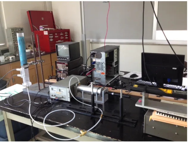
2.6 The overall set-up of the experiments in Chap. 4. . . 35

2.7 Some components of the overall apparatus shown in Fig. 2.6. . . 35

2.8 Left: GPIB-USB-HS (IEEE 488) used to connect voltmeters to the computer. Right:

PCI-1407 (IMAQ) hardware used to connect the camera to the computer. . . 37

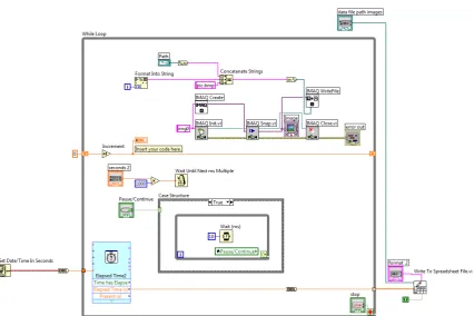
2.9 The LabVIEW block diagram code controlling the camera in the experiments

de-scribed in Chaps. 3 and 4. . . 38

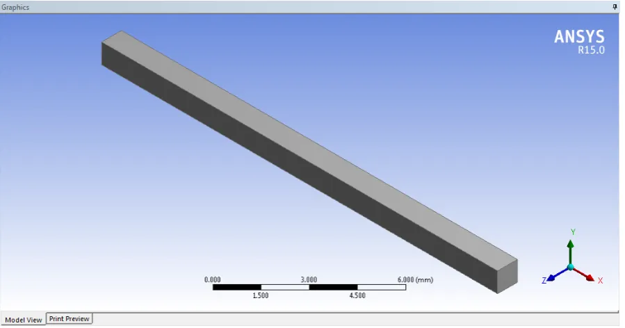
2.10 The computational domain used to simulate a channel in Chap. 5. . . 40

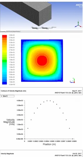
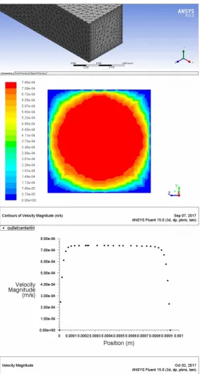
2.11 The results of a simulation for water flowing in the channel shown in Fig. 2.10. Top:

the computational mesh used in the simulations. Middle: the simulated velocity map

at the outlet of the channel. Bottom: the simulated velocity profile on the mid-height

line at the outlet of the channel. . . 41

2.12 The results of a simulation for Carbopol in the channel shown in Fig. 2.10. Top: the

computational mesh used in the simulations. Middle: the simulated velocity map at

the outlet of the channel. Bottom: the simulated velocity profile on the mid-height line

at the outlet of the channel. . . 42

3.1 The experimental set-up used to measure convective heat transport in fluids.

A tank contains the fluid of interest, which is seeded with small flow

visual-ization particles. The tank is 30.5±0.1 cm in length, 21.2±0.1 cm in height,

and 15.5±0.1 cm in width into the page. A heater is mounted at the left-hand

edge of the tank, and the temperature measured at four locations with optical

temperature probes. The visualization particles are illuminated by a laser sheet

coming in from the right-hand side of the diagram, and their motion is recorded

by a video camera looking into the page. The dotted rectangle indicates the

re-gion imaged by the camera. The origin of thex-ycoordinate system shown is

at the bottom left corner of the tank. . . 49

(12)

3.2 (a) The shear stressσas a function of shear rate ˙γof the HEC-saline solution at 25◦C. The waiting time at each value of ˙γwas 1 min. (b) Viscosityηobtained form the data plotted in (a). The dashed lines are fits to the Cross model, Eq.

(3.2). The open circles are for fresh HEC, while the filled circles are for the

aged solution. The inset shows the viscosity at a ˙γ = 1 s−1 _{measured with} diﬀerent values of the waiting time. . . 52

3.3 The zero-shear-rate viscosityη0for both fresh and aged HEC solutions plotted as a function of temperature. The open and filled circles are data for the fresh

and aged HEC solutions, respectively. The dashed lines are fits to Eq. (3.3), as

discussed in the text. . . 52

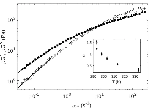
3.4 Elastic and viscous moduli of the fresh HEC-saline solution, scaled to a

tem-perature of 25◦C using time-temperature superposition. The diﬀerent symbols

indicate data recorded at diﬀerent temperatures: ⃝: 20◦C, : 25◦C, ▽: 30◦C,

△: 40◦C,⋄: 60◦C. Solid symbols areG′′ and open symbols areG′. The dashed

lines are power-law fits to the lowest-frequency data. The inset shows the

fre-quency scaling factor α for fresh (open symbols) and aged (solid symbols) HEC-saline solution. . . 54

3.5 The velocity field measured in an experiment using water. The field of view

is at the top left of the fluid, in a vertical plane through the center of the tank,

as discussed in the text. The edge of the heater is at x = 0; the bottom of the

tank is ay y = 0, and the free surface of the fluid is at the top of the image.

The tip of temperature probe 1 is close to the heater, and the dotted line shows

the approximate position of temperature probe 2. The temperature diﬀerence

between these two probes was 4.2 K. The length of the scale bar at the top left

corresponds to a velocity of 0.05 cm/s. . . 55

(13)

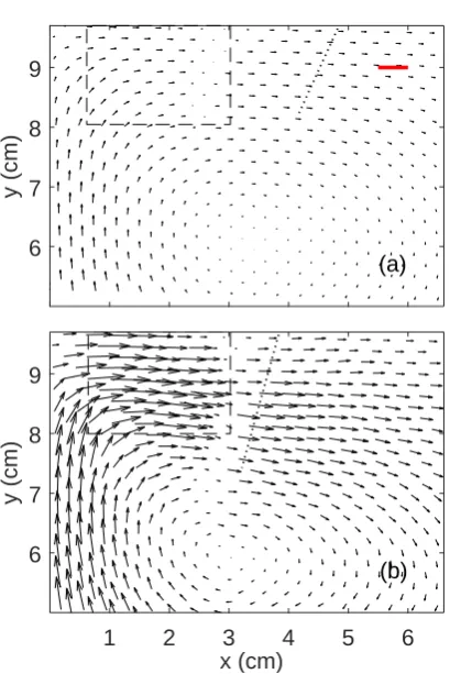
3.6 The velocity field in experiments on the HEC solution. (a) shows the velocity

field when the temperature diﬀerence between probes 1 and 2 was 10.8 K; (b)

is for a temperature diﬀerence of 49 K. The field of view is at the top left of the

fluid, in a vertical plane through the center of the tank, as discussed in the text.

The edge of the heater is atx = 0; the bottom of the tank is ayy = 0, and the

free surface of the fluid is at the top of the image. The tip of temperature probe

1 is close to the heater, and the dotted line shows the approximate position

of temperature probe 2. The length of the scale bar at the top right of (a)

corresponds to a velocity of 3×10−3cm/s. . . 58

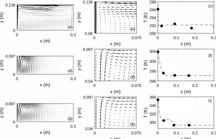
3.7 Simulations of the flow and temperature fields for the three experiments

de-scribed in the text. (a)-(c): Water, T1 = 295.9 K; (d)-(f): HEC solution, T1 = 304.7 K, (g)-(i): HEC solution, T1 = 352.8 K. The left-hand column shows the velocity field in the entire simulated domain, which models the tank

used in the experiments. The center column shows the velocity field in the

upper left corner of the domain. This corresponds to the region in which the

velocity was measured experimentally, as shown in Figs. 3.5 and 3.6. The

right-hand column shows the temperatures measured at the four probes as solid

circles, and the simulated temperature at approximately the same depth as a

dashed line. . . 59

4.1 The shear stressτas a function of shear rate ˙γ of 0.13 wt% Carbopol containing 0.6

vol% glass beads. Symbols are the measured data, and the dashed line is a fit to the

Herschel-Bulkley model, as described in the text. . . 70

4.2 A schematic diagram of the experimental apparatus. P1 and P2 are pressure gauges.

The solid horizontal line near the bottom of the pipe is the interface between the

Car-bopol and Fluorinert. The area between the dotted lines is the region used for flow

visualization. . . 72

(14)

4.3 Data from an experiment using 0.18 wt% Carbopol in the rough-walled pipe with a

very slow displacement rate,Ql = 5.02×10−8 m3/s. (a)P1, the pressure in the

Car-bopol. The dashed lines are linear fits to P1(t) at early (160-200 s) and late times

(300-400 s). The time at which the two fits intersect ist∗. (b)τw, the wall shear stress,

calculated from Eq. (4.1). The black circle isτ∗_w, the wall shear stress att∗. The dashed

line is the yield stress measured with the rheometer. The three time intervals discussed

in the text and in Fig. 4.4 are shown by the grey rectangles. The uncertainty ofτwis

approximately the size of the symbols. . . 74

4.4 The flow velocity v(r) corrected for the slip velocity vs for the same experiment as

in Fig. 4.3. The r axis spans the full diameter of the pipe. The dashed line is the

steady-state velocity profile predicted by the HB model. . . 75

4.5 Additional results for the experiment shown in Fig. 4.3. (a)Q, the volumetric flow

rate. (b)|γw˙ |, the absolute value of the wall shear rate. (c)vs, the slip velocity. . . 75

4.6 Data from an experiment using 0.18 wt% Carbopol in the rough-walled pipe with a

displacement rate ofQl = 3.41×10−7 m3/s. (a) τw, the wall shear stress. The dark

circle isτ∗_w, and the dashed line is the yield stress. The rectangles indicate the three

time intervals referred to in Fig. 4.7. The uncertainty ofτwis approximately the size

of the symbols. (b)vs, the slip velocity. (c) |γw˙ |, the absolute value of the wall shear

rate. . . 76

4.7 Velocity profiles for the same experiment as in Fig. 4.6. The dashed line is the velocity

profile predicted by the HB model. . . 77

4.8 Results of two experiments with 0.18 wt% Carbopol in the smooth-walled pipe. (a),

(b), and (c) are from an experiment with a low displacement rate, Ql = 5.02×10−8

m3/s. (a) τw, the wall shear stress. The black circle is τ∗_w. The two time intervals

discussed in the text are shown by rectangles. (b) vs, the slip velocity. (c) |γw˙ |, the

absolute value of the wall shear rate. (d), (e), and (f) are the corresponding plots for an

experiment withQl=5.49×10−7m3/s. . . 78

(15)

4.9 Velocity profiles, corrected for slip, for the two experiments shown in Fig. 4.8. (a)

Ql =5.02×10−8m3/s. (b)Ql=5.49×10−7m3/s. . . 79

4.10 τ∗_w as a function of the displacement rate Ql for three concentrations of Carbopol in

both rough and smooth pipes. Solid diamonds: rough-walled pipe. Open circles:

smooth-walled pipe. The horizontal dashed lines are the yield stress measured with

the rheometer. When error bars are not shown, the uncertainties are approximately the

size of the symbols. . . 80

4.11 Wall shear stressτw(black dots and line) and slip velocityvs(grey dots and line) as a

function of time for (a) 0.13 wt% Carbopol in the rough-walled pipe and (b) 0.18 wt%

Carbopol in the smooth-walled pipe. . . 81

4.12 Results from a simulation of a slow displacement. (a) The imposed wall shear stressτw

(black dots) and its time derivative ˙τw(grey dots) as a function of time. The dashed line

is the yield stress. (b)λw(t), the structure parameter at the wall of the pipe. (c)|γw˙ |(t),

the absolute value of the wall shear rate. The symbols indicate the times corresponding

to the velocity profiles plotted in Fig. 4.13 . . . 82

4.13 Simulated velocity profiles for a slow displacement. The symbols correspond to the

times indicated in Fig. 4.12. . . 83

4.14 Results from a simulation of a fast displacement. (a) The imposed wall shear stressτw

(black dots) and its time derivative ˙τw(grey dots) as a function of time. The dashed line

is the yield stress. (b)λw(t), the structure parameter at the wall of the pipe. (c)|γw˙ |(t),

the absolute value of the wall shear rate. The symbols indicate the times corresponding

to the velocity profiles plotted in Fig. 4.15. . . 83

4.15 Simulated velocity profiles for a fast displacement. The symbols correspond to the

times indicated in Fig. 4.14. . . 84

(16)

5.1 (a) The Plexiglas mold used to form the microchannels. The diameter of the mold is

1.7 cm. (b) The PDMS cast using the mold shown in (a) is bonded to the bottom plate,

and polyethylene tubes are inserted into the inlet and outlet reservoirs to form the full

microchannel assembly. . . 99

5.2 A micrograph of the cross-section of the top PDMS piece of Channel 4. The scale bar

is 10µm in length. . . 101

5.3 The viscosity as a function of shear rate for a 3.4 wt% HEC solution seeded with tracer

particles. The dashed line is a fit of the Cross model to the data. . . 102

5.4 The shear stress as a function of shear rate for a 0.14 wt% Carbopol 940 solution

seeded with tracer particles. The dashed line is a fit of the Herschel-Bulkley model to

the data. . . 103

5.5 A schematic diagram of the experimental setup. The fluid was pumped into the

mi-crochannel at a constant rate from a syringe driven by a syringe pump. A camera

con-nected to the microscope imaged the motion of fluorescent tracer particles suspended

in the fluid. . . 104

5.6 The velocity profiles in water at the mid-plane of Channels 1 and 5. The velocities have

been corrected for the slip velocity measured at the channel walls. xis the horizontal

position along the width of the channel. Circles: experimental measurements. Lines:

simulations. (a) Channel 1,Qin=23µl/hr. (b) Channel 5,Qin =0.4µl/hr. . . 106

5.7 The velocity profiles in the HEC solution at the mid-plane of Channels 1 and 5. The

velocities have been corrected for the slip velocity measured at the channel walls.

Cir-cles: experimental measurements. Lines: simulations. (a) Channel 1,Qin = 42µl/hr.

(b) Channel 5,Qin =0.4µl/hr. . . 107

(17)

5.8 The velocity profiles in Carbopol at the mid-plane of Channels 1, 3, 5. The velocities

have been corrected for the slip velocity measured at the channel walls. Symbols:

experimental measurements. Solid lines: simulations using the HB model with the

measured yield stress. Dashed lines: fits of the data to a power-law model, with zero

yield stress. (a) Channel 1. Circles: Qin = 55 µl/hr. Squares: Qin = 70 µl/hr. (b)

Channel 3. Circles: Qin = 6µl/hr. Squares: Qin = 10 µl/hr. (c) Channel 5. Circles:

Qin = 0.3µl/hr; for this data set the uncertainty inv−vsis approximately the size of

the symbols. Squares:Qin =1.4µl/hr. . . 109

5.9 vs/vmax, the ratio of the slip velocity to the maximum velocity at the mid-plane of the

channel plotted as a function of the width of the channel. Filled circles: Carbopol.

Unfilled circles: water. Unfilled squares: HEC. The uncertainties for the data without

errorbars shown are approximately the size of the symbols. . . 110

(18)

List of Tables

3.1 Comparison of simulated and experimentally determined heat transport. . . 61

4.1 Yield stress and Herschel-Bulkley model parameters for the Carbopol gels

con-taining glass beads used in this work. . . 71

5.1 Dimensions of the microchannels . . . 100

5.2 Parameters of the power-law model used to fit velocity profiles in the smaller

channels. . . 110

(19)

List of Symbols

τ shear stress G elastic constant

γ strain ˙

γ shear rate

η viscosity

t time

τy yield stress

M torque

Ω angular velocity

ω angular frequency G′′ viscous modulus

G′ elastic modulus

D thermal conductivity

T temperature

ρ density

C heat capacity

j heat flux

c concentration

g gravitational acceleration

Q flow rate

P pressure

(20)

List of Abbreviations

HB Herschel-Bulkley

HEC Hydroxyethyl cellulose

MRI Magnetic resonance imaging

PDMS Polydimethylsiloxane

(21)

Chapter 1 Introduction

1.1 Complex Fluids

Imagine a layer of fluid contained between two plates, as shown in Fig. 1.1. The top plate

moves to the right with velocityv, while the bottom plate is stationary. The fluid adheres to both

plates so that it moves at the same velocity as the boundaries, known as the no-slip boundary

condition. The shear stress is the resulting drag force imposed by the fluid on the plate per unit

area. The strain, the deformation of the fluid, is the ratio of the displacement of the fluid to the

height of the layer. The strain rate, also called the shear rate, is the first derivative of the strain

with respect to time. The viscosity is the ratio of the shear stress to the shear rate.

Simple liquids, like water and alcohol, flow in response to any applied stress, and are

Newtonian, meaning that at a fixed temperature, their viscosities are independent of shear

stress, shear rate, or flow history. Solids, like copper, respond elastically to a small applied

force and fracture for a large force. Complex fluids have both fluid-like and solid-like features

to their behaviour, and so are viscoelastic [1]. They are non-Newtonian, meaning that the

viscosity depends on the shear stress or the shear rate. For example, concentrated emulsions,

which consist of small droplets of one phase dispersed in the other, show solid behaviour

at small stresses but flow like a liquid at higher stresses. An everyday-life example of an

(22)

Chapter1. Introduction 2

Figure 1.1: Diagram showing shear stress, strain, and shear rate in a layer of fluid between two hori-zontal plates. The upper plate moves with a velocityv, while the lower plate is fixed.

emulsion is mayonnaise. The microstructure of the material that results from the presence

of the droplets, the interactions between the droplets, and the interfacial tension between the

two phases give emulsions their interesting properties. In general, the viscoelastic behavior

of complex fluids arises because the molecules making up the material assemble into larger

structures with length scales that are dramatically bigger than the individual molecules [2]. In

most cases, the structure is on the micron-scale. Many materials encountered in day-to-day life

and in industry are complex fluids, including shaving cream, chocolate paste, molten polymers,

battery slurry, hair gel, and biological fluids including mucus and blood. The dynamics of

complex fluids can be highly nonlinear. When a strain or a stress is imposed on a complex

fluid, the microstructure evolves over time, leading to complex dynamics on many time scales

[3]. These are caused by the rearrangement of the microstructure in response to the imposed

shear.

Complex fluids can have a range of complex rheological behaviour, depending on the

de-tails of the material. They can be shear-thinning, for which the viscosity decreases when

the shear rate increases. For example, blood is a thinning fluid. They can be

(23)

shear-thickening fluid is a suspension of corn starch in water. Some materials undergo a

tran-sition from solid-like to fluid-like behaviour as the applied stress is increased. An example

in everyday life is hair gel. Many complex fluids have properties that depend on time and on

shear history, like waxy crude oil. Many of these properties are discussed in more detail in the

following sections.

1.1.1 Viscoelasticity

As mentioned above, complex fluids exhibit characteristics of both elastic solids and

vis-cous liquids. This is called viscoelasticity. The elasticity alone describes the ability of the

material to deform reversibly in response to an applied force. For small forces or strains,

Hooke’s Law applies, and the shear stress is linearly proportional to strain:

τ=Gγ. (1.1)

Here τis the shear stress, G is the elastic constant, and γ is the strain. Viscous liquids flow irreversibly in response to a shearing force, and Newton’s law of viscosity relates the shear

stress to the shear rate:

τ=ηγ.˙ (1.2)

Here ηis the viscosity, which describes the resistance to flow. Molecules in the liquid carry momentum, and the viscosity characterizes the diﬀusion of this momentum [4].

The elastic and viscous behaviour of a fluid can be represented by an elastic spring and a

viscous dashpot, respectively. Analogous to electric circuits, the spring and the dashpot can be

connected in two ways: in series, which is known as the Maxwell model and is shown in Fig.

1.2, or in parallel, known as the Kelvin-Voigt model, shown in Fig. 1.3. When the spring and

dashpot are connected in series, the stress on both elements is the same, while the strain is the

(24)

Figure 1.2:Left: Diagram of the Maxwell Model. The right graphs show the stress relaxation behaviour obtained by solving the model for ˙γ(t>0 s)=0 s−1andτ(t=0 s)=τ0Pa.

given by ˙γ =γ˙dashpot+γ˙spring. Using Eqs. (1.1) and (1.2), we find for this model that

˙

γ= τ_η+ 1

G dτ

dt. (1.3)

This is a first order diﬀerential equation forτ, and solving it gives a stress that is a function of time. The right-hand side of Fig. 1.2 illustrates schematically the behaviour of the stress that

results from applying a certain strain rate for a long time fort < 0 s, so that the material is in a steady state with some non-zero stressτ0, then suddenly changing the strain rate to zero at t= 0 s, leading to a constant value of the strainγ0fort≥0 s. The solution of Eq. (1.3) for the shear stress is

τ=τ0e−

t

λ. _(1.4)

Here,λ= _Gη is the relaxation time. The Maxwell model says when a constant strain is imposed on the material, the stress relaxes experimentally to zero, as shown in the right-hand side graph

in Fig. 1.2. Experimentally, this is called a stress relaxation test. The physical picture

corre-sponding to this process is as follows: initially both the spring and the dashpot are stretched.

(25)

Figure 1.3: Left: Diagram of the Kelvin–Voigt Model. The right graph shows the strain creeping behaviour obtained by solving the model forτ(t<0 s)=0 Pa,τ(t≥0 s)=τ0Pa, andγ(t=0 s)=0.

deformation from the spring to the dashpot, and leading to the stress exponentially decaying to

zero. In this process, the total strain is held constant. As the spring relaxes, the strain in the

spring decreases, but the strain in the dashpot increases.

In the Kelvin-Voigt model, the strain on both components is the same and the total stress in

the system is the sum of the stress on the two components:

τ=Gγ+ηdγ

dt. (1.5)

Solving this equation forγ(t) for a constant stressτ0applied suddenly att =0 s, and assuming

γ(t=0 s)=0, the solution for the strain is

γ= τ0 G(1−e

−t

λ₎. _(1.6)

We find that the strain in the material increases over time, exponentially approaching a limiting

value, as shown in the right-hand side graph in Fig. 1.3. Experimentally, this is called a creep

test. During this test, initially the stress on the spring is zero since the deformation is zero. All

(26)

shear rate ˙γ (s−1)

sh

ea

r

st

re

ss

τ

(P

a)

Newtonian

Shear thinning

Shear thickening

Bingham

Herschel-Bulkley

Figure 1.4:Flow curves of diﬀerent types of fluids.

both components are the same, the spring has to deform as well. Thus the stress on the spring,

and the strain, build up over time. Since the total stress is being held fixed in this process, the

stress on the dashpot decreases.

Many more complex models involving additional components have been developed to

de-scribe more complex behaviour. These include the standard linear solid model [5] and the

generalized Maxwell model that consists of many Maxwell components connected in series

[6].

1.2 Rheology of complex fluids

Rheology is the study of the flow or deformation of materials. A common rheological

experiment involves measuring the a material’s flow curve, i.e., the shear stress as a function

of shear rate. Fig. 1.4 shows schematically the shear stress as a function of the shear rate

for diﬀerent types of fluids. The flow curve of a Newtonian fluid is the black straight line

(27)

shear stress at a fixed temperature and pressure. Molecular liquids and dilute solutions of low

molecular weight polymers are typically Newtonian. Perhaps the most common deviation from

Newtonian behaviour is shear-thinning behaviour, by which the viscosity of the fluid decreases

with increasing shear rate. Many polymer solutions or melts exhibit shear-thinning behaviour.

This is depicted in Fig. 1.4 by the purple curve with decreasing slope. Shear-thickening, by

which the viscosity of the fluid increases with increasing shear rate, is depicted in Fig. 1.4 by

the red curve with increasing slope. Concentrated particle suspensions, such as corn starch in

water, show shear-thickening [7]. The blue straight line with a non-zero intercept on the stress

axis represents what is known as a Bingham fluid. The intercept means that the material does

not flow for applied stresses below this threshold, which is called the yield stress. The green

curve with an intercept and with a changing slope is a Herschel-Bulkley fluid. It also has a

yield-stress, but with a slope which is dependent on shear rate.

1.2.1 Shear thinning and shear thickening

The basic mechanism behind shear-thinning is that the shear changes the structure of the

material to allow it to flow more easily. It can often be explained by changes of the

microstruc-ture in response to shear. In shear-thinning polymer solutions, the microstrucmicrostruc-ture consists of

entanglements of the polymer chains. In blood, it is due to aggregates of red blood cells. When

there is no shear, the polymer molecules in a polymer solution are entangled coils. When the

shear rate increases, the polymer molecules become stretched out by the shear. It is easier for

the stretched out molecules to slide past each other than it is for the coils, so the entanglements

are more easily released under shear [8]. In blood, the aggregates break down to single cells

under shear, causing shear thinning [9]. Suspensions of rod-like particles are also shear

thin-ning [10]. At rest, the rods are randomly oriented and have a large resistance to flow and thus

a high viscosity. Under high shear, the rods tend to align along the flow direction, making flow

easier and decreasing the viscosity.

(28)

with rough particles [11]. It only happens when the volume fraction is high enough that the

particles jam [12]. The earliest observation of shear-thickening came from the paper industry.

It was found that the viscosity of paper coatings increased when the paper moved at high speed

[13]. In suspensions of uncharged particles such as corn starch in water, shear-thickening

oc-curs when the particles jam together. As a consequence, particle motion becomes arrested and

the particles interact through friction forces, increasing the flow resistance of the fluid. Shear

thickening can also arise due to other causes. In some concentrated colloidal suspensions,

strong hydrodynamic interactions between particles at high shear rates can induce fluctuations

in particle density, leading to the formation of chains of particles known as hydroclusters [13]

that preferentially align at 45◦ and 135◦ relative to the shear direction [14, 15]. This

shear-induced structure makes it more diﬃcult for particles to pass each other, leading to higher

energy dissipation and an increased viscosity.

1.2.2 Yield-stress fluids

Two of the fluid models shown in Fig. 1.4 have non-zero intercepts on the shear stress axis.

For these types of fluids, if the applied stress is smaller than a threshold yield stress, they do

not flow and instead exhibit elastic-solid behaviour. When the applied stress is above the yield

stress they flow like a liquid. These fluids are referred to as yield-stress fluids. The blue flow

curve displaying a constant slope represents the Bingham model:

   

τ=τy+kγ τ > τ˙ y;

˙

(29)

Here,τyis the yield stress andkis the plastic viscosity. The green flow curve with a yield stress

and a changing slope is a representation of a Herschel-Bulkley (HB) model:

   

τ= τy+kγ˙n τ > τy;

˙

γ= 0 τ≤ τy.

n is a power index, which is taken to be smaller than one. These two models describe

sim-ple, non-thixotropic yield-stress fluids, for which the viscosity and the yield stress are

time-independent. Examples of simple yield-stress fluids are some Carbopol solutions, foams, and

concentrated emulsions [16]. Even for simple yield-stress fluids, however, there has been a

debate over the last three decades as to whether the material truly changes from a solid to a

liquid when the yield stress is exceeded, or if the transition is instead from a highly viscous

liquid to a less viscous liquid. Barnes and Walters (1985) measured the viscosity of yield stress

materials using a stress-controlled rheometer; their results showed a high plateau viscosity at

low shear stresses and a decreasing viscosity at higher stresses [17]. Barnes and collaborators

also reported the similar phenomenon in [18, 19]. They argued that their results indicated that

there was no true yield stress, but rather that the low-stress state was a Newtonian fluid with a

very high viscosity. A similar phenomenon was observed in iron-oxide suspensions [20] and

kaolin dispersions [21]. More recent experiments by Møller et al. (2009) demonstrated that

the plateau viscosity at low shear stresses is a transient eﬀect resulting from long relaxation

times in the materials close to the yield stress [22]. They observed that the plateau viscosity

at low shear stresses increased as the equilibration time at each value of the stress increased.

They also showed that the viscosity increased with time for as long as 104s when a small

con-stant shear stress was applied. This work clearly demonstrated that the earlier measurements

of Barnes and others were not performed in a steady state, and provided strong evidence for a

true yield stress.

The yield stress is difficult to measure, and different results are obtained using different

(30)

measured when a constant shear rate is applied to a material initially at rest [24]. However,

the value of the stress overshoot strongly depends on the applied shear rate, and the overshoot

is not detected at high shear rates [25]. Another method of determining the yield stress is

measuring the shear stress as a function of the shear rate by either increasing or decreasing the

shear rate in steps, and fitting the data to either a Bingham model or a HB model. However, in

measurements performed by applying increasing steps in the shear rate, the fluid undergoes a

transition from a solid to a liquid during the first step. Elasticity plays an important role in this

process and the sample requires a long time to get to the steady state. Measuring a flow curve

by applying decreasing steps in the shear rate from high to low values avoids the long waiting

time needed to reach equilibrium and any eﬀects of viscoelasticity [26].

1.2.3 Thixotropy

It is often reported that the measured yield stress can be very diﬀerent depending on the

measuring time [27, 28]. Sometimes, this is simply because the sample has not reached steady

state when the data are collected [22]. A more fundamental explanation is that the material’s

rheological properties, such as viscosity and yield stress, vary significantly with time.

Flu-ids that behave in this way are referred to as thixotropic, and include, for example, attractive

glasses [29], adhesive emulsions [30], granular systems [31], pastes [32], and yogurt [33]. In

thixotropic fluids, the rate at which the microstructure recovers after being disrupted by shear

is slower than the rate of the shear itself. This implies that there is an equilibration time over

which the fluid properties adjust following a change in shear rate. In a thixotropic material, the

viscosity decreases with time in an induced flow, and increases when the fluid comes to rest

[34]. The viscosity of a thixotropic fluid is determined by a competition between the formation

and destruction of structure in the fluid. Fig. 1.5 shows the flow curves of a thixotropic fluid,

measured first by increasing the shear rate in steps, and then by decreasing it in steps. There

is a hysteresis between the two curves and the decreasing branch indicates a lower viscosity

(31)

Shear rate ˙γ (s−1)

S

h

ea

r

st

re

ss

τ

(P

a)

increasing shear rate

decreasing shear rate

Figure 1.5: Flow curves of a thixotropic fluid measured with increasing steps in the shear rate and then decreasing steps.

increase of the shear. The structural breakdown in thixotropic fluids can show avalanche

be-havior, as observed by Coussot et al. [35]. They studied bentonite clay suspensions placed on

an inclined plate. They found that at a fixed slope angle above a critical value, the sample began

to flow and accelerated, indicating that the viscosity decreased at a constant stress due to the

breakdown of the microstructure. In contrast, for a slope smaller than the critical value, they

observed that the sample initially started flowing, then stopped completely [36]. This revealed

that at small enough stresses, the viscosity increased with time at a constant stress. This is a

consequence of the domination of structural build-up over break-up at small stresses. This

phe-nomenon is called viscosity bifurcation [36]. The increase of viscosity with time is also called

aging, while the decrease of viscosity at high shear rates is also called shear rejuvenation [29].

(32)

structured state [37, 38]. One such model is given by

dλ dt =

1

θ −kλγ,˙ η= η0(1+βλm)

(1.7)

[26, 29]. In this model,θis the characteristic time to reform the structure, taken to be constant. k,β, andmare constant parameters of the model. η0is the constant viscosity at the limit of the fully unstructured state when λ = 0. The second term in the expression for d_dtλ represents the rate of structural breakage, determined by the shear rate. The variation ofλwith time depends on the competition between structural breakdown and reformation. By solving this model for

dλ

dt = 0, we get the steady state value of the structure parameter,λeq =

1

kθγ˙. Inserting this into the

equation for the viscosity and using the fact thatτ=ηγ˙, we find the steady state shear stress to be

τeq = η

0β

(kθ)mγ_˙m−1 +η0γ.˙ (1.8)

The stress form > 1 is shown as a function of shear rate in Fig. 1.6. The shear stress has a minimum at a critical shear rate ˙γc, and there is a region where the shear stress decreases as

the shear rate increases. This part of the flow curve is unsteady, and if imposed shear rate is

smaller than ˙γc, shear banding is observed [39, 26], as discussed below.

In thixotropic yield-stress fluids, shear localization that results in a heterogeneous flow field

is often observed when a low shear rate is imposed. According to the Bingham or HB

mod-els, any nonzero shear rates should be observable for an appropriately chosen stress that is

larger than the yield stress. In thixotropic fluids such as concentrated suspensions and

emul-sions, however, shear banding, which is the coexistence of an unsheared region and a region

of sheared material, is observed [40, 32]. Interestingly, the shear rate in the sheared band is

always equal to the critical shear rate ˙γc[36]. This shear banding is predicted by the flow curve

shown in Fig. 1.6. The regime where stress decreases as shear rate increases is not stable

(33)

shear rate ˙γ (s−1)

sh

ea

r

st

re

ss

τ

(P

a)

˙

γc

Figure 1.6:The flow curve solved form>1 using Eq. (1.8).

globally imposed shear rate is smaller than ˙γc. Only shear rates larger than ˙γc or, equivalently,

viscosities smaller than a critical value can be observed in thixotropic fluids. This behavior is

in agreement with the viscosity bifurcation mentioned above.

Waxy crude oil is a thixotropic fluid and shows strong temperature-dependence. At

tem-peratures below a value called the pour point, it has a crystalline structure consisting of wax

particles which form a gel-like network structure, giving the oil a yield stress [43]. At high

temperatures, the wax melts and the crude oil behaves like a Newtonian fluid [44]. Below the

pour point, the fluid is thixotropic and its yield stress and viscosity strongly depend on shear

history and cooling rate since the waxy crystalline structure takes a relatively long time to

re-form or break up [45, 46]. A problem of importance to engineers in oil fields is the restart of

waxy crude oil in pipelines after a period of shutdown [47]. Flow can be restarted by

displac-ing the gelled oil by a warm Newtonian oil pumped into the pipe under a constant pressure.

In the absence of thixotropy and compressibility, the minimum pressure drop across the entire

length of the pipe required to restart the oil would be△P = 2τyL

(34)

andLandRare the length and the radius of the pipe, respectively. In reality, since waxy crude

oil is compressible and thixotropic, a smaller pressure drop can also activate oil transportation

[48, 49, 50]. There is very little experimental work on the start-up flow of waxy crude oil,

mainly because of the diﬃculties brought by the thixotropy and compressibility. In Chap. 4

we model this problem in a study of the start-up flow of Carbopol solutions, which are simple

yield-stress fluids with very weak thixotropy and compressibility.

1.2.4 Yielding

The Bingham and Herschel-Bulkley models say that the yield-stress fluid changes from a

solid to a liquid suddenly when the yield stress is exceeded. Physically, however, this yielding

or fluidization transition does not occur instantaneously, but is a very complex and dynamic

process. Putz et al. measured the stress-controlled flow curves of Carbopol solutions on a shear

rheometer and observed three regimes: an elastic solid regime at low stress, in which the shear

rate remained constant with increasing shear stress; a viscous liquid regime characterized by

the Herschel-Bulkley model at high stress; and a regime in between that showed flow behavior

somewhere between elastic and viscous [51]. Divoux et al. studied the yielding of Carbopol

with a constant applied shear rate in the Couette geometry and observed that before steady

homogeneous flow developed, the shear was localized close to the rotor. The fluidization of the

material was observed to be a transient process and took a certain amount of time, depending

on the applied shear rate. This fluidization time,tf, was governed by a power-law function of

the applied shear ratetf( ˙γ)∼ _γ_˙Aα [52, 53]. They observed that for small applied shear rates this

shear banding remained stationary for hours before the system suddenly became fully fluidized.

Divoux et al. also studied the yielding of Carbopol under controlled-stress conditions, by

applying a constant shear stress larger than the yield stress [54]. They observed that the yielding

process in this case involved several steps: creep deformation, wall slip, shear banding, and

finally homogeneous flow. The fluidization time was again a power-law function of the applied

(35)

able to derive the HB relation,τ= τy+η˜γ˙n, with ˜η= (_λB_A)

1

n, andn= α

β [54]. The expression for

the power-law indexnwas in agreement with their experimental results. Divoux’s experiments

demonstrated that shear banding occurs in Carbopol when it yields, even though it is a simple

yield-stress fluid with little or no thixotropy. Gibaud et al. studied the yielding of an attractive

colloidal gel by applying a constant shear stress in the Couette geometry [55]. They observed

that fluidization initially started at the rotor and gradually propagated throughout the whole

sample, with a fluidization time that decreased exponentially as a function of the applied shear

stress: tf ∼ exp (

−τ

τ0

)

, where τ0 is a constant. This expression for tf follows a Kramers-type

lawtf ∼ exp (_E₍_τ₎

kBT )

, where E(τ) = −τv is the energy barrier andv = kBT

τ0 . The importance of

this work is to relate yielding to overcoming of an energy barrier [55]. Rajaram et al. used a

fast scanning confocal microscope to image the microstructural evolution of a dilute colloidal

gel while it was yielding in the cone-and-plate geometry, with a constant applied shear rate

[56]. They observed three stages of microstructural change: an initial small movement of

particles along the flow direction, the final disconnected clusters, and an intermediate structure

between these two. This work relates the yielding dynamics to direct visualization of the

microstructure’s evolution. All of these experiments show that yielding is an indirect process

in which complex behavior may occur. In Chap. 4, we will use particle image velocimetry to

image the flow field of Carbopol in a pipe while it is yielding.

1.2.5 Confinement e

ﬀ

ects

Many industrial fluids, like cosmetics, condiments, polymer melts, and glass melts exhibit

complex non-Newtonian flow behaviour. In some cases, the flow of these products occurs

in small geometries, motivating research on their fluid dynamics in confined systems. Some

experiments in this area are closely related to real industrial processes, such as freezing and

melting of metal oxide gels and porous glasses [57], and thin films of polymer melts [58]. In

general, it is found that when the scale of the flow geometry was comparable with the

(36)

bulk behavior. Confinement eﬀects are also interesting from a purely fundamental perspective.

Cohen et al. studied the microstructure of colloidal suspensions when they were confined

be-tween two flat plates [59]. They found that the layers of colloidal particles buckled and that

particles moved between layers to fill the volume in a more eﬃcient way. Klein et al. studied

Octamethylcyclotetrasiloxane between two parallel plates [60]. They observed that the

mate-rial changed from a viscous liquid to a solid when the separation between the plates decreased

below seven times the thickness of the molecular layer [60]. Goyon et al. investigated the flow

of a concentrated yield-stress emulsion in two-dimensional microchannels, and demonstrated

the departure of the rheology from the bulk rheology when the height of the channel became

small enough [61, 62]. They observed that the fluid was sheared even in regions where the

stress was smaller than the bulk yield stress, and fitted the measured velocity profiles using

a non-local fluidity model. This model suggests that the local fluid dynamics does not only

depend on the local stress but also on the state of the surrounding fluid. This study reveals the

dynamical cooperativity of yield-stress fluids, which is negligible in large systems but becomes

more pronounced in small geometries. In Chap. 5, we studied the flow of Carbopol solutions

confined to square microchannels with sides ranging from 500 down to 50µm. In the smaller channels, confinement aﬀects the organization of the microgel particles, and the rheology is

observed to be diﬀerent from the bulk rheology.

1.3 Summary of Present Work

1.3.1 Overview

The flow behaviour of complex fluids is interesting in fundamental science and relevant to

applications in many industries. This thesis reports on three experiments on the rheological,

mechanical and thermal behaviour of complex fluids. The complex fluids studied are solutions

of hydroxyethyl cellulose (HEC), which is a linear polymer in water, and Carbopol, which is

(37)

vis-Chapter1. Introduction 17

coelastic and has zero yield stress. Carbopol is a model yield-stress fluid with little thixotropy

[29].

1.3.2 Rheology and heat transport properties of a hydroxyethyl cellulose–

based MRI tissue phantom

In Chap. 3, we study the rheological properties and heat transport of a saline solution of

hydroxyethyl cellulose which has been recommended for use as a tissue phantom in testing the

behavior of medical devices in MRI scanners. It has been stated in the standards governing

these tests that the viscosity of the fluid used should be large enough that bulk transport or

convection currents are not supported [63]. In this study we evaluated a hydroxyethyl cellulose

phantom to determine the degree to which it supports convective, as compared to conductive,

heat transport. We study the rheological properties of this fluid, and find that it behaves as a

typical viscoelastic polymer solution. As a result, it flows in response to local heating, such

as would occur due to eddy-current heating of a metallic device in an MR scanner. We use

laboratory experiments and numerical simulations to determine the convective and conductive

contributions to the heat transport in a simple model of this system. Our results indicate that

convective heat transport is of the same order of magnitude as conductive transport under

con-ditions typical of MRI device tests. This indicates that heating tests conducted with this fluid

are not completely conservative in terms of estimating local temperature changes for medical

devices in vivo. It also indicates that convective processes should be included along with

con-duction in computer simulations of device heating in order to allow accurate comparison with

experimental measurements.

1.3.3 Start-up flow of a yield-stress fluid in a vertical pipe

In Chap. 4, we investigate the start-up flow and yielding of a simple yield-stress fluid

(38)

liquid (Fluorinert FC-40) injected at a constant, controlled rate at the bottom of the pipe. Rough

and smooth-walled pipes were used to study the eﬀects of wall boundary conditions. The

shear stress at the wall was known from the pressure in the Carbopol measured by a pressure

gauge fixed on the pipe wall. The shear rate was known from measurements of the velocity

profile in the Carbopol made using particle-image velocimetry. In the rough-walled pipe, the

yielding involved a long transition with several steps: elastic deformation, the onset of wall slip,

yielding at the wall, and finally a steady-state plug flow that is well-described by the predictions

of the Herschel-Bulkley model. In contrast, in the smooth-walled pipe, the wall shear stress

never exceeded the yield stress. Our results demonstrate the importance of elasticity during the

yielding process, particularly for faster displacements.

1.3.4 Confinement e

ﬀ

ects on the rheology of Carbopol in microchannels

In Chap. 5, we study the flow of Carbopol solutions confined to square microchannels with

sides ranging from 500µm down to 50µm. Velocity profiles in the midplane of the channels were measured using particle image velocimetry. For comparison, we also study the flow of

water and an HEC solution that do not have micrometer-scale structure. In the larger channels,

the measured velocity profiles in Carbopol agreed well with simulations based on the bulk-scale

rheology of the Carbopol and the Herschel-Bulkley model. In contrast, in microchannels with

sides of 150µm or smaller, the velocity profiles could not be fitted by a model with a finite yield stress, but instead were described by a power-law model with zero yield stress. Previous

light-scattering studies have shown that Carbopol has structural elements with a length scale greater

(39)

BIBLIOGRAPHY 19

Bibliography

[1] R. G. Larson. The structure and rheology of complex fluids, volume 150. Oxford

univer-sity press New York, 1999.

[2] A. Morozov and S. E. Spagnolie. Complex Fluids in Biological Systems. Springer, 2015.

[3] D. Bonn, S. Tanase, B. Abou, H. Tanaka, and J. Meunier. Laponite: Aging and shear

rejuvenation of a colloidal glass. Physical Review Letters, 89:015701, 2002.

[4] K. K. Chawla and M. A. Meyers. Mechanical behavior of materials. Prentice Hall, 1999.

[5] D. Roylance. Engineering viscoelasticity @ONLINE, 2001.

[6] E. Wiechert. Ueber elastische Nachwirkung. PhD thesis, Konigsberg University, 1889.

[7] A. Fall, F. Bertrand, G. Ovarlez, and D. Bonn. Shear thickening of cornstarch

suspen-sions. Journal of Rheology, 56:575–591, 2012.

[8] S. T. Milner. Relating the shear-thinning curve to the molecular weight distribution in

linear polymer melts. Journal of Rheology, 40:303–315, 1996.

[9] S. Chien. Red cell deformability and its relevance to blood flow. Annual Review of

Physiology, 49:177–192, 1987.

[10] L. Bergstr¨om. Shear thinning and shear thickening of concentrated ceramic suspensions.

Colloids and Surfaces A: Physicochemical and Engineering Aspects, 133:151–155, 1998.

[11] H. A. Barnes. Shear-thickening (dilatancy) in suspensions of nonaggregating solid

parti-cles dispersed in newtonian liquids. Journal of Rheology, 33:329–366, 1989.

[12] H. M. Laun. Rheological properties of aqueous polymer dispersions. Macromolecular

(40)

BIBLIOGRAPHY 20

[13] N. J. Wagner and J. F. Brady. Shear thickening in colloidal dispersions. Physics Today,

62:27–32, 2009.

[14] J. F. Brady and G. Bossis. The rheology of concentrated suspensions of spheres in simple

shear flow by numerical simulation. Journal of Fluid Mechanics, 155:105–129, 1985.

[15] X. Cheng, J. H. McCoy, J. N. Israelachvili, and I. Cohen. Imaging the microscopic

structure of shear thinning and thickening colloidal suspensions. Science, 333:1276–

1279, 2011.

[16] G. Ovarlez, S. Cohen-Addad, K. Krishan, J. Goyon, and P. Coussot. On the existence of a

simple yield stress fluid behavior. Journal of Non-Newtonian Fluid Mechanics, 193:68–

79, 2013.

[17] H. A. Barnes and K. Walters. The yield stress myth? Rheologica Acta, 24:323–326,

1985.

[18] H. A. Barnes. The yield stress-a review or παντα ρει-everything flows? Journal of Non-Newtonian Fluid Mechanics, 81:133–178, 1999.

[19] G. P. Roberts and H. A. Barnes. New measurements of the flow-curves for Carbopol

dispersions without slip artefacts. Rheologica Acta, 40:499–503, 2001.

[20] C. W. Macosko. Rheology: principles, measurements, and applications. Wiley-vch,

1994.

[21] J. Schurz. The yield stress-an empirical reality. Rheologica Acta, 29:170–171, 1990.

[22] P. C. F. Møller, A. Fall, and D. Bonn. Origin of apparent viscosity in yield stress fluids

below yielding. Europhysics Letters, 87:38004, 2009.

[23] M. Dinkgreve, J. Paredes, M. M. Denn, and D. Bonn. On diﬀerent ways of measuring the

(41)

BIBLIOGRAPHY 21

[24] H. A. Barnes and Q. D. Nguyen. Rotating vane rheometry-a review. Journal of

Non-Newtonian Fluid Mechanics, 98:1–14, 2001.

[25] J. R. Stokes and J. H. Telford. Measuring the yield behaviour of structured fluids.Journal

of Non-Newtonian Fluid Mechanics, 124:137–146, 2004.

[26] P. Coussot. Rheometry of pastes, suspensions, and granular materials: applications in

industry and environment. John Wiley & Sons, 2005.

[27] Q. D. Nguyen and D. V. Boger. Measuring the flow properties of yield stress fluids.

Annual Review of Fluid Mechanics, 24:47–88, 1992.

[28] A. E. James, D. J. A. Williams, and P. R. Williams. Direct measurement of static yield

properties of cohesive suspensions. Rheologica Acta, 26:437–446, 1987.

[29] P. C. F. Møller, A. Fall, V. Chikkadi, D. Derks, and D. Bonn. An attempt to categorize

yield stress fluid behaviour. Philosophical Transactions of the Royal Society of London

A: Mathematical, Physical and Engineering Sciences, 367:5139–5155, 2009.

[30] A. Ragouilliaux, G. Ovarlez, N. Shahidzadeh-Bonn, B. Herzhaft, T. Palermo, and P.

Cous-sot. Transition from a simple yield-stress fluid to a thixotropic material. Physical Review

E, 76:051408, 2007.

[31] F. Da Cruz, F. Chevoir, D. Bonn, and P. Coussot. Viscosity bifurcation in granular

mate-rials, foams, and emulsions. Physical Review E, 66:051305, 2002.

[32] N. Huang, G. Ovarlez, F. Bertrand, S. Rodts, P. Coussot, and D. Bonn. Flow of wet

granular materials. Physical Review Letters, 94:028301, 2005.

[33] H. S. Ramaswamy and S. Basak. Rheology of stirred yogurts. Journal of Texture Studies,

22:231–241, 1991.

[34] J. Mewis and N. J. Wagner. Thixotropy. Advances in Colloid and Interface Science,

(42)

BIBLIOGRAPHY 22

[35] P. Coussot, Q. D. Nguyen, H. T. Huynh, and D. Bonn. Avalanche behavior in yield stress

fluids. Physical Review Letters, 88:175501, 2002.

[36] P. Coussot, Q. D. Nguyen, H. T. Huynh, and D. Bonn. Viscosity bifurcation in thixotropic,

yielding fluids. Journal of Rheology, 46:573–589, 2002.

[37] C. F. Goodeve. A general theory of thixotropy and viscosity.Transactions of the Faraday

Society, 35:342–358, 1939.

[38] H. Usui. A thixotropy model for coal-water mixtures. Journal of Non-Newtonian Fluid

Mechanics, 60:259–275, 1995.

[39] D. C. H. Cheng. Hysteresis loop experiments and the determination of thixotropic

prop-erties. Nature, 216:1099–1100, 1967.

[40] P. Coussot, J. S. Raynaud, F. Bertrand, P. Moucheront, J. P. Guilbaud, H. T. Huynh,

S. Jarny, and D. Lesueur. Coexistence of liquid and solid phases in flowing soft-glassy

materials. Physical Review Letters, 88:218301, 2002.

[41] J. Yerushalmi, S. Katz, and R. Shinnar. The stability of steady shear flows of some

viscoelastic fluids. Chemical Engineering Science, 25:1891–1902, 1970.

[42] T. Divoux, M. A. Fardin, S. Manneville, and S. Lerouge. Shear banding of complex fluids.

Annual Review of Fluid Mechanics, 48:81–103, 2016.

[43] M. Kane, M. Djabourov, J. L. Volle, J. P. Lechaire, and G. Frebourg. Morphology of

paraﬃn crystals in waxy crude oils cooled in quiescent conditions and under flow. Fuel,

82:127–135, 2003.

[44] J. A. Ajienka and C. U. Ikoku. The eﬀect of temperature on the rheology of waxy crude

oils. OnePetro, 1991.

[45] L. T. Wardhaugh and DV D. V. Boger. The measurement and description of the yielding

(43)

BIBLIOGRAPHY 23

[46] C. Chang, D. V. Boger, and Q. D. Nguyen. The yielding of waxy crude oils. Industrial

and Engineering Chemistry Research, 37:1551–1559, 1998.

[47] C. Chang, Q. D. Nguyen, and H. P. Rønningsen. Isothermal start-up of pipeline

trans-porting waxy crude oil. Journal of Non-Newtonian Fluid Mechanics, 87:127–154, 1999.

[48] G. Vinay, A. Wachs, and J-F. Agassant. Numerical simulation of non-isothermal

vis-coplastic waxy crude oil flows. Journal of Non-Newtonian Fluid Mechanics, 128:144–

162, 2005.

[49] M. R. Davidson, Q. D. Nguyen, C. Chang, and H. P. Rønningsen. A model for restart

of a pipeline with compressible gelled waxy crude oil. Journal of Non-Newtonian Fluid

Mechanics, 123:269–280, 2004.

[50] G. Vinay, A. Wachs, and I. Frigaard. Start-up transients and eﬃcient computation of

isothermal waxy crude oil flows. Journal of Non-Newtonian Fluid Mechanics, 143:141–

156, 2007.

[51] A. M. V. Putz and T. I. Burghelea. The solid–fluid transition in a yield stress shear thinning

physical gel. Rheologica Acta, 48:673–689, 2009.

[52] T. Divoux, D. Tamarii, C. Barentin, and S. Manneville. Transient shear banding in a

simple yield stress fluid. Physical Review Letters, 104:208301, 2010.

[53] T. Divoux, D. Tamarii, C. Barentin, S. Teitel, and S. Manneville. Yielding dynamics of a

Herschel-Bulkley fluid: A critical-like fluidization behaviour. Soft Matter, 8:4151–4164,

2012.

[54] T. Divoux, C. Barentin, and S. Manneville. From stress-induced fluidization processes

to Herschel-Bulkley behaviour in simple yield stress fluids. Soft Matter, 7:8409–8418,

(44)

BIBLIOGRAPHY 24

[55] T. Gibaud, D. Frelat, and S. Manneville. Heterogeneous yielding dynamics in a colloidal

gel. Soft Matter, 6:3482–3488, 2010.

[56] B. Rajaram and A. Mohraz. Dynamics of shear-induced yielding and flow in dilute

col-loidal gels. Physical Review E, 84:011405, 2011.

[57] H. K. Christenson. Confinement eﬀects on freezing and melting. Journal of Physics:

Condensed Matter, 13:R95, 2001.

[58] G. Luengo, F. J. Schmitt, R. Hill, and J. Israelachvili. Thin film rheology and tribology of

confined polymer melts: contrasts with bulk properties.Macromolecules, 30:2482–2494,

1997.

[59] I. Cohen, T. G. Mason, and D. A. Weitz. Shear-induced configurations of confined

col-loidal suspensions. Physical Review Letters, 93:046001, 2004.

[60] J. Klein and E. Kumacheva. Confinement-induced phase transitions in simple liquids.

Science, pages 816–816, 1995.

[61] J. Goyon, A. Colin, G. Ovarlez, A. Ajdari, and L. Bocquet. Spatial cooperativity in soft

glassy flows. Nature, 454:84, 2008.

[62] J. Goyon, A. Colin, and L. Bocquet. How does a soft glassy material flow: finite size

eﬀects, non local rheology, and flow cooperativity. Soft Matter, 6:2668–2678, 2010.

[63] ASTM.F2182-11a: Standard Test Method for Measurement of Radio Frequency Induced

Heating On or Near Passive Implants During Magnetic Resonance Imaging. ASTM

International, 2011.

[64] D. Lee, I. A. Gutowski, A. E. Bailey, L. Rubatat, J. R. de Bruyn, and B. J. Frisken.

Investigating the microstructure of a yield-stress fluid by light scattering.Physical Review

Three Experiments on Complex Fluids

Scholarship@Western

Scholarship@Western

Three Experiments on Complex Fluids

Three Experiments on Complex Fluids

Abstract

Co-Authorship Statement

Acknowledgments

Contents

List of Figures

List of Tables

List of Symbols

List of Abbreviations

Chapter 1

Introduction

1.1

Complex Fluids

1.1.1

Viscoelasticity

1.2

Rheology of complex fluids

1.2.1

Shear thinning and shear thickening

1.2.2

Yield-stress fluids

1.2.3

Thixotropy

1.2.4

Yielding

1.2.5

Confinement e

ﬀ

ects

1.3

Summary of Present Work

1.3.1

Overview

1.3.2

Rheology and heat transport properties of a hydroxyethyl cellulose–

based MRI tissue phantom

1.3.3

Start-up flow of a yield-stress fluid in a vertical pipe

1.3.4

Confinement e

ﬀ

ects on the rheology of Carbopol in microchannels

Bibliography