Mean-Square Performance Analysis of the Family of Selective Partial Update NLMS and Affine Projection Adaptive Filter Algorithms in Nonstationary Environment

(1)

Volume 2011, Article ID 484383,11pages doi:10.1155/2011/484383

Research Article

Mean-Square Performance Analysis of the Family of

Selective Partial Update NLMS and Affine Projection Adaptive

Filter Algorithms in Nonstationary Environment

Mohammad Shams Esfand Abadi and Fatemeh Moradiani

Faculty of Electrical and Computer Engineering, Shahid Rajaee Teacher Training University, P.O. Box 16785-163, Tehran, Iran

Correspondence should be addressed to Mohammad Shams Esfand Abadi,[email protected]

Received 30 June 2010; Revised 29 August 2010; Accepted 11 October 2010

Academic Editor: Antonio Napolitano

Copyright © 2011 M. Shams Esfand Abadi and F. Moradiani. This is an open access article distributed under the Creative Commons Attribution License, which permits unrestricted use, distribution, and reproduction in any medium, provided the original work is properly cited.

We present the general framework for mean-square performance analysis of the selective partial update aﬃne projection algorithm (SPU-APA) and the family of SPU normalized least mean-squares (SPU-NLMS) adaptive filter algorithms in nonstationary environment. Based on this the tracking performance of Max-NLMS,N-Max NLMS and the various types of SPU-NLMS and SPU-APA can be analyzed in a unified way. The analysis is based on energy conservation arguments and does not need to assume a Gaussian or white distribution for the regressors. We demonstrate through simulations that the derived expressions are useful in predicting the performances of this family of adaptive filters in nonstationary environment.

1. Introduction

Mean-square performance analysis of adaptive filtering algo-rithms in nonstationary environments has been, and still is, an area of active research [1–3]. When the input signal properties vary with time, the adaptive filters are able to track these variations. The aim of tracking performance analysis is to characterize this tracking ability in nonstationary environments. In this area, many contributions focus on a particular algorithm, making more or less restrictive assumptions on the input signal. For example, in [4, 5], the transient performance of the LMS was presented in the nonstationary environments. The former uses a random-walk model for the variations in the optimal weight vector, while the latter assumes deterministic variations in the optimal weight vector. The steady-state performance of this algorithm in the nonstationary environment for the white input is presented in [6]. The tracking performance analysis of the signed regressor LMS algorithm can be found in [7–9]. Also, the steady-state and tracking analysis of this algorithm without the explicit use of the independence assumptions are presented in [10].

Obviously, a more general analysis encompassing as many diﬀerent algorithms as possible as special cases, while at the same time making as few restrictive assumptions as possible, is highly desirable. In [11], a unified approach for steady-state and tracking analysis of LMS, NLMS, and some adaptive filters with the nonlinearity property in the error is presented. The tracking analysis of the family of Aﬃne Projection Algorithms (APAs) was presented in [12]. Their approach was based on energy-conservation relation which was originally derived in [13,14]. The tracking performance analysis of LMS, NLMS, APA, and RLS based on energy conservation arguments can be found in [3], but the analysis of the mentioned algorithms has been presented separately. Also, the transient and steady-state analysis of data-reusing adaptive algorithms in the stationary environment were presented in [15] based on the weighted energy relation.

(2)

(N is the number of filter coeﬃcients to update) for zero mean independent Gaussian input signal and forN = 1 is presented. In [17], the theoretical mean square performance of the SPU-NLMS algorithms was studied with the same assumption in [16]. The results in [18] present mean square convergence analysis of the SPU-NLMS for the case of white input signals. The more general performance analysis for the family of SPU-NLMS algorithms in the stationary environ-ment can be found in [19,20]. The steady-state MSE analysis of SPU-NLMS in [19] was based on transient analysis. Also this paper has not presented the theoretical performance of SPU-APA. In [21], the tracking performance of some SPU adaptive filter algorithms was studied. But the analysis was presented for the white Gaussian input signal.

What we propose here is a general formalism for tracking performance analysis of the family of SPU-NLMS and SPU aﬃne projection algorithms. Based on this, the performance of Max-NLMS [22], N-Max NLMS [16, 23], the variants of the selective partial update normalized least mean square (SPU-NLMS) [17,18,24], and SPU-APA [17] can be studied in nonstationary environment. The strategy of our analysis is based on energy conservation arguments and does not need to assume the Gaussian or white distribution for the regressors [25].

This paper is organized as follows. In the next section we introduce a generic update equation for the family SPU-NLMS algorithms. In the next section, the general mean square performance analysis in nonstationary environment is presented. We conclude the paper by showing a com-prehensive set of simulations supporting the validity of our results.

Throughout the paper, the following notations are used:

· 2_{: squared Euclidean norm of a vector.}

(·)T: transpose of a vector or a matrix, Tr(·): trace of a matrix,

E{·}: expectation operator.

2. Data Model and the Generic Filter

Update Equation

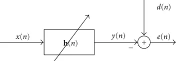
Figure 1 shows a typical adaptive filter setup, where x(n),

d(n), ande(n) are the input, the desired and the output error signals, respectively. Here,h(n) is theM×1 column vector of filter coeﬃcients at iterationn.

The generic filter vector update equation at the center of our analysis is introduced as

h(n+ 1)=h(n) +μC(n)X(n)W(n)e(n), (1)

where

e(n)=d(n)−XT₍_n₎_h₍_n₎ ₍₂₎

is the output error vector. The matrixX(n) is theM×Pinput signal matrix (The parameterPis a positive integer (usually, but not necessarilyP≤M)),

h(n) + −

y(n) _e(n)

x(n)

d(n)

Figure1: Prototypical adaptive filter setup.

X(n)=[x(n),x(n−1),. . .,x(n−(P−1))], (3)

wherex(n)=[x(n),x(n−1),. . .,x(n−M+ 1)]Tis the input signal vector, andd(n) is aP×1 vector of desired signal

d(_n)=[_d(_n),_d(_n−1),. . .,d(_n−(_P−1))]T. (4) The desired signal is assumed to be generated from the following linear model:

d(n)=XT₍_n₎_h

t(n) +v(n), (5)

where v(n) = [v(n),v(n−1),. . .,v(n−(P −1))]T is the measurement noise vector and assumed to be zero mean, white, Gaussian, and independent of the input signal, and ht(n) is the unknown filter vector which is time-variant. We assume that the variation ofh_t(n) is according to the random walk model [1,2,25]

ht(n+ 1)=ht(n) +q(n), (6) where the sequence ofq(n) is an independent and identically distributed sequence with autocorrelation matrix Q =

E{q(n)qT₍_n₎_}_{and independent of the}_x₍_k_{) for all}_k_{and of} thed(k) fork < n.

3. Derivation of SPU Adaptive Filter Algorithms

Diﬀerent adaptive filter algorithms are established through the specific choices for the matricesC(n) andW(n) as well as for the parameterP.

3.1. The Family of SPU-NLMS Algorithms. From (1), the generic filter coeﬃcients update equation forP = 1 can be stated as

h(n+ 1)=h(n) +μC(n)x(n)W(n)e(n). (7) In the adaptive filter algorithms with selective partial updates, theM×1 vector of filter coeﬃcients is partitioned into K blocks each of length L and in each iteration a subset of these blocks is updated. For this family of adaptive filters, the matrices C(n) and W(n) can be obtained from

Table 1, where theA(n) matrix is theM×Mdiagonal matrix

(3)

Table1: Family of adaptive filters with selective partial updates.

Algorithm P L K N C(n) W(n)

Max-NLMS [22] 1 1 M 1 A(n) 1

A(n)x(n)2

N-Max NLMS [16,23] 1 1 M N≤M A(n) 1

x(n)2

SPU-NLMS [24] 1 L M/L N≤K A(n) 1

x(n)2

SPU-NLMS [17,18] 1 1 M N≤M A(n) 1

A(n)x(n)2

SPU-NLMS [17] 1 L M/L 1 A(n) 1

A(n)x(n)2

SPU-NLMS [17] 1 L M/L N≤K A(n) 1

A(n)x(n)2

SPU-APA [17] P≤M L M/L N≤K A(n) (XT₍_n₎_A₍_n₎_X₍_n₎₎−1

the matricesC(n) andW(n), diﬀerent SPU-NLMS adaptive filter algorithms are established.

By partitioning the regressor vectorx(n) intoK blocks each of lengthLas

x(_n)=xT1(n),xT2(n),. . .,xKT(n) T

, (8)

the positions of 1 blocks (N blocks and N ≤ K) on the diagonal of A(n) matrix for each iteration in the family of SPU-NLMS adaptive algorithms are determined by the following procedure:

(1) thexi(n)2values are sorted for 1≤i≤K;

(2) theivalues that determine the positions of1blocks correspond to theNlargest values ofxi(n)2.

3.2. The SPU-APA. The filter vector update equation for SPU-APA is given by [17]

hF(n+ 1)=hF(n) +μXF(n)

XT_F(n)XF(n) −1

e(n), (9)

whereF= {j1,j2,. . .,jN}denote the indices of theNblocks out ofKblocks that should be updated at every adaptation, and

XF(n)=

XT_j₁(_n),XT_j₂(_n),_{. . .},XT_j_N(_n)T (10)

is theNL×Pmatrix and

Xi(n)=[xi(n),xi(n−1),. . .,xi(n−(P−1))] (11) is theL×P matrix. The indices ofF are obtained by the following procedure:

(1) compute the following values for 1≤i≤K

TrXT

i(n)Xi(n)

; (12)

(2) the indices ofFare correspond toNlargest values of (12).

From (9), the SPU-PRA can also be established when the adaptation of the filter coeﬃcients is performed only once everyP iterations. Equation (9) can be represented in the form of full update equation as

h(n+ 1)=h(n) +μA(n)X(n)XT₍_n₎_A₍_n₎_X₍_n₎−1_e₍_n_), (13)

where theA(n) matrix is theM×Mdiagonal matrix with the1and0blocks each of lengthLon the diagonal and the positions of 1’s on the diagonal determine which coeﬃcients should be updated in each iteration. The positions of1blocks (Nblocks andN ≤ K) on the diagonal ofA(n) matrix for each iteration in the SPU-APA is determined by the indices

of F.Table 1 summarizes the parameters selection for the

establishment of SPU-APA.

4. Tracking Performance Analysis of the Family

of SPU-NLMS and SPU-APA

The steady-state mean square error (MSE) performance of adaptive filter algorithms can be evaluated from (14):

MSE= lim n→ ∞E

e2₍_n₎_.

(14)

In this section, we apply the energy conservation arguments approach to find the steady-state MSE of the family of SPU-NLMS and SPU-AP adaptive filter algorithms. By defining the weight error vector as

h(_n)=ht(n)−h(n), (15) equation (1) can be stated as

ht(n+ 1)−h(n+ 1)=ht(n+ 1)−h(n)

−μC(n)X(n)W(n)e(n). (16)

Substituting (6) into (16) yields

ht(n+ 1)−h(n+ 1)=ht(n)−h(n) +q(n)

(4)

Therefore, (17) can be written as

h(n+ 1)=h(n) +q(n)−μC(n)X(n)W(n)e(n). (18)

By multiplying both sides of (18) from the left byXT₍_n_{), we} obtain

ep(n)=ea(n)−μXT(n)C(n)X(n)W(n)e(n), (19)

where ea(n) and ep(n) are a priori and posteriori error vectors which are defined as

ea(n)=XT(n)(ht(n+ 1)−h(n))

=XT₍_n₎ _h

t(n) +q(n)−h(n)

=XT(n)h(n) +q(n),

ep(n)=XT(n)(ht(n+ 1)−h(n+ 1))

=XT(n)h(n+ 1).

(20)

Finding e(n) from (19) and substitute it into (18), the following equality will be established:

h(n+ 1) + (C(n)X(n)W(n))XT₍_n₎_C₍_n₎_X₍_n₎_W₍_n₎−1_e a(n)

=h(n) +q(n) + (C(n)X(n)W(n))

×XT₍_n₎_C₍_n₎_X₍_n₎_W₍_n₎−1_e p(n).

(21)

Taking the Euclidean norm and then expectation from both sides of (21) and using the random walk model (6), we obtain after some calculations, that in the nonstationary environment the following energy equality holds:

Eh(n+ 1)2

+EeT_a(n)W(n)Z−1(n)ea(n)

=Eh(n)2

+Eq(n)2

+EeT

p(n)W(n)Z−1(n)ep(n)

,

(22)

where Z(n) = XT₍_n₎_C₍_n₎_X₍_n₎_W₍_n_{). Using the following} steady-state condition,E{h(n+ 1)2_{} =}_E_{_h₍_n₎2_}_{, yields}

EeT_a(n)W(n)Z−1(n)ea(n)

=Eq(n)2+EeT

p(n)W(n)Z−1(n)ep(n)

.

(23)

Focusing on the second term of the right-hand side (RHS) of (23) and using (19), we obtain

EeT_p(n)W(n)Z−1(n)ep(n)

=EeT

a(n)W(n)Z−1(n)ea(n)

−μEeT_a(n)W(n)e(n)

−μEeT(n)ZT(n)W(n)Z−1(n)ea(n)

+μ2_E_eT₍_n₎_ZT₍_n₎_W₍_n₎_Z−1₍_n₎_e₍_n₎_.

(24)

By substituting (24) into the second term of RHS of (23) and eliminating the equal terms from both sides, we have

−μEeT_a(n)W(n)e(n)

−μEeT₍_n₎_ZT₍_n₎_W₍_n₎_Z−1₍_n₎_e a(n)

+μ2EeT(_n)ZT(_n)W(_n)Z−1(_n)e(_n)

+Eq(n)2=0.

(25)

From (2) and (5), the relation between the output estimation error and a priori estimation error vectors is given by

e(n)=e_a(n) +v(n). (26) Using (26), we obtain

−μEeT_a(n)W(n)ea(n)

−μEeT

a(n)ZT(n)W(n)Z−1(n)ea(n)

+μ2_E_eT

a(n)ZT(n)W(n)ea(n)

+μ2_E_vT₍_n₎_ZT₍_n₎_W₍_n₎_v₍_n₎_{+ Tr(}_Q₎₌₀_. (27)

The steady-state excess MSE (EMSE) is defined as

EMSE= lim n→ ∞E

e2a(n)

, ₍₂₈₎

whereea(n) is the a priori error signal. To obtain the steady-state EMSE, we need the following assumption from [12]. At steady-state the input signal and therefore Z(n) and W(n) are statistically independent of ea(n) and moreover

E{e_a(n)eT

a(n)} = E{e2a(n)} ·S whereS ≈ IP×P for smallμ andS≈(1·1T_{) for large}_μ_where₁T₌_{[1, 0,}_{. . .}_{, 0]}

1×P. Based on this, we analyze four parts of (27),

Part I:

EeT

a(n)W(n)ea(n)

=Ee2 a(n)

Tr(SE{W(n)}). (29)

Part II:

EeT_a(n)ZT(n)W(n)Z−1(n)ea(n)

=Ee2 a(n)

TrSEZT₍_n₎_W₍_n₎_Z−1₍_n₎_.

(5)

Part III:

EeT_a(n)ZT(n)W(n)ea(n)

=Ee2 a(n)

TrSEZT₍_n₎_W₍_n₎_.

(31)

Part IV:

EvT(_n)ZT(_n)W(_n)v(_n)=σv2Tr

EZT(_n)W(_n)_. (32)

Therefore from (27), the EMSE is given by

Ee2 a(n)

=EMSE= μσv2Tr E

ZT₍_n₎_W₍_n₎₊_μ−1_Tr(_Q₎

Tr(SE{W(n)}) + Tr(SE{ZT₍_n₎_W₍_n₎_Z−1₍_n₎_}₎₋_μ_Tr(_S_E_{_ZT₍_n₎_W₍_n₎_}₎. (33)

Also from (26), the steady-state MSE can be obtained by

MSE=EMSE +σv2. (34) From the general expression (33), we will be able to predict the steady-state MSE of the family of NLMS, and SPU-AP adaptive filter algorithms in the nonstationary environ-ment. Selecting A(n) = I and the parameters selection according toTable 1, the tracking performance of NLMS and APA can also be analyzed.

5. Simulation Results

The theoretical results presented in this paper are confirmed by several computer simulations for a system identification setup. The unknown systems have 8 and 16, where the taps are randomly selected. The input signalx(n) is a first-order autoregressive (AR) signal generated by

x(n)=ρx(n−1) +w(n) (35) wherew(n) is either a zero mean white Gaussian signal or a zero mean uniformly distributed random sequence between

−1 and 1. For the Gaussian case, the value of ρ is set to 0.9, generating a highly colored Gaussian signal. For the uniform distribution case, the value ofρ is set to 0.5. The measurement noisev(n) withσ2

v=10−3is added to the noise free desired signald(n)=hT

t(n)x(n). The adaptive filter and the unknown channel are assumed to have the same number of taps. In all simulations, the simulated learning curves are obtained by ensemble averaging over 200 independent trials. Also, the steady-state MSE is obtained by averaging over 500 steady-state samples from 500 independent realizations for each value of μfor a given algorithm. Also, we assume an independent and identically distributed sequence for q(n) with autocorrelation matrixQ=σ2

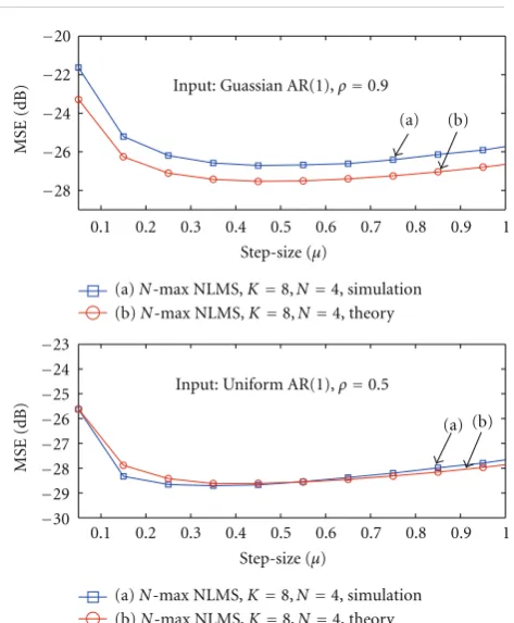
q·Iwhereσq2=0.0025σv2. Figures 2–5 show the steady-state MSE of the N-Max NLMS adaptive algorithm forM=8, and diﬀerent values for

Nas a function of step size in a nonstationary environment. The step size changes in the stability bound for both colored Gaussian and uniform distribution input signals. Figure 2 shows the results forN = 4, and for diﬀrent input signals. The theoretical results are from (33). As we can see, the theoretical values are in good agreement with simulation results. This agreement is better for uniform input signal.

Figure 3presents the results forN=5. Again, the agreement

is good, specially for uniform input signal. In Figures4and

0.1 0.2 0.3 0.4 0.5 0.6 0.7 0.8 0.9 1 −28

−26 −24 −22 −20

(a)N-max NLMS,K=8,N=4, simulation (b)N-max NLMS,K=8,N=4, theory

(a) (b) Input: Guassian AR(1),ρ=0.9

MSE

(dB)

Step-size (μ)

0.1 0.2 0.3 0.4 0.5 0.6 0.7 0.8 0.9 1

(a)N-max NLMS,K=8,N=4, simulation (b)N-max NLMS,K=8,N=4, theory −30

−29 −28 −27 −26 −25 −24 −23

(a) (b)

MSE

(dB)

Step-size (μ) Input: Uniform AR(1),ρ=0.5

Figure2: Steady-state MSE ofN-Max NLMS withM=8 andN=

4 as a function of the step size in nonstationary environment for diﬀerent input signals.

5, we presented the results forN=6, andN=7 respectively. This figure shows that the derived theoretical expression is suitable to predict the steady-state MSE of N-Max NLMS adaptive filter algorithm in nonstationary environment.

(6)

0.1 0.2 0.3 0.4 0.5 0.6 0.7 0.8 0.9 1 −28

−26 −24 −22 −20

MSE

(dB)

Step-size (μ)

0.1 0.2 0.3 0.4 0.5 0.6 0.7 0.8 0.9 1 −30

−29 −28 −27 −26 −25 −24 −23

MSE

(dB)

(a) (b)

0.1 0.2 0.3 0.4 0.5 0.6 0.7 0.8 0.9 1 −28

−26 −24 −22 −20

Input: Guassian AR(1),ρ=0.9

MSE

(dB)

(a) (b)

Step-size (μ)

0.1 0.2 0.3 0.4 0.5 0.6 0.7 0.8 0.9 1 −30

−29 −28 −27 −26 −25 −24 −23

(a) (b)

MSE

(dB)

0.1 0.2 0.3 0.4 0.5 0.6 0.7 0.8 0.9 1 −28

−26 −24 −22 −20

MSE

(dB) (a) _(b)

Step-size (μ)

−28 −26 −24 −22 −20

MSE

(dB)

−30

0.1 0.2 0.3 0.4 0.5 0.6 0.7 0.8 0.9 1 (a) (b)

0.1 0.2 0.3 0.4 0.5 0.6 0.7 0.8 0.9 1 −28

−26 −24 −22 −20

MSE

(dB) (a) (b)

(a) SPU-NLMS,M=8,K=4,N=2, simulation Step-size (μ)

(b) SPU-NLMS,M=8,K=4,N=2, theory

(a) (b)

−28 −26 −24 −22

MSE

(dB)

−30

0.1 0.2 0.3 0.4 0.5 0.6 0.7 0.8 0.9 1

(a) SPU-NLMS,M=8,K=4,N=2, simulation Step-size (μ)

Input: Uniform AR(1),ρ=0.5

(b) SPU-NLMS,M=8,K=4,N=2, theory

(7)

0.1 0.2 0.3 0.4 0.5 0.6 0.7 0.8 0.9 1 −28

−26 −24 −22 −20

MSE

(dB) (a) (b)

(a) SPU-NLMS,M=8,K=4,N=3, simulation (b) SPU-NLMS,M=8,K=4,N=3, theory

Step-size (μ)

0.1 0.2 0.3 0.4 0.5 0.6 0.7 0.8 0.9 1 −30

−29 −28 −27 −26 −25 −24 −23

MSE

(dB)

(a) (b)

Figure7: Steady-state MSE of SPU-NLMS withM=8,K=4 and N =3 as a function of the step size in nonstationary environment for diﬀerent input signals.

0.1 0.2 0.3 0.4 0.5 0.6 0.7 0.8 0.9 1 −28

−26 −24 −22 −20

MSE

(dB) (a) _(b)

Step-size (μ)

−28 −26 −24 −22 −20

MSE

(dB)

−30

0.1 0.2 0.3 0.4 0.5 0.6 0.7 0.8 0.9 1 (a)

(b)

Figure8: Steady-state MSE of SPU-NLMS withM=8,K=4 and N =4 as a function of the step size in nonstationary environment for diﬀerent input signals.

0 0.1 0.2 0.3 0.4 0.5 0.6 0.7 0.8 0.9 1 −28

−27 −26 −25 −24 −23 −22

(a) SPU-APA,M=8,P=4,K=4,N=2, simulation (b) SPU-APA,M=8,P=4,K=4,N=2, theory

MSE

(dB)

(a) (b)

Step-size (μ)

0 0.1 0.2 0.3 0.4 0.5 0.6 0.7 0.8 0.9 1 −30

−29 −28 −27 −26

MSE

(dB)

(a) (b)

Figure 9: Steady-state MSE of SPU-APA withM = 8,P = 4, K = 4 andN =2 as a function of the step size in nonstationary environment for diﬀerent input signals.

0 0.1 0.2 0.3 0.4 0.5 0.6 0.7 0.8 0.9 1 −29

−28 −27 −26 −25 −24

MSE

(dB)

Step-size (μ)

0 0.1 0.2 0.3 0.4 0.5 0.6 0.7 0.8 0.9 1 −29.5

−29 −28.5 −28 −27.5 −27 −26.5

MSE

(dB)

(a) (b)

(8)

MSE

(dB) (a)

(b)

−29 −28 −27 −26 −25

0 0.1 0.2 0.3 0.4 0.5 0.6 0.7 0.8 0.9 1 Input: Guassian AR(1),ρ=0.9

Step-size (μ)

0 0.1 0.2 0.3 0.4 0.5 0.6 0.7 0.8 0.9 1 −30

−29 −28 −27 −26

MSE

(dB)

(a) (b)

Figure11: Steady-state MSE of SPU-APA with M = 8,P = 4, K =4 andN =4 as a function of the step size in nonstationary environment for diﬀerent input signals.

0 500 1000 1500 2000 2500 3000 −30

−25 −20 −15 −10 −5 0 5 10 15

Iteration

10

log(MSE)

dB

(a)

(a)N-max NLMS,K=8,N=4,μ=0.2 (b)N-max NLMS,K=8,N=4,μ=0.4 (c)N-max NLMS,K=8,N=4,μ=0.6 Theoretical

(b) (c)

Figure12: Learning curves ofN-Max NLMS withM=8 andN=

4 and diﬀerent values of the step size for colored Gaussian input signal.

0 500 1000 1500 2000 2500 3000 −30

−25 −20 −15 −10 −5 0 5 10 15

Iteration

10

log(MSE)

dB

(a)

Theoretical (b) (c)

Input: Guassian AR(1),μ=0.9

(a) SPU-NLMS,M=8,K=4,N=4,μ=0.1 (b) SPU-NLMS,M=8,K=4,N=3,μ=0.1 (c) SPU-NLMS,M=8,K=4,N=2,μ=0.1

Figure13: Learning curves of SPU-NLMS withM=8,K=4, and N=2, 3, 4 for colored Gaussian input signal.

0 500 1000 1500 2000 2500 3000 −30

−25 −20 −15 −10 −5 0 5 10 15

Iteration

10

log(MSE)

dB

(a)

Theoretical

(b) (c)

(a) SPU-NLMS,M=8,K=4,N=3,μ=0.1,σ2

q=0.0025σv2

(b) SPU-NLMS,M=8,K=4,N=3,μ=0.1,σ2

q=0.025σv2

(c) SPU-NLMS,M=8,K=4,N=3,μ=0.1,σ2

q=0.0015σv2

(9)

−5

−25 −20 −15 −10

(a) SPU-NLMS,M=16,K=4,N=2, simulation (b) SPU-NLMS,M=16,K=4,N=2, theory 0 0.1 0.2 0.3 0.4 0.5 0.6 0.7 0.8 0.9 1

MSE

(dB) (a)

(b)

Step-size (μ)

−25 −20 −15 −10

−30

(a) SPU-NLMS,M=16,K=4,N=2, simulation (b) SPU-NLMS,M=16,K=4,N=2, theory 0 0.1 0.2 0.3 0.4 0.5 0.6 0.7 0.8 0.9 1

MSE

(dB) (a)_(b)

Figure15: Steady-state MSE of SPU-NLMS with M = 16,K =

4 and N = 2 as a function of the step size in nonstationary environment for diﬀerent input signals.

0 0.1 0.2 0.3 0.4 0.5 0.6 0.7 0.8 0.9 1

MSE

(dB) _(a)

(b)

−25 −20 −15 −10

Step-size (μ)

MSE

(dB) (a)

(b)

−28 −26 −24 −22 −20 −18 −16 −14

0 0.1 0.2 0.3 0.4 0.5 0.6 0.7 0.8 0.9 1

Figure16: Steady-state MSE of SPU-NLMS with M = 16,K =

4, and N = 3 as a function of the step size in nonstationary environment for diﬀerent input signals.

0 0.1 0.2 0.3 0.4 0.5 0.6 0.7 0.8 0.9 1

MSE

(dB)

(a) (b)

−24 −22 −20 −18 −16 −14 −12

Step-size (μ)

0 0.1 0.2 0.3 0.4 0.5 0.6 0.7 0.8 0.9 1

MSE

(dB) (a)

(b)

−28 −26 −24 −22 −20 −18 −16 −14

Figure17: Steady-state MSE of SPU-NLMS withM = 16,K =

4, and N = 4 as a function of the step size in nonstationary environment for diﬀerent input signals.

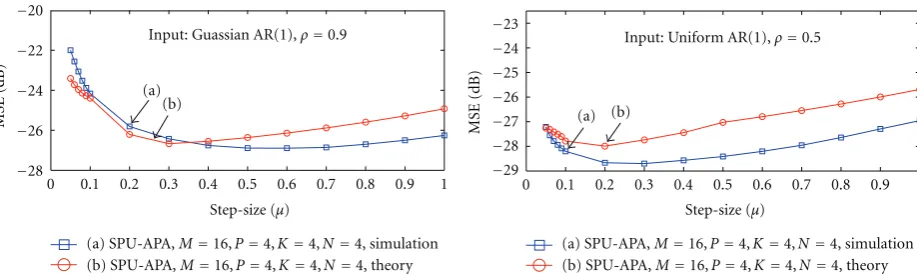
Figures9–11show the steady-state MSE of SPU-APA as a function of step size forM =8, and diﬀerent input signals. The parameters K, and P were set to 4, and the step size changes from 0.05 to 1. Diﬀerent values for N have been used in simulations.Figure 9shows the results forN = 2. Simulation results show good agreement for both colored and uniform input signals. InFigure 10, we set the parameter

N to 3. Again good agreement can be seen especially for uniform input signal. Finally,Figure 11shows the results for

N = 4. As we can see, the presented theoretical relation is suitable to predict the steady-state MSE.

Figures 12–14 show the simulated learning curves of SPU adaptive filter algorithms for diﬀerent parameters values and for colored Gaussian input signal. Figure 12 presents the learning curves forN-Max NLMS algorithm withM =

8, N = 4 and diﬀerent values for the step size. Also, the theoretical steady-state MSE was calculated based on (33) and compared with simulated steady-state MSE. As we can see the theoretical values are in good agreement with simulation results. Figure 13 shows the learning curves of SPU-NLMS algorithm withM=8,K =4, andN =2, 3, 4. Also, the step size was set to 0.1. Again the theoretical values of the steady-state MSE has been shown in this figure. Again good agreement is observed. InFigure 14, the learning curves of SPU-NLMS with M = 8, K = 4, and N = 3, have been presented for diﬀerent values of σ2

q. The degree of nonstationary changes by selecting diﬀerent values forσ2

q. As we can see, for the large values ofσ2

(10)

0 0.1 0.2 0.3 0.4 0.5 0.6 0.7 0.8 0.9 1

MSE

(dB)

−27 −26 −25 −24 −23 −22 −21

(a) (b)

Step-size (μ)

0 0.1 0.2 0.3 0.4 0.5 0.6 0.7 0.8 0.9 1

MSE

(dB)

−29 −28 −27 −26 −25 −24 −23

(a) (b)

Figure18: Steady-state MSE of SPU-APA withM=16,P=4,K=4, andN=3 as a function of the step size in nonstationary environment for diﬀerent input signals.

0 0.1 0.2 0.3 0.4 0.5 0.6 0.7 0.8 0.9 1

MSE

(dB)

−28 −26 −24 −22 −20

(a) (b)

Step-size (μ)

0 0.1 0.2 0.3 0.4 0.5 0.6 0.7 0.8 0.9 1

MSE

(dB)

−29 −28 −27 −26 −25 −24 −23

(a) (b)

Figure19: Steady-state MSE of SPU-APA withM=16,P=4,K=4, andN=4 as a function of the step size in nonstationary environment for diﬀerent input signals.

simulated steady-state MSE and theoretical steady-state MSE is deviated.

Figures15–17show the steady-state MSE of SPU-NLMS adaptive algorithm withM = 16 as a function of step size in a nonstationary environment for colored Gaussian and uniform input signals. We set the number of blocks (K) to 4 and diﬀerent values forN are chosen in simulations.

Figure 15 presents the results forN = 2 and for diﬀerent

input signals. The good agreement between the theoretical steady-state MSE and the simulated steady-state MSE is observed. In Figures16and17, we presented the results for

N =3, and 4. Simulation results show good agreement for both colored and uniform input signals.

Figures 18 and 19 show the steady-state MSE of SPU-APA as a function of step size for M = 16, and diﬀerent input signals. The parameters K, andP were set to 4, and the step size changes from 0.04 to 1. Diﬀerent values forN

have been used in simulations. Figure 18shows the results for N = 3. In Figure 19, the parameter N was set to 4. Again good agreement can be seen for both input signals.

The simulation results show that the agreement is deviated forM=16.

6. Summary and Conclusions

We presented a general framework for tracking performance analysis of the family of SPU-NLMS adaptive filter algo-rithms in nonstationary environment. Using the general expression and for the parameter values inTable 1, the mean square performances of Max-NLMS, N-Max NLMS, the various types of SPU-NLMS, and SPU-APA can be analyzed in a unified way. We demonstrated the usefulness of the presented analysis through several simulation results.

References

[1] B. Widrow and S. D. Stearns, Adaptive Signal Processing, Prentice Hall, Englewood Cliﬀs, NJ, USA, 1985.

(11)

[3] A. H. Sayed,Adaptive Filters, John Wiley & Sons, New York, NY, USA, 2008.

[4] B. Widrow, J. M. McCool, M. G. Larimore, and C. R. Johnson Jr., “Stationary and nonstationry learning characteristics of the LMS adaptive filter,”Proceedings of the IEEE, vol. 64, no. 8, pp. 1151–1162, 1976.

[5] N. J. Bershad, F. A. Reed, P. L. Feintuch, and B. Fisher, “Tracking charcteristics of the LMS adaptive line enhancer: response to a linear chrip signal in noise,”IEEE Transactions on Acoustics, Speech, and Signal Processing, vol. 28, no. 5, pp. 504–516, 1980.

[6] S. Marcos and O. Macchi, “Tracking capability of the least mean square algorithm: application to an asynchronous echo canceller,”IEEE Transactions on Acoustics, Speech, and Signal Processing, vol. 35, no. 11, pp. 1570–1578, 1987.

[7] E. Eweda, “Analysis and design of a signed regressor LMS algorithm for stationary and nonstationary adaptive filtering with correlated Gaussian data,”IEEE Transactions on Circuits and Systems, vol. 37, no. 11, pp. 1367–1374, 1990.

[8] E. Eweda, “Optimum step size of sign algorithm for non-stationary adaptive filtering,”IEEE Transactions on Acoustics, Speech, and Signal Processing, vol. 38, no. 11, pp. 1897–1901, 1990.

[9] E. Eweda, “Comparison of RLS, LMS, and sign algorithms for tracking randomly time-varying channels,”IEEE Transactions on Signal Processing, vol. 42, no. 11, pp. 2937–2944, 1994. [10] N. R. Yousef and A. H. Sayed, “Steady-state and tracking

analyses of the sign algorithm without the explicit use of the independence assumption,”IEEE Signal Processing Letters, vol. 7, no. 11, pp. 307–309, 2000.

[11] N. R. Yousef and A. H. Sayed, “A unified approach to the steady-state and tracking analyses of adaptive filters,” IEEE Transactions on Signal Processing, vol. 49, no. 2, pp. 314–324, 2001.

[12] H.-C. Shin and A. H. Sayed, “Mean-square performance of a family of aﬃne projection algorithms,”IEEE Transactions on Signal Processing, vol. 52, no. 1, pp. 90–102, 2004.

[13] A. H. Sayed and M. Rupp, “A time-domain feedback analysis of adaptive algorithms via the small gain theorem,” in Advanced Signal Processing Algorithms, vol. 2563 ofProceedings of SPIE, San Diego, Calif, USA, 1995.

[14] M. Rupp and A. H. Sayed, “A time-domain feedback analysis of filteredor adaptive gradient algorithms,”IEEE Transactions on Signal Processing, vol. 44, no. 6, pp. 1428–1439, 1996. [15] H.-C. Shin, W.-J. Song, and A. H. Sayed, “Mean-square

performance of data-reusing adaptive algorithms,”IEEE Signal Processing Letters, vol. 12, no. 12, pp. 851–854, 2005.

[16] T. Aboulnasr and K. Mayyas, “Complexity reduction of the NLMS algorithm via selective coeﬃcient update,” IEEE Transactions on Signal Processing, vol. 47, no. 5, pp. 1421–1424, 1999.

[17] K. Do˘ganc¸ay, “Adaptive filtering algorithms with selective partial updates,”IEEE Transactions on Circuits and Systems II: Analog and Digital Signal Processing, vol. 48, no. 8, pp. 762– 769, 2001.

[18] S. Werner, M. L. R. de Campos, and P. S. R. Diniz, “Partial-Update NLMS Algorithms with Data-Selective Updating,” IEEE Transactions on Signal Processing, vol. 52, no. 4, pp. 938– 949, 2004.

[19] M. S. E. Abadi and J. H. Husøy, “Mean-square performance of the family of adaptive filters with selective partial updates,” Signal Processing, vol. 88, no. 8, pp. 2008–2018, 2008.

[20] K. Do˘ganc¸ay,Partial-Update Adaptive Signal Processing, Design Analysis and implementation, Academic Press, New York, NY, USA, 2009.

[21] A. W.H. Khong and P. A. Naylor, “Selective-tap adaptive filtering with performance analysis for identification of time-varying systems,” IEEE Transactions on Audio, Speech and Language Processing, vol. 15, no. 5, pp. 1681–1695, 2007. [22] S. C. Douglas, “Analysis and implementation of the

max-NLMS adaptive filter,” inProceedings of the 29th Conference on Signals, Systems, and Computers, pp. 659–663, Pacific Grove, Calif, USA, October 1995.

[23] T. Aboulnasr and K. Mayyas, “Selective coeﬃcient update of gradient-based adaptive algorithms,” inProceedings of the 1997 IEEE International Conference on Acoustics, Speech, and Signal Processing (ICASSP ’97), pp. 1929–1932, Munich, Germany, April 1997.

[24] T. Schertler, “Selective block update of NLMS type algo-rithms,” inProceedings of the IEEE International Conference on Acoustics, Speech and Signal Processing (ICASSP ’98), pp. 1717– 1720, Seattle, Wash, USA, May 1998.