Volume 2008, Article ID 254573,17pages doi:10.1155/2008/254573
Research Article
Diversity Analysis of Distributed Space-Time Codes in Relay
Networks with Multiple Transmit/Receive Antennas
Yindi Jing1and Babak Hassibi2
1Department of Electrical Engineering and Computer Science, University of California, Irvine, CA 92697, USA 2Department of Electrical Engineering, California Institute of Technology, Pasadena, CA 91125, USA
Correspondence should be addressed to Yindi Jing,[email protected]
Received 1 May 2007; Revised 13 September 2007; Accepted 28 November 2007
Recommended by M. Chakraborty
The idea of space-time coding devised for multiple-antenna systems is applied to the problem of communication over a wireless relay network, a strategy calleddistributed space-time coding, to achieve the cooperative diversity provided by antennas of the relay nodes. In this paper, we extend the idea of distributed space-time coding to wireless relay networks with multiple-antenna nodes and fading channels. We show that for a wireless relay network withMantennas at the transmit node,Nantennas at the receive node, and a total ofRantennas at all the relay nodes, provided that the coherence interval is long enough, the high SNRpairwise error probability(PEP) behaves as (1/P)min{M,N}RifM /=N and (log1/MP/P)MRifM =N, wherePis the total power consumed by the network. Therefore, for the case ofM /=N, distributed space-time coding achieves the maximal diversity. For the case of M=N, the penalty is a factor of log1/MPwhich, compared toP, becomes negligible whenPis very high.
Copyright © 2008 Y. Jing and B. Hassibi. This is an open access article distributed under the Creative Commons Attribution License, which permits unrestricted use, distribution, and reproduction in any medium, provided the original work is properly cited.
1. INTRODUCTION
It is known that multiple antennas can greatly increase the capacity and reliability of a wireless communication link in a fading environment using space-time coding [1–4]. Recently, with the increasing interestin ad hoc networks, researchers have been looking for methods to exploit spatial diversity using the antennas of different users in the network [5–
24]. Many cooperative strategies are proposed, for example, amplify-and-forward (AF) [11,13,14,16,21,23], decode-and-forward (DF) [9,10,14,16,22], and coded cooperation [15]. In [7], the authors proposed the use of space-time codes based on Hurwitz-Radon matrices in wireless relay networks. This work follows the strategy of [5], where the idea of space-time coding devised for multiple-antennasystems is applied to the problem of communication over a wire-less relay network. (Though having the same name, the distributed space-time coding idea in [5] is different from that in [14]. Similar ideas for networks with one and two relays have appeared in [6,11].) In [5], the authors consider wireless relay networks in which every node has a single antenna and the channels are fading, and use a cooperative strategy called distributed space-time coding by applying a
linear dispersion space-time code [25] among the relays. It is proved that without any channel knowledge at the relays, a diversity ofR(1−log logP/logP) can be achieved, where R is the number of relays and P is the total power consumed in the whole network. This result is based on the assumption that the receiver has full knowledge of the fading channels. Therefore, when the total transmit powerPis high enough, the wireless relay network achieves the diversity of a multiple-antenna system with R transmit antennas and one receive antenna, asymptotically. That is, antennas of the relays work as antennas of the transmitter although they cannot fully cooperate and do not have full knowledge of the transmit signal. After the appearance of [5], code designs for distributed space-time coding have been proposed in [26–
31] and the differential use of distributed space-time coding has been introduced in [32–35]. The references [36,37] ana-lyze the diversity-multiplexing tradeoffof distributed space-time coding. Distributed space-space-time coding in asynchronous networks is discussed in [38–43]. Other related papers can be found in [44–46].
more importantly, based on the pairwise error probability (PEP) analysis, we prove lower bounds on the diversity of this scheme. We use the same two-step transmission method in [5], where in one step the transmitter sends signals to the relays and in the other the relays encode their received signals into a linear dispersion space-time code and transmit to the receiver. For a wireless relay network withMantennas at the transmitter, N antennas at the receiver, and a total ofR antennas at all the relay nodes, our work shows that when the coherence interval is long enough, a diversity of min{M,N}RifM /=NandMR(1−(1/M)(log logP/logP)) ifM=Ncan be achieved, wherePis the total power used in the network. With this two-step protocol, it is easy to see that the errorprobability is determined by the worse of the two steps: the transmission from the transmitter to the relays and the transmission from the relays to the receiver. Therefore, whenM /=N, distributed space-time coding is optimal since the diversity of the first stage cannot be larger than MR, the diversity of a multiple-antenna system withMtransmit antennas andR receive antennas, and the diversity of the second stage cannot be larger than NR. When M = N, the penalty on the diversity, because the relays cannot fully cooperate and do not have full knowledge of the signal, is R(log logP/logP). When P is very high, it is negligible. Therefore, with distributed space-time coding, wireless relay networks achieve the same diversity of multiple-antenna systems, asymptotically.
The paper is organized as follows. In the following section, the network model and the generalized distributed space-time coding are explained in detail. A training scheme is also proposed. The PEP is first analyzed in Section 3. InSection 4, the diversity for the network with an infinite number of relays is discussed. Then, the diversity for the general case is obtained in Section 5. Section 6 contains the conclusion. Proofs of some of the technical theorems are given in Appendices A–D. In Appendix E, we discuss heterogeneous networks.
2. WIRELESS RELAY NETWORK
2.1. Network model and distributed space-time coding
We first introduce some notation. For a complex matrixA, A,At, andA∗denote the conjugate, the transpose, and the Hermitian ofA, respectively. detA, rankA, and trAindicate the determinant, rank, and trace ofA, respectively.Adenotes the vectorization ofAformed by stacking the columns ofX into a single column vector.In denotes the n×n identity matrix and 0m,n is them×n matrix with all zero entries. We often omit the subscripts when there is no confusion. log indicates the natural logarithm. · indicates the Frobenius norm. P and E indicate the probability and the expected value. g(x) = O(f(x)) means that limx→∞(g(x)/ f(x)) is a constant.h(x)= o(f(x)) means that limx→∞(h(x)/ f(x)) = 0.ais the minimal integer that is not less thana.
Consider a wireless network with R+ 2 nodes which are placed randomly and independently according to some distribution. As shown in Figure 1, there are one transmit node and one receive node. All the other R nodes work
Transmitter Receiver
Relays
f11
f1R
fM1
fMR
g11
g1N . . . .
. . . . .
. . . .
. .
r1t1
rRtR
gR1
gRN
Step 1: time 1 toT Step 2: timeT+ 1 to 2T Figure1: Wireless relay network with multiple-antenna nodes.
as relays. The transmitter has M transmit antennas, the receiver has N receive antennas, and the ith relay has Ri antennas. Since the transmit and received signals at different antennas of the same relay can be processed and designed independently, the network can be transformed to a network
with R = R
i=1Ri single-antenna relays by designing the transmit signal at every antenna of every relay according to the received signal at that antenna only. This is one possible scheme. In general, the signal sent by one antenna of a relay can be designed using received signals at all antennas of the relay. However, as will be seen later, this simpler scheme achieves the optimal diversity asymptotically although a general design may improve the coding gain of the network. Therefore, to highlight the diversity results by simplifying notation and formulas, in the following, we assume that every relay has a single antenna. Denote the channel vector from theM antennas of the transmitter to the ith relay as fi = [f1i · · · fMi]t, and the channels from the ith relay to the N antennas at the receiver as gi = [gi1 · · · giN]. We use the block-fading model [2] by assuming a coherence intervalT. From the two-step protocol that will be discussed in the following, we can see that we only need fi to keep constant for the first step of the transmission andgito keep constant for the second step. It is thus good enough to choose T as the minimum of the coherence intervals offi andgi. Also, perfect symbol-level synchronization is assumed in this network model. For asynchronized networks, please refer to [38–43].
The information bits are encoded intoT×Mmatrices s, whosemth column is the signal sent by themth transmit antenna. For the power analysis,sis normalized as
E trs∗s=M. (1)
To sendsto the receiver, the same two-step strategy in [5] is used, as shown inFigure 1. In step one, the transmitter sends
P1T/Ms. The average total power used at the transmitter for theTtransmissions isP1T. The received signal vector and the noise vector at theith relay are denoted asriandvi. In step two, theith relay sendsti. The received signal and noise at the receiver are denoted asXandw. The noises are assumed to be i.i.d.CN(0, 1). Clearly,
ri=
P1T/Msfi+vi,
X=t1 · · · tR
G+w, (2)
whereG=[gt
We use distributed space-time coding proposed in [5] by designing the transmit signal at relayias a linear function of its received signal:
ti=
P2
P1+ 1Ai
ri, (3)
whereAiis a predeterminedT×Tunitary matrix known to both theith relay and the receiver. It is fixed during training and data transmissions. For various methods on how to design theAi, see [26–31].P2can be proved to be the average transmit power for one transmission at every relay. After some calculation, the system equation can be written as
X=
P1P2T
MP1+ 1
SH+W, (4)
where
S=A1s · · · ARs
, H=f1g1
t
· · · fRgR
tt ,
(5)
W =
P2
P1+ 1
⎡ ⎣R
i=1
gi1Aivi · · · R
i=1
giNAivi
⎤
⎦+w. (6)
The received signal matrix,X, isT×N.S, which isT×MR, is the linear distributed space-time code. SincefiisM×1 and giis 1×N, the equivalent channel matrixHisRM×N.W, which isT×N, is the equivalent noise matrix.
Define
RW =I+ P2 1 +P1G
∗G. (7)
The covariance matrix of the equivalent noise matrix can be proved to beRW. The diversity analysis in this paper is much more difficult than that in [5] because in networks with single-antenna nodes, the covariance matrix of the equivalent noise is a multiple of the identity matrix. Here, for the diversity result, we need to analyze the eigenvalues of RWor find bounds on them.
2.2. Assumptions and training
In this paper, we assume that fmiandgin have independent Rayleigh distributions; that is, fmi andgin are independent circulant complex Gaussian random variables with zero mean. For simplicity, we also assume that fmi andgin have the same variance, which is 1. The heterogeneous case, in which every channel has a different variance, is discussed in
Appendix E. The same diversity results can be obtained in heterogeneous networks. We make the practical assumption that the relays have no channel information. However, we do assume that the receiver has enough channel information to do coherent detection. Thus, a training process is needed.
For coherence ML decoding at the receiver, the receiver needs to know H andRW, or equivalently, H and G. We propose a training process that contains two steps and takes Mp+ 2Npsymbol periods (other training methods can also be envisioned, and the one proposed here is one possibility).
Each step mimics the training process of a multiple-antenna system [47] as its system equation has the same structure.
First, we estimateG, which takesMpsymbol periods. Let
Upbe a predesigned full-rankMp×Rpilot matrix. Theith relay sends theith column ofUpsimultaneously. The receiver gets
Yp=
QpMp
R UpG+wp, (8)
where Qp is the power used at every relay and wp is the Mp ×N noise matrix. Since there are RN unknowns (corresponding to the components ofG) and min{Mp,R}N independent equations, we needMp≥R. We could estimate
GfromUpusing ML, MMSE, or other criteria.
Then, we estimateHusing distributed space-time coding discussed inSection 2.1. This takes 2Npsymbol periods. The transmitter sends a full-rankNp×M pilot signal matrixsp and the relays perform distributed space-time coding. From (4), the received signal can be written as
Xp=
P1,pP2,pNp
M(P1,p+ 1)SpH
+Wp, (9)
whereP1,p andP2,p are the powers used at the transmitter and every relay and
Sp=
A1sp · · · ARsp
(10)
is the carefully designedNp×MRpilot space-time codeword. Now, let us discuss the number of training symbols needed in this step. Note thatGis known from the first training step. Define
f=f1t · · · fRt
t
. (11)
By stacking the columns ofXinto one single column vector, we can rewrite (9) as
Xp=
P1,pP2,pNp
MP1,p+ 1
⎡ ⎢ ⎢ ⎢ ⎢ ⎣
Spdiag
g11IM,. . .,gR1IM
.. .
Spdiag
g1NIM,. . .,gRNIM
⎤ ⎥ ⎥ ⎥ ⎥ ⎦f+Wp
=
P1,pP2,pNp
MP1,p+ 1
⎡ ⎢ ⎢ ⎢ ⎢ ⎣
g11A1sp · · · gR1ARsp ..
. . .. ...
g1NA1sp · · · gRNARsp
⎤ ⎥ ⎥ ⎥ ⎥ ⎦f+Wp
=
P1,pP2,pNp
MP1,p+ 1
⎡ ⎢ ⎢ ⎢ ⎢ ⎣
g11INp · · · gR1INp
..
. . .. ...
g1NINp · · · gRNINp
⎤ ⎥ ⎥ ⎥ ⎥ ⎦
×diagA1sp,. . .,ARsp
f+Wp.
Denote
Hp=
⎡ ⎢ ⎢ ⎣
g11INp · · · gR1INp
..
. . .. ... g1NINp · · · gRNINp
⎤ ⎥ ⎥
⎦diagA1sp,. . .,ARsp
.
(13)
The number of independent equations in (9) equals the rank of Hp, which is min{NpN,NpR,MR}. Since there areMR unknowns (corresponding to the components off), we need min{NpN,NpR,MR} ≥MR, which is equivalent to
Np≥max
MR/N,M. (14)
While this condition is satisfied, we could estimatef from Xpusing ML, MMSE, or other criteria. The overall training process takes at leastR+2 max{MR/N,M}symbol periods. The optimal designs ofUp,Qp,Sp(orsp), andP1,p,P2,pare interesting issues. However, they are beyond the scope of this paper.
3. PAIRWISE ERROR PROBABILITY AND OPTIMAL POWER ALLOCATION
To analyze the PEP, we have to determine the maximum-likelihood (ML)decoding rule. This requires the conditional
probability density function (PDF)P(X | sk), wheresk ∈S
andSis the set of all possible transmit signal matrices.
Theorem 1. Given thatskis transmitted, define
Sk=
A1sk A2sk · · · ARsk
. (15)
Then conditioned on sk, the rows of X are independently
Gaussian distributed with the same varianceRW. Thetth row
ofXhas meanP1P2T/M(P1+ 1)[Sk]tHwith[Sk]tbeing the
tth row ofSk. Also,
PX|sk
=πNdetRW
−T
×e−tr(X−
P1P2T/M
P1+1
SkH)R−W1(X−
P1P2T/M
P1+1
SkH)∗
. (16)
Proof. SeeAppendix A.
In view ofTheorem 1, we should emphasize that for a wireless relay network with multiple antennas at the receiver, the columns ofXare not independent although the rows of Xare. (The covariance matrix of each rowRWis not diagonal in general.) That is, the received signals at differentantennas
are not independent, whereas the received signals at different
timesare. This is the main reason that the PEP analysis in the new model is much more difficult than that of the network in [5], whereXhad only a single column.
With P(X|sk) in hand, we can obtain the ML decoding and thereby analyze the PEP. The result follows.
Theorem 2(ML decoding and the PEP Chernoff bound).
The ML decoding of the relay network is
arg min sk
tr
X−
P1P2T
MP1+ 1
SkH
×R−W1
X−
P1P2T
MP1+ 1
SkH
∗ .
(17)
With this decoding, the PEP of mistakingskbysl, averaged over
the channel realization, has the following upper bound:
Psk−→sl≤ E
fmi,gin
e−(P1P2T/4M(1+P1)) tr (Sk−Sl)∗(Sk−Sl)HR−W1H∗.
(18)
Proof. The proof is omitted since it is the same as the proof of Theorem 1 in [5].
As both H and RW are known at the receiver, sphere decoding can be used to perform the ML decoding in (17).
The main purpose of this work is to analyze how the PEP decays with the total transmit power. The total power used in the whole network isP=P1+RP2. One natural question is how to allocate power between the transmitter and the relays ifPis fixed. Notice that whenR→ ∞, according to the law of large numbers, the off-diagonal entries of (1/R)G∗Ggo to zero while the diagonal entries approach 1 with probability 1. It is thus reasonable to assume (1/R)G∗G ≈ IN for large
R. With this approximation, minimizing the PEP is now equivalent to maximizingP1P2T/4M(1 +P1+RP2). This is exactly the same power allocation problem in [5]. Therefore, we can conclude that the optimum solution is to set
P1=P
2, P2= P
2R. (19)
That is, the optimum power allocation is such that the transmitter uses half the total power and the relays share the other half. As discussed inSection 2.1, for the general network where the ith relay hasRi antennas, the antennas are treated as Ri different relays. Therefore, in general, the optimum power allocation is such that the transmitter uses half the total power as before, but every relay uses a power that is proportional to its number of antennas, that is,P1 =
P/2 and the power used at theith relay isRiP/2R.
4. DIVERSITY ANALYSIS FORR→ ∞
4.1. Basic results
have definedGn = diag{g1nIM,. . .,gRnIM}. Therefore, from (18) and using the optimal power allocation in (19),
Psk−→sl
E
fmi,gin
e−(PT/16MR)trH∗(Sk−Sl)∗(Sk−Sl)H
= E fmi,gin
e−(PT/16MR)Nn=1h∗n
Sk−Sl
∗
(Sk−Sl)hn
= E fmi,gin
e−(PT/16MR)f∗[N n=1G∗n
Sk−Sl
∗
(Sk−Sl)Gn]f.
(20)
Sincefis white Gaussian with mean zero and varianceIRM,
P(sk−→sl)
E gindet
−1
⎡
⎣IRM+ PT
16MR
N
n=1
G∗
n(Sk−Sl)∗(Sk−Sl)Gn
⎤ ⎦.
(21)
Similar to the multiple-antenna case [4, 48] and the case of wireless relay networks with single-antenna nodes [5], to achieve full diversity, Sk −Sl must be full rank. Since the distributed space-time codesSk andSl areT×MR, in the following, we will assume T ≥ MRand the code is fully diverse.
Denote the minimum singular value of (Sk−Sl)∗(Sk−
Sl) by σmin2 . From the full diversity of the code, σmin2 > 0. Therefore, the right side of (21) can be further upper bounded as
Psk−→sl
E
gin
det−1
⎡
⎣IRM+PTσmin2 16MR
N
n=1
G∗ nGn
⎤ ⎦
=E gin
R
i=1
⎛
⎝1 +PTσmin2 16MR
N
n=1
gin2
⎞ ⎠
−M
.
(22)
Since gin are i.i.d. CN(0, 1),
N
n=1|gin|2 are i.i.d. gamma distributed with PDF (1/(N−1)!)giN−1e−gi. Therefore,
Psk−→sl
1
(N−1)!R
⎡ ⎣∞
0
1 +PTσ 2 min 16MRx
−M
xN−1e−xdx
⎤ ⎦
R
.
(23)
By definingy=1 + (PTσ2
min/16MR)x, we have
Psk−→sl
1
(N−1)!R
16MR PTσ2
min
NR
e16MR2/PTσ2 min
×
∞
1
(y−1)N−1 yM e
−(16MR/PTσ2
min)yd y
R
1
(N−1)!R
16MR PTσ2
min
NR
×
⎡ ⎣N−1
l=0
N−1 l
∞
1 y
l−Me−(16MR/PTσ2
min)yd y
⎤ ⎦
R
.
(24)
The following theorem can be obtained by calculating the integral.
Theorem 3(diversity for R → ∞). Assume thatR → ∞, T ≥ MR, and the distributed space-time code is full diverse. For large total transmit powerP, by looking at only the highest-order term ofP, the PEP of mistakingskbyslhas the following
upper bound:
Psk−→sl 1
(N−1)!R
16MR Tσ2
min
min{M,N}R
×
⎧ ⎪ ⎪ ⎪ ⎪ ⎪ ⎪ ⎪ ⎪ ⎪ ⎪ ⎨ ⎪ ⎪ ⎪ ⎪ ⎪ ⎪ ⎪ ⎪ ⎪ ⎪ ⎩
2N−1
M−N
R
P−NR ifM > N,
log1/MP P
MR
ifM=N,
(N−M−1)!RP−MR ifM < N. (25)
Therefore, the diversity of the wireless relay network is
d=
⎧ ⎪ ⎪ ⎪ ⎪ ⎨ ⎪ ⎪ ⎪ ⎪ ⎩
min{M,N}R ifM /=N,
MR
1− 1 M
log logP logP
ifM=N.
(26)
Proof. SeeAppendix B.
4.2. Discussion
With the two-step protocol, it is easy to see that regardless of the cooperative strategy used at the relay nodes, the error probability is determined by the worse of the two transmission stages: the transmission from the transmitter to the relays and the transmission from the relays to the receiver. The PEP of the first stage cannot be better than the PEP of a multiple-antenna system withMtransmit antennas andR receive antennas, whose optimal diversity is MR, while the PEP of the second stage can have diversity not larger than NR. Therefore, when M /=N, according to the decay rate of the PEP, distributed space-time coding is optimal. For the case of M = N, the penalty on the decay rate is just R(log logP/logP), which is negligible whenPis high.
If we can use the diversity definition in [49], since limP→∞(log logP/logP) = 0, diversity min{M,N}Rcan be obtained.
therth term. When analyzing the diversity, not only is the first term important, but also how dominant it is. Therefore, we should analyze the contributions of the second and also other terms ofP compared to those of the first one. This is equivalent to analyzing how large the total transmit powerP should be for the terms in (25) to dominate. The following remarks are on this issue. They can be observed from the proof ofTheorem 3inAppendix B.
Remark 1. (1) If |M−N| > 1, from (B.13) and (B.22), the second term behaves as P−min{M,N}R+1. The difference between the first and second terms is aP factor. Therefore, the first term is dominant when P 1. In other words, contributions of the second and other terms are negligible whenP1.
(2) IfM=N, from (B.16), the second term is
2M−1R (M−1)!R
16MR Tσ2
min
MR logR−1P
PMR , (27)
which has one less logP than the first one. Therefore, the first term, (1/(M−1)!R)(16MR/Tσ2
min) MR
(log1/MP/P)MR, is dominant if and only if logP 1, which is a much stronger condition thanP 1. WhenP is not very large, contributions of the second and even other terms are not negligible.
(3) If |M − N| = 1, from (B.11) and (B.24), the second term behaves asP−min{M,N}R(logP/P). The difference between the first and second terms is logP/Pfactor. There-fore, the first term given in (25) is dominant if and only if P logP. This condition is weaker than the condition logP 1 in the previous case; however, it is still stronger than the normally used conditionP1.
5. DIVERSITY ANALYSIS FOR THE GENERAL CASE
5.1. A simple derivation
The diversity analysis in the previous section is based on the assumption that the number of relays is very large. In this section, analysis on the PEP and diversity for networks with any number of relays is given.
As discussed inSection 3, the main difficulty of the PEP analysis lies in the fact that the noise covariance matrixRW is not diagonal. From (18), we can see that one way of upper bounding the PEP is to upper boundRW. SinceRW≥0,
RW≤
trRW
IN=
⎛
⎝N+ P2
P1+ 1 N
n=1 R
i=1
gin2
⎞
⎠IN. (28)
Therefore, from (18) and using the power allocation given in (19),
Psk−→sl
E fmi,gin
e−(PT/8MNR(1+(1/NR)Nn=1 R
i=1gin
2
))trH∗(Sk−Sl)∗(S
k−Sl)H
(29)
whenP 1. If the space-time code is fully diverse, using similar argument in the previous section,
Psk−→slE gin
R
i=1
1 +PTσ 2 min 8MNR
gi 1 + (1/NR)Ri=1gi
−M ,
(30)
where, as before, σ2
min is the minimum singular value of (Sk−Sl)∗(Sk −Sl) and gi =
N
n=1|gin|2. Calculating this integral, the following theorem can be obtained.
Theorem 4 (diversity for wireless relay network). Assume thatT≥MRand the distributed space-time code is full diverse. For large total transmit powerP, by looking at the highest-order terms ofP, the PEP of mistakingskbyslsatisfies
P(sk−→sl) 1 (N−1)!R
8MNR Tσ2
min
min{M,N}R
×
⎧ ⎪ ⎪ ⎪ ⎪ ⎪ ⎪ ⎪ ⎪ ⎪ ⎪ ⎪ ⎪ ⎨ ⎪ ⎪ ⎪ ⎪ ⎪ ⎪ ⎪ ⎪ ⎪ ⎪ ⎪ ⎪ ⎩
M N(M−N)
R
P−NR ifM > N,
%
1 + 1 N
&Rlog1/MP
P
MR
ifM=N,
'
1
N + (N−M−1)!
(R
P−MR ifM < N. (31)
Therefore, the same diversity as in(26)is obtained. Proof. SeeAppendix C.
Although the same diversity is obtained as in theR → ∞ case, there is a factor of N in (31), which does not appear in (25). This is because we upper bound RW by (trRW)IN, whose expectation is N times the expectation of RW, while in the previous subsection we approximate
RW by its expectation. This factor ofN can be avoided by tighter upper bounds ofRW. In the following subsection, we analyze the maximum eigenvalue ofRW. Then inSection 5.3, a PEP upper bound using the maximum eigenvalue ofRWis obtained.
5.2. The maximum eigenvalue of Wishart matrix
Denote the maximum eigenvalue of (1/R)G∗Gasλmax. Since
G is a random matrix,λmax is a random variable. We first analyze the PDF and the cumulative distribution function (CDF)ofλmax.
0 0.5 1 1.5 2 2.5 3
Pr
(
λmax
=
λ
)
0 1 2 3 4 5
λ
R=10 N=2
R=10 N=3
R=10 N=4
R=40 N=2
R=40 N=3
R=40 N=4 PDF ofλmaxof Wishart matrix
Figure2: PDF of the maximum eigenvalue of (1/R)G∗G.
Theorem 5. Assume thatR ≥N andGis anR×Nmatrix whose entries are i.i.d.CN(0, 1).
(1) The PDF of the maximum eigenvalue of(1/R)G∗Gis
pλmax(λ)=
RRNλR−Ne−Rλ
)N
n=1Γ(R−n+ 1)Γ(n)
detF, (32)
whereFis an(N−1)×(N−1)Hankel matrix whose
(i,j)th entry equals fi j=
*λ 0(λ−t)
2
tR−N+i+j−2e−Rtdt. (2) The CDF of the maximum eigenvalue of(1/R)G∗Gis
Pλmax≤λ
=)N RRN
n=1Γ(R−n+ 1)Γ(n)
detF, (33)
whereFis anN×NHankel matrix whose(i,j)th entry equals fi j =
*λ
0tR−N+i+j−2e−Rtdt.
Proof. SeeAppendix D.
A theoretical analysis of the PDF and CDF from (32) and (33) appears to be quite difficult. To understandλmax, we plot the two functions in Figures2and3for differentR andN.Figure 2shows that the PDF has a peak at a value a bit larger than 1. AsRincreases, the peak becomes sharper. An increase inNshifts the peak right. However, the effect is smaller for largerR. FromFigure 3, the CDF ofλmaxgrows rapidly aroundλ=1 and becomes very close to 1 soon after. The largerRis, the faster the CDF grows. Similar to the PDF, an increase inNresults in a right shift of the CDF. However, asRgrows, the effect diminishes. This verifies the validity of the approximationG∗G≈RINinSection 4for largeR.
In the following corollary, we give an upper bound on the PDF. This result is used to derive the diversity result for generalRin the next subsection.
0 0.2 0.4 0.6 0.8 1
Pr
(
λmax
<λ
)
0 1 2 3 4 5
λ
R=10 N=2
R=10 N=3
R=10 N=4
R=40 N=2
R=40 N=3
R=40 N=4 CDF ofλmaxof Wishart matrix
Figure3: CDF of the maximum eigenvalue of (1/R)G∗G.
Corollary 1. When R ≥ N, the PDF of the maximum eigenvalue of(1/R)G∗Gcan be upper bounded as
pλmax(λ)≤C1λ
RN−1e−Rλ, (34)
where
C1=
1
)N
n=1Γ(R−n+ 1)Γ(n)
×)N−1 2N−1RRN
n=1(R−N+ 2n−1)(R−N+ 2n)(R−N+ 2n+ 1) (35)
is a constant that depends only onRandN.
Proof. From the proof of Theorem 5,Fis a positive semidef-inite matrix. Therefore, detF≤)N−1
n=1 fnn. From (32),fnncan be upper bounded as
fnn≤
λ
0
(λ−t)2tR−N+2n−2dt
= 2
(R−N+ 2n−1)(R−N+ 2n)(R−N+ 2n+ 1) ×λR−N+2n+1,
(36)
then we have
detF
≤)N−1 2N−1
n=1(R−N+ 2n−1)(R−N+ 2n)(R−N+ 2n+ 1) ×λRN−R+N−1.
(37)
5.3. Bound on PEP from bound on eigenvalues
If the maximum eigenvalue of (1/R)G∗Gisλmax, the maxi-mum eigenvalue ofRWis 1+(P2R/(P1+1))λmax, and therefore
RW ≤(1 + (P2R/(P1+ 1))λmax)IN. From (20) and using the power allocation given in (19), we have
Psk−→sl|λmax=c
≤ E fmr,grn
e−(P1P2T/4M(1+P1+P2Rλmax))tr(Sk−Sl)∗(Sk−Sl)HH∗
E
fmr,grn
e−(PT/8(1+λmax)MR)tr(Sk−Sl)∗(Sk−Sl)HH∗.
(38)
The only difference of the above formula with formula (20) is that the coefficient in the constant in the denominator of the exponent is 8(1 +λmax) now instead of 16. This makes sense sincec→1 asR→ ∞. Therefore, using an argument similar to the proof ofTheorem 3, at high total transmit power, by looking at the highest-order terms ofP,
Psk−→sl|λmax=c
1
(N−1)!R
8(1+c)MR Tσmin2
min{M,N}R
×
⎧ ⎪ ⎪ ⎪ ⎪ ⎪ ⎪ ⎪ ⎪ ⎪ ⎨ ⎪ ⎪ ⎪ ⎪ ⎪ ⎪ ⎪ ⎪ ⎪ ⎩
2N−1
M−N
R
P−NR ifM > N,
log1/MP P
MR
ifM=N,
(N−M−1)!RP−MR ifM < N. (39)
The following theorem can thus be obtained.
Theorem 6 (diversity for wireless relay network). Assume thatT≥MRand the distributed space-time code is full diverse. For large total transmit powerP, by looking at the highest-order terms ofP, the PEP of mistakingskbyslcan be upper bounded as
Psk−→sl C+ (N−1)!R
8MR Tσ2
min
min{M,N}R
×
⎧ ⎪ ⎪ ⎪ ⎪ ⎪ ⎪ ⎪ ⎪ ⎪ ⎪ ⎨ ⎪ ⎪ ⎪ ⎪ ⎪ ⎪ ⎪ ⎪ ⎪ ⎪ ⎩
2N−1
M−N
R
P−NR ifM > N,
log1/MP P
MR
ifM=N,
(N−M−1)!RP−MR ifM < N, (40)
where
+
C= ⎧ ⎪ ⎪ ⎪ ⎪ ⎪ ⎪ ⎪ ⎪ ⎪ ⎨ ⎪ ⎪ ⎪ ⎪ ⎪ ⎪ ⎪ ⎪ ⎪ ⎩
C1
min{M,N}R
i=0
⎛
⎝min{M,N}R
i
⎞
⎠(RN+i−1)!
RRN+i ifR≥N,
C2
min{M,N}R
i=0
⎛
⎝min{M,N}R
i
⎞
⎠(RN+i−1)!
RiNRN ifR<N,
C2=
1
)R
r=1Γ(N−r+ 1)Γ(r)
×)R−1 2R−1NRN
r=1(N−R+ 2r−1)(N−R+ 2r)(N−R+ 2r+ 1)
.
(41)
Therefore, the same diversity as in(26)is obtained.
Proof. WhenR≥N,
Psk−→sl=
∞
0
Psk−→sl|λmax=c
pλmax(c)dc
≤
∞
0 C1c
RN−1e−RcPs
k−→sl|λmax=c
dc (42)
using (34) inCorollary 1. From (39),
Psi−→si
C1 (N−1)!R
8MR Tσ2
min
min{M,N}R
×
∞
0 c
RN−1e−Rc(1 +c)min{M,N}R
dc
×
⎧ ⎪ ⎪ ⎪ ⎪ ⎪ ⎪ ⎪ ⎪ ⎪ ⎪ ⎨ ⎪ ⎪ ⎪ ⎪ ⎪ ⎪ ⎪ ⎪ ⎪ ⎪ ⎩
2N−1
M−N
R
P−NR ifM > N,
%logP
PM
&R
ifM=N,
(N−M−1)!RP−MR ifM < N. (43)
Since
∞
0 c
RN−1e−Rc(1 +c)min{M,N}R
dc
=
min{M,N}R
i=0
min{M,N}R i
(RN+i−1)! RRN+i ,
(44)
(40) is obtained.
For the case of R < N, G∗ is an N ×R (N > R) matrix whose entries are i.i.d.CN(0, 1). Denote the maximal eigenvalue of (1/N)GG∗asλmax. Its PDF and CDF are given inTheorem 5withRandNbeing switched. Using the facts that the maximal eigenvalue of (1/R)G∗Gis (N/R)λmaxand
∞
0 c
RN−1e−Nc
%
1 +N Rc
&min{M,N}R
dc
=
min{M,N}R
i=0
min{M,N}R i
(RN+i−1)! RiNRN ,
(45)
6. SIMULATION RESULTS
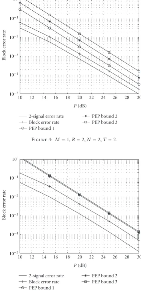
In this section, we show simulated block error rates of three networks with multiple transmit/receive antennas and compare them with the three PEP bounds we derived in (25), (31), and (40). These bounds are also addressed as PEP bound 1, PEP bound 2, and PEP bound 3 for the sake of presentation. The main purpose of this section is to verify the diversity results in (26). The optimal code design is not an issue. In the simulations, we use the power allocation in (19) and the ML decoding in (17). It is known that with ML metric, a factor of 1/2 can be applied to Chernoffbounds on the two-signal error rate, which is the block error rate when there are two possible transmit signals. Thus, the PEP bounds shown in Figures4–6are calculated from (25), (31), and (40) with a factor of 1/2. In all figures, the horizontal axis indicatesP, the total transmit power used in the whole network.
Our first example, whose performance is shown in
Figure 4, is a network with one transmit antenna, two relay antennas, and two receive antennas, that is,M =1,R= 2, N=2. We setT =MR=2. The transmit signal is designed as
s=s1 s2
t
, (46)
where s1 and s2 are chosen as BPSK signals (normalized according to (1)). The matrices used at relays are designed as
A1=I2, A2=
0 −1
1 0 . (47)
The distributed space-time codeword formed at the receiver Sis thus a 2×2 real orthogonal design [50]. Then, we show performance of a network withM = 2,R = 2,N = 1 in
Figure 5. We setT=MR=4. The transmit signal is deigned as
s=
⎡ ⎢ ⎢ ⎢ ⎣
s1 −s2
s2 s1
s3 −s4
s4 s3
⎤ ⎥ ⎥ ⎥
⎦, (48)
where s1, s2, s3, s4 are also BPSK signals (normalized according to (1)). The matrices used at relays are designed as
A1=I4, A2=
⎡ ⎢ ⎢ ⎢ ⎣
0 0 −1 0
0 0 0 1
1 0 0 0
0 1 0 0
⎤ ⎥ ⎥ ⎥
⎦. (49)
The distributed space-time codeword formed at the receiver S is thus a 4×4 real orthogonal design [50]. Finally, in
Figure 6, we show performance of a network withM = 2, R=1,N =2. We setT =MR =2. The transmit signal is
10−5 10−4 10−3 10−2 10−1 100
Blo
ck
er
ror
ra
te
10 12 14 16 18 20 22 24 26 28 30
P(dB) 2-signal error rate
Block error rate PEP bound 1
PEP bound 2 PEP bound 3
Figure4: M=1,R=2,N=2,T=2.
10−5 10−4 10−3 10−2 10−1 100
Blo
ck
er
ror
ra
te
10 12 14 16 18 20 22 24 26 28 30
P(dB) 2-signal error rate
Block error rate PEP bound 1
PEP bound 2 PEP bound 3
Figure5: M=2,R=2,N=1,T=4.
designed as
s=
s1 −s2
s2 s1 , (50)
10−5 10−4 10−3 10−2 10−1 100
Blo
ck
er
ror
ra
te
10 12 14 16 18 20 22 24 26 28 30
P(dB) 2-signal error rate
Block error rate PEP bound 1
PEP bound 2 PEP bound 3
Figure6: M=2,R=1,N=2,T=2.
Figures 4–6 indicate that when the transmit power is high, all three networks achieve the diversities shown by the PEP bounds. This verifies our diversity result in (26). PEP bound 1 is the tightest of the three. This is because PEP bound 1 is obtained by approximatingRW by its asymptotic (R→ ∞) limit, which is also its mean; however, strict lower bounds onRW are used in the calculations of bound 2 and bound 3. InFigure 5, the three bounds are very close to each other and, actually, bounds 1 and 2 are the same.
7. CONCLUSIONS
In this paper, we generalize the idea of distributed space-time coding to wireless relay networks whose transmitter, receiver, and/or relays can have multiple antennas. We assume that the channel information is only available at the receiver. The ML decoding at the receiver and PEP of the network are analyzed. We have shown that for a wireless relay network with M antennas at the transmitter,Nantennas at the receiver, a total ofRantennas at all the relay nodes, and a coherence interval not less thanMR, an achievable diversity is min{M,N}R
if M /=N andMR(1−(1/M)(log logP/logP)) ifM = N, where P is the total power used in the whole network. This result shows the optimality of distributed space-time coding according to the diversity gain. Simulation results are exhibited to justify our diversity analysis.
APPENDICES
A. PROOF OFTHEOREM 1
Proof. It is obvious that sinceHis known andWis Gaussian, the rows of X are Gaussian. We only need to show that the rows of X are uncorrelated and that the mean and variance of thetth row are(P1P2T/(P1+ 1)M)[Sk]tH and
RW, respectively.
The (t,n)th entry ofXcan be written as
xtn=
P1P2T
M(P1+ 1) R
i=1 M
m=1 T
τ=1
fmiginai,tτsk,τm
+
P2
P1+ 1 R
i=1 T
τ=1
ginai,tτviτ+wtn,
(A.1)
whereai,tτis the (t,τ)th entry ofAiandsk,τmis the (τ,m)th entry ofsk. With full channel information at the receiver,
Extn=
P1P2T
MP1+ 1
R
i=1 M
m=1 T
τ=1
fmiginai,tτsk,τm. (A.2)
Therefore, the mean of the tth row is then represented by
(P1P2T/M(P1+ 1))[Sk]tH. Sincevi,wn, and sk are inde-pendent,
Covxt1n1,xt2n2
=Ext1n1−Ext1n1
xt2n2−Ext2n2
= P2
P1+ 1 R
i1=1
T
τ1=1
R
i2=1
T
τ2=1
×Egi1n1ai1,t1τ1vr1τ1gi2n2ai2,t2τ2vi2τ2+ Ewt1n1wt2n2
= P2
P1+ 1 R
i=1 T
τ=1
ai,t1τai,t2τgin1gin2+δn1n2δt1t2
=δt1t2
⎛ ⎝ P2
P1+ 1 R
r=1
gin1gin2+δn1n2
⎞ ⎠
=δt1t2
⎛ ⎜ ⎜ ⎜ ⎜ ⎝
P2
P1+ 1
g1n1 · · · gRn1
⎛ ⎜ ⎜ ⎜ ⎜ ⎝
g1n2 .. .
gRn2
⎞ ⎟ ⎟ ⎟ ⎟ ⎠+δn1n2
⎞ ⎟ ⎟ ⎟ ⎟ ⎠.
(A.3)
The fourth equality is true sinceAiare unitary. Therefore, the rows ofXare independent since the covariance ofxt1n1 and xt2n2is zero whent1=/t2. It is also easy to see that the variance matrix of each row isIN+(P2/(P1+1))GtG, which equalsRW. Therefore,
P[X]t|sk
=.πNdetR W
/−T
×e−tr[X−√(P1P2T/M(P1+1))SkH]tR−W1[X−
√
(P1P2T/M(P1+1))SkH] t t
=.πNdetRW
/−T
×e−tr[X−√(P1P2T/M(P1+1))SkH]tR−W1[X−
√
(P1P2T/M(P1+1))SkH]
∗
t.
(A.4)
Since P(X | sk)=
)T
B. PROOF OFTHEOREM 3
Proof. Define
I= N−1
l=0
N−1 l
∞
1 y
l−Me−(16MR/PTσ2
min)yd y. (B.1)
We first give three integral equalities that will be used later:
∞
u x ne−μxdx
=e−uμ n
k=0
n! k!
uk
μn−k+1, u >0, Rμ >0, n=0, 1, 2,. . ., (B.2)
∞
u
e−μx
xn+1dx=(−1)
n+1μnEi(−μu)
n!
+e− μu
un n−1
k=0 (−1)k
μkuk
n· · ·(n−k), μ >0, n=1, 2,. . ., (B.3)
∞
u
e−μx
x dx= −Ei(−μu), Rμ >0, u≥0, (B.4) where
Ei(χ)=
χ
−∞ et
tdt, χ <0, (B.5) is the exponential integral function [51]. To calculate I, we discuss the following cases separately.
Case 1(M < N). In this case,
I= N−1
l=M
N−1 l
∞
1 y
l−Me−(16MR/PTσ2
min)yd y
+
⎛ ⎝N−1
M−1
⎞ ⎠∞
1
e−
16MR/PTσ2 min
y
y d y
+ M−2
l=0
⎛ ⎝N−1
l
⎞ ⎠∞
1 y
−(M−l)e−(16MR/PTσ2
min)yd y.
(B.6)
Using equalities (B.2)–(B.4) withu=1,μ=(16MR/PTσ2 min), andn=l−Morn=M−l−1,
I= N−1
l=M
N−1 l
(l−M)!
16MR PTσmin2
−(l−M+1)
+
N−1 M−1
logP+ M−2
l=0
N−1 l
1 M−l−1
+ lower-order terms ofP.
(B.7)
By only looking at the highest-order term ofP, which is in the first term withl=N−1, we have
I=(N−M−1)!
16MR PTσ2
min
−(N−M)
+o.P−(N−M)/. (B.8)
Therefore,
Psk−→sl
1
(N−1)!R
%
16MR PTσ2
min
&NR
×
'
(N−M−1)!
%
16MR PTσ2
min
&−(N−M) +o
%
1 PMR
&(R
=
'
(N−M−1)! (N−1)!
(R% 16MR Tσ2
min
&MR 1 PMR +o
%
1 PMR
&
. (B.9)
While analyzing the performance of the system at high transmit powerP, not only is the highest-order term ofP important, but also how fast other terms decay with respect to it. Therefore, we should also look at the second highest-order term ofP. To do this, we have to consider two different cases.
IfN=M+ 1,
I=
16MR PTσmin2
−1 +M
−Ei
−16MR PTσmin2
+O(1)
=
16MR PTσ2
min
−1
+MlogP+O(1).
(B.10)
Therefore,
Psk−→sl
1
M!R
16MR Tσ2
min
MR 1 PMR
+ RM M!R
16MR Tσ2
min
MR+1 logP PMR+1 +o
%
logP PMR+1
&
. (B.11)
The second highest-order term ofP in the PEP behaves as logP/PMR+1=P−(MR+1−log logP/logP).
IfN > M+ 1,
I=(N−M−1)!
%
16MR PTσ2
min
&−(N−M)
+ (N−1)(N−M−2)!
×
%
16MR PTσ2
min
&−(N−M−1)
+o.PN−M−1/
=
%
16MR PTσmin2
&−(N−M)'
(N−M−1)! + (N−1)
×(N−M−2)!16MR PTσmin2
+o
%
1 P
&(
Therefore,
Psk−→sl
(N−M−1)!R
(N−1)!R
%
16MR Tσmin2
&MR 1
PMR
+(N−1)(N−M−2)(N−M−1)! R−1
(N−1)!R
×
%
16MR Tσmin2
&MR+1 1
PMR+1 +o
%
1 PMR+1
&
. (B.13)
Case 2(M=N). In this case,
I=
∞
1
e−
16MR/PTσ2 min
y
y d y
+ N−2
l=0
N−1 l
∞
1 y
−(M−l)e−(16MR/PTσ2
min)yd y.
(B.14)
Using (B.4) withμ = 16MR/PTσ2
minandu = 1, and (B.3) withu=1 andn=M−l−1, we have
I=logP+ N−2
l=0
N−1 l
1 M−l−1
+ lower-order terms ofP
<logP+ 2N−1+ lower-order terms ofP.
(B.15)
Therefore,
Psk−→sl 1 (M−1)!R
%
16MR Tσ2
min
&MR logRP
PMR
+ 2
N−1R (M−1)!R
%
16MR Tσ2
min
&MRlogR−1P
PMR
+o
%
logR−1P PMR
&
.
(B.16)
Also, the second highest-order term ofPin the PEP behaves as logR−1P/PRM and the next term has one logPless and so on.
Case 3(M > N). In this case,
I= M−2
l=0
N−1 l
∞
1 y
−(M−l)e−(16MR/PTσ2
min)yd y. (B.17)
Using (B.3) withu=1,μ=16MR/PTσmin2 , andn=M−l−1,
I= N−1
l=0
N−1 l
1
M−l−1+ lower-order terms ofP. (B.18)
Thus,
Psk−→sl
1
(N−1)R
%
16MR PTσ2
min
&NR
×
N−1
l=0
N−1 l
1
M−l−1+o(1) R
=
1 (N−1)!
N−1
l=0
N−1 l
1 M−l−1
R
×
%
16MR Tσ2
min
&NR
P−NR+oP−NR.
(B.19)
We can further upper bound the PEP to get a simpler formula. Notice that 1/(M−l−1)≤1/(M−N). Thus,
Psk−→sl
1 (M−N)(N−1)!
N−1
l=0
N−1 l
R
×
%
16MR Tσmin2
&NR
P−NR
≤
'
2N−1 (M−N)(N−1)!
(R% 16MR Tσ2
min
&NR
P−NR. (B.20)
As discussed before, we also want to see how dominant the highest-order term ofPgiven in the above formula is. If M > N+ 1,M−l−2> N+ 1−(N−1)−2=0. From (B.3),
I < 2
N−1
M−N−
2N−1
(M−N)(M−N−1) 16MR PTσ2
min +o
%
1 P
&
. (B.21)
Therefore,
Psk−→sl
'
2N−1 (M−N)(N−1)!
(R% 16MR Tσ2
min
&NR
×
'
1 PNR+
R M−N−1
%
16MR Tσ2
min
&
1 PNR+1
(
+o
%
1 PNR+1
&
.
(B.22)
The second highest-order term in the PEP behaves as 1/(PNR+1). IfM=N+ 1,
I<2N−1+16MR
Tσ2 min
logP P +O
%
1 P
&
. (B.23)
Therefore,
Psk−→sl
2R(N−1)
(N−1)!R
%
16MR Tσmin2
&NR 1
PNR
+2
(R−1)(N−1)R (N−1)!R
%
16MR Tσ2
min
&NR+1 logP PNR+1
+o
%
logP PNR+1
&
,
which indicates that the second highest-order term in the PEP behaves as logP/PNR+1=R−(NR+1−log logP/logP).
C. PROOF OFTHEOREM 4
Proof. Sincegihave PDFp(gi)=(1/(N−1)!)giN−1e−gi,
Psk−→sl
≤ R
r=0
1≤i1<···<ir≤R
Ti1,...,ir, (C.1)
where
Ti1,...,ir=
1 (N−1)!R
· · ·
thei1,...,irth integrals are fromxto∞,
others are from 0 tox
× R
i=1
1 +PTσ 2 min 8MNR
gi 1 + (1/NR)Ri=1gi
−M
×gN−1
i e−gidg1· · ·dgR
(C.2)
andxis any positive real number. Let us calculateT1,...,rfirst:
T1,...,r= 1 (N−1)!R
∞
x . . .
∞
x
0 12 3
r
x
0 . . .
x
0
0 12 3
R−r R
i=1
×
1 +PTσ 2 min 8MNR
gi 1 + (1/NR)Ri=1gi
−M
×gN−1
i e−gidg1· · ·dgR
< 1 (N−1)!R
∞
x · · ·
∞
x r
i=1
×
PTσmin2 8MNR
gi
1 + ((R−r)/NR)x+ (1/NR)ri=1gi
−M
×giN−1e−gidg1· · ·dgr
×
x
0· · ·
x
0 R
i=r+1
giN−1e−gidgr+1· · ·dgR
= 1
(N−1)!R
%
PTσmin2 8MNR
&−rM
γR−r(N,x)
×
∞
x · · ·
∞
x
⎛
⎝1 +R−r NR x+
1 NR
r
i=1
gi
⎞ ⎠
rM
× r
i=1
e−gi
gM−N+1 i
dg1· · ·dgr,
(C.3)
where γ(n,x) is the incomplete gamma function [51]. We should choosex so that the diversity is maximized. Define x = βPα, where βis a positive constant and αis any real
constant. The value ofβdoes not affect the diversity. Here, to have the PEP result consistent with formula (25) inSection 6, we setβ=(Tσmin2 /8MNR)
α
. Therefore, choosing the optimal (in the sense of maximizing the diversity)xis equivalent to choosing the optimalα. Ifα >0, ther =0 term in the PEP upper bound is
1 (N−1)!Rγ
R(N,Pα)=1 +o(1). (C.4)
Therefore, having α positive is not optimal according to diversity. Similarly, ifα=0,x=1. Ther=0 term in the PEP upper bound, (1/(N−1)!R
)γR(N, 1), is a constant. Therefore,
αshould be negative. Thus,
γ(N,x)= 1 Nx
N+oxN= 1
Nβ
NPαN+oPαN (C.5)
We are only interested in the highest-order term ofP. When P is large, ((R−r)/NR)x is negligible compared with 1. Therefore,
T1,...,r
1 (N−1)!RNR−r
%
Tσmin2 8MNR
&−rM+αN(R−r)
×P−rM+αN(R−r)Λ,
(C.6)
where we have defined
Λ=
∞
x · · ·
∞
x
⎛ ⎝1 + 1
NR
r
i=1
gi
⎞ ⎠
rM r
i=1
e−gi
giM−N+1
dg1· · ·dgr.
(C.7)
We consider the expansion of (A+ki=1λi) a
into monomial terms:
%
1 + 1 NR
r
i=1
gi
&a =
a
j=0
1≤l1<···<lj≤k
i1,...,ij≥1
im≤a
Ci1,. . .,ij
× 1
(NR)i1+···+ijg
i1
l1g
i2
l2· · ·g
ij
lj
,
(C.8)
where j denotes how manygi are present,l1,. . .,lj are the subscripts of thegithat appear,im ≥ 1 indicates thatglm is
taken to theimth power, and finally
Ci1,. . .,ij
=
k i1
k−i1
i2
· · ·
k−i1− · · · −ij−1
ij
(C.9)
counts how many times the termgi1
l1g
i2
l2· · ·g
ij
lj appears in the
expansion. Thus,
Λ=
r
j=0
1≤l1<···<lj≤r
i1,...,ij≥1
im≤r
×Ci1,. . .,ij
Λj;l1,. . .,lj;i1,. . .,ij