Trellis-Based Iterative Adaptive Blind Sequence
Estimation for Uncoded/Coded Systems
with Differential Precoding
Xiao-Ming Chen
Information and Coding Theory Lab, Faculty of Engineering, University of Kiel, 24143 Kiel, Germany Email:[email protected]
Peter A. Hoeher
Information and Coding Theory Lab, Faculty of Engineering, University of Kiel, 24143 Kiel, Germany Email:[email protected]
Received 1 October 2003; Revised 23 April 2004
We propose iterative, adaptive trellis-based blind sequence estimators, which can be interpreted as reduced-complexity receivers derived from the joint ML data/channel estimation problem. The number of states in the trellis is considered as a design param-eter, providing a trade-offbetween performance and complexity. For symmetrical signal constellations, differential encoding or generalizations thereof are necessary to combat the phase ambiguity. At the receiver, the structure of the super-trellis (representing differential encoding and intersymbol interference) is explicitly exploited rather than doing differential decoding just for resolving the problem of phase ambiguity. In uncoded systems, it is shown that the data sequence can only be determined up to an unknown shift index. This shift ambiguity can be resolved by taking an outer channel encoder into account. The average magnitude of the soft outputs from the corresponding channel decoder is exploited to identify the shift index. For frequency-hopping systems over fading channels, a double serially concatenated scheme is proposed, where the inner code is applied to combat the shift ambiguity and the outer code provides time diversity in conjunction with an interburst interleaver.
Keywords and phrases:joint data/channel estimation, blind sequence estimation, iterative processing, turbo equalization.
1. INTRODUCTION
In most digital communication systems, a training sequence is inserted in each data burst for the purpose of channel esti-mation or for the adjustment of the taps of linear or decision-feedback equalizers. For an efficient usage of bandwidth, however, blind equalization techniques attract considerable attentions [1,2]. Furthermore, blind detection schemes may be embedded in existing systems as an add-on in order to improve the system performance in difficult environments.
Blind linear and nonlinear equalization techniques have been investigated since the pioneering work of Sato [3]. Con-ventionally, blind linear equalizers exploit the higher-order statistical relationship between the data signal and the equal-izer output signal. On-line adaptive algorithms based on the zero-forcing principle have been proposed in [3,4,5], for example. For burst-wise transmission, an iterative batch im-plementation of these algorithms is also possible [6], that is, the equalizer coefficients obtained at the end of one itera-tion are employed as the initial values in the next iteraitera-tion. Based on the minimum mean-square error (MMSE)
crite-rion, algorithms for blind identification and blind equaliza-tion have been proposed in [7,8] for multipath fading chan-nels. Possible drawbacks of linear blind equalizers are, de-pending on the algorithm, a slow convergence rate, a possible convergence to local minima, and a lack of robustness against Doppler spread, noise, and interference.
(e.g., based on least mean square (LMS), recursive least squares (RLS) or the Kalman algorithm [16]) are imple-mented in parallel to a blind trellis-based equalizer. Possible equalizers may be based on the Viterbi algorithm (VA), on per-survivor processing (PSP) [17], or on the list Viterbi al-gorithm (LVA) [18]. For equalizers based on the VA, a single-channel estimator is recursively updated by the locally best survivor given a suitable tentative decision delay [19, Chapter 11]. With PSP, each survivor employs its own channel esti-mator and no decision delay is afforded. In the LVA, for each trellis state, more than one survivor is maintained. Diff er-ent from the case with known channel coefficients, the num-ber of states in the trellis should be considered as a design parameter, which provides a trade-off between complexity and performance. In order to exploit statistical properties of the multipath fading channel and to track the time varia-tion of the channel, model-fitting algorithms were used in [20,21], for example. In this context, channel coefficients are modeled as complex Gaussian-distributed random variables, where the covariance matrix of channel coefficients are as-sumed to be known at the receiver. All these techniques can be applied straightforwardly to any tree-based sequential de-coding algorithm, for example, by means of the breadth-first sequential decoding algorithm as shown in [22]. In contrast to blind linear equalizers, all these trellis-based or tree-based approaches explicitly exploit the finite-alphabet property of data sequences.
The focus of this paper is on trellis-based blind sequence estimation for short burst sizes and noisy environments, where the only available channel knowledge is an upper bound on the channel order. Significant improvements with respect to acquisition and bit error rate (BER) performance are particularly obtained by incorporating on-line adaptive channel estimation into the equalizer, by performing itera-tive processing in the blind sequence estimator, and by us-ing a priori information about data symbols, for example, provided by an outer soft-output channel decoder or by ex-ploiting the residual correlation in the data sequence af-ter the source encoder [23]. As opposed to the optimal re-ceiver in the sense of MLSE, the reduced-complexity trellis-based blind sequence estimators considered here do not per-form an exhaustive search over all possible data hypotheses. Therefore, they may converge to local minima as observed in [12,13,14]. In this paper, we propose different approaches to combat phase ambiguity, shift ambiguity, and other local minima of the cost function. If the channel order is overde-termined, the data sequence can be only estimated up to an unknown shift index for uncoded systems. On the other hand, for coded schemes, this shift ambiguity can be resolved by exploiting code constraints. As opposed to the common understanding that differential encoding is used just to re-solve the phase ambiguity of channel and data estimation, we explicitly use the structure of the super-trellis. Besides in-corporating a priori information, the proposed trellis-based blind equalizer is also able to deliver soft outputs to subse-quent processing stages. Consesubse-quently, a blind turbo proces-sor can be obtained, which is composed of an inner blind soft-input soft-output (SISO) equalizer and an outer SISO
channel decoder. For blind turbo equalization of frequency-hopping systems over fading channels, we propose a novel transmitter/receiver structure with double serial concatena-tions. The inner concatenation is necessary to combat the shift ambiguity, while the outer concatenation exploits time diversity of channel codes in conjunction with an interburst interleaver.
InSection 2, we present the system model under investi-gation. Reduced-complexity trellis-based blind equalization techniques are derived from the ML joint data/channel es-timation problem inSection 3, which also shows the inher-ent relationship between these techniques. The initialization issue and techniques to combat local minima are discussed in Section 4. A summary of the proposed adaptive blind sequence estimator and simulation results for an uncoded GSM-like system are also presented inSection 4. Taking the outer channel decoder into consideration, we propose a blind turbo equalizer in Section 5, where the effect of phase/shift ambiguity on the coded system and corresponding solutions are also investigated. After providing numerical results for coded systems, some conclusions are drawn inSection 6.
2. SYSTEM MODEL
Throughout this paper we use the complex baseband nota-tion. In the following, (·)T, (·)∗, (·)H, and (·)† stand for transpose, complex conjugate, complex conjugate and trans-pose, and Moore-Penrose pseudo left inverse, respectively.
2.1. Transmitter
Within this paper, the focus is on anM-ary DPSK system. The task of the differential encoder is to resolve the phase am-biguity. The output symbols of the differential encoder can be written as
x[k]=x[k−1]d[k], x[0]=+1, 1≤k≤K, (1)
where d[k] areM-ary PSK data symbols with unit symbol energy,x[0]=+1 serves as a reference symbol, andKis the burst length (excluding the reference symbol). A generaliza-tion to other symmetrical signal constellageneraliza-tions with precod-ing (e.g., CPM) is possible.
2.2. Channel model
The pulse shaping filter, the frequency-selective channel, the receiving filter, and the sampling can be represented by a tapped-delay-line baud-rate model. (We restrict ourselves to baud-rate sampling. An extension to fractionally spaced sam-pling is straightforward. The validity of the tapped-delay-line model has been discussed for an unknown channel in [24, 25].) The corresponding outputs of the equivalent discrete-time channel model can be written as
y[k]=
L
l=0
hl[k]x[k−l] +n[k]
=xT[k]h[k] +n[k], 0≤k≤K,
d[k] x[k]
z−1 z−1
z−1 x[k−1]
x[k−1]
h1[k] h2[k] h0[k]
ISI channel +
DPSK/ISI superchannel
z[k]
+1, +1
+1,−1
−1, +1
−1,−1
+1, +1
+1,−1
−1, +1
−1,−1 x[k−2],x[k−1] x[k]/z[k] x[k−1],x[k]
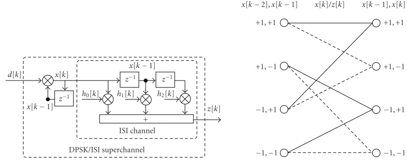
Figure1: ISI channel model and ISI trellis for the binary case withL=2.
whereh[k]=[hL[k],hL−1[k],. . .,h0[k]]Tis the time-varying channel coefficient vector with normalized power,Lis the ef-fective channel memory length after suitable truncation, and {n[k]} is assumed to be an additive white Gaussian noise (AWGN) sequence with varianceσ2
n per sample. Moreover, x[k]=[x[k−L],. . .,x[k]]T denotes the state transitions of thekth trellis segment.
For a burst-wise transmission, the channel model can be represented in vector/matrix notation as
y=Xh+n, (3)
where y = [y[0],. . .,y[K]]T,X = [x[0],. . .,x[K]]T, and n = [n[0],. . .,n[K]]T. Moreover,h = [h
L,. . .,h0]T is as-sumed to be constant within a burst. (If the data symbols are not transmitted on a burst-by-burst basis, if the burst size is large, or if the channel is fast time varying,Kmay denote the length of a subburst.)
2.3. Receiver
The task of the receiver based on the maximum-likelihood sequence estimation strategy is twofold. Primarily, we are interested in an estimate of the data vector d = [d[1],
d[2],. . .,d[K]]T. A pseudocoherent receiver (according to the definition in [26]) must also obtain estimates of each el-ement ofhin amplitude and phase.
In a pseudocoherent receiver, joint data/channel estima-tion may be based on the ISI trellis (followed by differential decoding), or may be based on the DPSK/ISI super-trellis, which combines the differential encoding and the ISI trel-lis. When differential encoding is used, a receiver based on the ISI trellis followed by differential encoding is equiva-lent to the receiver based on the super-trellis if and only if the transmitted symbols are independent and uniformly dis-tributed. If this is not the case, only the latter receiver can be optimal. In the following, only the latter receiver is investi-gated.
Figure 1 shows the ISI channel model and the corre-sponding ISI trellis for the case whenL = 2 and M = 2.
Taking the differential encoder into account, the equivalent DPSK/ISI superchannel and the corresponding DPSK/ISI super-trellis are depicted in Figure 2. Note that the num-ber of states is not increased by differential encoding. While the data symbol after differential encoding, namely,x[k], la-bels state transitions in the ISI trellis, the transition label changes to d[k] in the DPSK/ISI super-trellis. As indicated inFigure 2, the DPSK/ISI super channel can be interpreted as a recursive encoder, which is preferable for serially con-catenated turbo schemes [27]. In the following, our blind sequence estimator operates on the DPSK/ISI super-trellis. Furthermore, the differential encoder may be replaced by other recursive rate-1 precoders, which are able to combat the phase ambiguity, for example, any generalized diff eren-tial encoder shown in [28]. Although only the differential en-coder is considered within this paper, the proposed receiver can easily be extended to other suitable recursive precoders or modulation schemes with inherent differential encoding like CPM.
3. REDUCED-COMPLEXITY RECEIVERS DERIVED FROM THE ML JOINT DATA/CHANNEL ESTIMATOR
In this Section, reduced-complexity receivers for blind sequence estimation are derived from the ML joint data/channel estimation problem, where both data sequence and channel coefficients are unknown. Previously proposed algorithms are shown to be special cases of the proposed re-ceiver. In the following, ˜φandφdenote hypotheses and cor-responding estimates of φ, respectively, whereφ may be a scalar, a vector, or a matrix.
The ML joint data/channel estimation problem in the presence of AWGN can be formulated as
x,h=arg max ˜ x,˜h
py|x˜, ˜h=arg min ˜ X,˜h
y−X˜h˜2 , (4)
d[k] x[k]
z−1 z−1 h1[k] h2[k] h0[k]
ISI channel +
DPSK/ISI superchannel
z[k]
+1, +1
+1,−1
−1, +1
−1,−1
+1, +1
+1,−1
−1, +1
−1,−1 x[k−2],x[k−1] d[k]/z[k] x[k−1],x[k]
Figure2: DPSK/ISI channel model and DPSK/ISI super-trellis for the binary case withL=2.
hypotheses. The ML sequence can be written as
x=arg min ˜ X
arg min
˜ h
y−X˜h˜2
=arg min ˜ X
y−X˜X˜†y2
, (5)
where ˜X†y is the least-squares channel estimate (LS-CE) based on the data matrix hypothesis ˜X. From (5), the op-timal solution for the joint estimation problem (4) necessi-tates performing the LS channel estimation for all possible data hypotheses. The complexity of this exhaustive search approach inhibits its applications for practical burst lengths, however.
The so-called projection matrix ˜Xp X˜X˜†projects the channel output vectoryonto the subspace spanned by the columns of ˜X, and ˜Xpexhibits the following special proper-ties:
˜
XHp =X˜X˜HX˜−1X˜HH=X˜X˜†=X˜p, (6)
˜
Xejθp=
˜
XejθX˜HX˜−1X˜ejθH=X˜p, (7) ˜
XpX˜p=X˜
˜
XHX˜−1X˜HX˜X˜HX˜−1X˜H =X˜p, (8)
where the matrix ˜XHX˜ is assumed to be nonsingular. Conse-quently, the ML joint data/channel estimator can be rewrit-ten as
x=arg min ˜ X
y−X˜py2
=arg min ˜ X
−yHX˜py, (9)
where−yHX˜pycan be interpreted as the path metric associ-ated with the data hypothesis ˜x.
Equation (7) implies that there exists a phase ambiguity for symmetrical signal constellations. For example, in the bi-nary antipodal case, ˜xand−x˜are indistinguishable for the ML receiver. The phase ambiguity can be resolved by means of differential encoding or generalizations thereof.
Because the only available channel knowledge at the re-ceiver is an upper-bounded channel order,Lu≥L, the blind sequence estimator presumes the following channel model:
y[k]=
Lu
l=0
hlx[k−l] +n[k]=xT[k]h+n[k], (10)
where we redefine x[k] [x[k−Lu],. . .,x[k]]T andh [hLu,. . .,h0]T. The channel model (3) is correspondingly changed with respect to Xandh(with modified x[k] and
h) in the context of blind sequence estimation. Throughout this paper, (10) is applied for the blind sequence estimation, while (2) is suitable for equalizers with known channel coef-ficients. For the caseLu=L, (10) reduces to (2). For the case
Lu > L, that is, the channel order is overdetermined, there exists a shift ambiguity even for the ML receiver. For the ex-ample thatLu=L+ 1, two data sequencesx1[k]=x[k] and
x2[k]=x[k+ 1] are indistinguishable for the receiver due to
y[k]=
Lu
l=0
h1lx[k−l] +n[k]=
Lu
l=0
h2lx[k+ 1−l] +n[k],
(11)
where h1 = [h1
0,. . .,h1Lu]
T = [h0,. . .,h
L, 0]T and h2 =
[h2
0,. . .,h2Lu]
T = [0,h
0,. . .,hL]T. Accordingly, the transmit-ted data sequence can only be determined up to an unknown shift index. For the caseLu < L, the channel order is under-determined, which results in residual ISI and consequently degrades the receiver performance.
A suboptimal solution of (4) can be obtained by explor-ing 2Lt+1 paths in a trellis with 2Lt states (the subscript (·)t abbreviates “trellis”) rather than performing an exhaustive search, which takes 2K+1 paths into account. The memory length of the expanded trellis Lt ≥ Luis a design param-eter, which provides a trade-off between performance and complexity. A larger Lt results in a higher computational complexity, which implies that more paths are retained for the joint data/channel estimation. Therefore, a better perfor-mance of the receiver with a largerLt can be expected com-pared to the receiver with a smallerLt. We may define the path metrics corresponding toLtas follows:
K
k=0
y[k]−X˜[k]·h˜xt[k]2
, (12)
wherey[k]=[y[k+Lu−Lt],. . .,y[k]]T and ˜X[k]=[˜x[k+
for state transitions is denoted ash(˜xt[k]), where state tran-sitions ˜xt[k]=[˜x[k−Lt],. . ., ˜x[k]]T are determined by the current state ˜st[k]=[˜x[k−Lt+ 1],. . ., ˜x[k]]Tand its prede-cessor ˜st[k−1].
Depending on how to determine the channel coefficients
h(˜xt[k]), different algorithms can be derived.
3.1. Two-step iterative alternating data/channel estimation
If the estimated channel coefficient vector remains un-changed over the whole burst, that is, ifh(˜xt[k]) = h, (12) is simplified as
K
k=0
y[k]−X˜[k]h2
=Lt−Lu+ 1
K
k=0
y[k]−x˜T[k]h2
.
(13)
Hence, a Viterbi equalizer with channel memory lengthLt will deliver the same result as another Viterbi equalizer with channel memory lengthLu, if the same estimated channel co-efficients are used in both equalizers.
Given the data estimates obtained by the Viterbi equal-izer, denoted asx, LS channel estimation can be performed as
h=arg min ˜ h
y−Xh˜2=XHX−1XHy=X†y. (14)
If the data correlation matrixXHXis rank deficient, channel estimation may be carried out using the singular value de-composition [16]. The channel estimate (14) is applied for the sequence estimation in the next iteration. This two-step alternating blind equalizer has been investigated in [29,30] for the caseLu = L. A sufficiently large burst length and a priori information about the channel coefficients are neces-sary in [29] to get a satisfying performance. In [30], a short training sequence is afforded to get reasonable results.
If the Viterbi equalizer is replaced by a symbol-by-symbol maximum a posteriori (MAP) equalizer, we obtain a blind sequence estimator based on the EM algorithm. Applying conditional a posteriori probabilities (APPs) of state transi-tions ˜x[k], denoted asP(˜x[k] | y,Θ(i)), the channel coeffi -cients and the noise variance are estimated as follows [11]:
h(i+1)=
k
˜ x[k]
Px˜[k]|y,Θ(i)x˜∗[k]˜xT[k] −1
×
k
˜ x[k]
P˜x[k]|y,Θ(i)˜x∗[k]y[k]
,
(15)
σ2 n
(i+1) =
k
˜ x[k]P
˜
x[k]|y,Θ(i)y[k]−x˜T[k]h(i+1)2
k
˜ x[k]P
˜
x[k]|y,Θ(i) , (16)
whereΘ(i)=[h(i)T,σ2 n (i)
]Tis the estimated channel parame-ter vector at the end of theith iteration.Θ(i)is considered as constant within the (i+ 1)th iteration. The conditional APPs
P(˜x[k]|y,Θ(i)) can efficiently be evaluated using a forward
and backward recursion, which can be well approximated by the max-log-APP algorithm [31] with a significantly reduced complexity.
Equation (15) essentially approximates an MMSE chan-nel estimator conditioned onΘ(i), that is,
h(i+1)≈Ex∗[k]xT[k]|y,Θ(i)−1Ex∗[k]y[k]|y,Θ(i), (17)
where the expectation is performed over the data sequence. Using the approximationsP(˜x = x | y,Θ(i)) ≈ 1 and
P(˜x=x|y,Θ(i))≈0, (15) and (16) reduce to
h(i+1)=
k
x∗[k]xT[k] −1
k
x∗[k]y[k]
, (18)
σ2 n
(i+1) = 1
K+ 1
k
y[k]−h(i+1)Tx[k]2, (19)
where (18) coincides with (14) andxis obtained by means of the Viterbi algorithm using h(i) as channel coefficients. Therefore, the approaches proposed in [29,30] can be re-garded as simplified EM-based blind sequence estimators. While (18) and (19) can be interpreted as channel estimation based onharddecisions{x[k]}, (15) and (16) offer channel estimates based onsoftdecisionsP(˜x[k]|y,Θ(i)).
Through the iterative procedure, namely, (15) and (16), the likelihood function p(y | Θ(i)) is verified to be a non-decreasing function [32]. On the other hand, as pointed out in [33], the EM solution only fulfills a necessary condition of the ML estimation, that is, the EM algorithm may converge to local maxima. Other drawbacks of the EM algorithm are its sensitivity to the initialization of unknown parameters and a possibly slow convergence. As a simplified EM algorithm, the Viterbi equalizer in conjunction with LS-CE exhibits similar drawbacks.
3.2. Trellis-based adaptive blind sequence estimation (TABSE)
In order to improve the system performance with respect to acquisition and to deal with time-varying channels, the chan-nel coefficientsh(˜xt[k]) are recursively estimated during the data estimation procedure.
Another important difference of the proposed adaptive blind sequence estimator from the approaches presented in Section 3.1lies in the evaluation of branch metrics. In the TABSE, branch metricsy[k]−X˜[k]·h(˜xt[k])2are evalu-ated based on the time-varying channel coefficientsh(˜xt[k]). Moreover, branch metricsy[k]−X˜[k]·h(˜xt[k])2are ac-tually path metrics of short paths with lengthLt−Lu+ 1. At each time index, the blind sequence estimator traces paths in the trellis back to a certain depth for the evaluation of short-path metrics based on updated channel coefficients, which may be interpreted as extended PSP/PBP. (For the case Lt = Lu, it coincides with original PSP/PBP; short-path metrics are reduced to conventional branch metrics.) Using short-path metrics as branch metrics makes, on aver-age, the difference of considered path metrics larger than us-ing conventional branch metrics. Therefore, on average the proposed receiver delivers better data/channel estimates than standard PSP/PBP-based approaches.
Blind acquisition performances of TABSEs based on the LMS and the RLS algorithms have been explored in [12, 14, 15] for uncoded systems, respectively. For burst-wise transmission, we have investigated iterative TABSEs and soft-input soft-output counterparts thereof in [13,35]. Details will be discussed in the sequel.
4. ITERATIVE TRELLIS-BASED ADAPTIVE BLIND SEQUENCE ESTIMATION
In this section, the initialization issue of TABSEs is firstly in-vestigated. Afterward, we consider the problem of local min-ima in the context of the blind sequence estmin-imation and pro-pose possible solutions. Finally, a concise description of the proposediterativeadaptive blind sequence estimator will be given, followed by numerical results for an uncoded GSM-like system.
4.1. Initialization issue
Empirically, the central tap of linear blind equalizers is set to one, where all other taps are set to zero [2]. For the TABSE, the initial guess about the channel coefficients should be set to all-zero, if there is no a priori information available about channel coefficients. In order to obtain better initial values compared to the all-zero initialization, several algorithms have been proposed. One possibility stated in [19, Chapter 11] is to perform LS channel estimation over all possible data sequences with a short lengthNs(Lu+ 1≤NsK). After-ward, blind trellis-based equalization using PSP or the LVA can be performed. Due to the short length of subbursts, the probability for a singularity, equivalence, or indistinguisha-bility of data sequences is high [14]. With increasing subburst length, the initialization can be improved at the expense of increased complexity. Another initialization strategy was in-troduced in [36], where a successive refinement of channel estimation is carried out over a quantized grid. For small quantization steps and a relatively long burst length, a high complexity can be expected. Therefore, we only consider the all-zero initialization in this paper.
4.2. Local minima
Because only a constrained number of paths is retained to perform joint data/channel estimation, the blind sequence estimator may converge to a wrong set of channel coeffi -cients, corresponding to a local minimum of the cost func-tion. An example of local minima is the shift ambiguity as observed in [12,13, 14]. In the binary case, shift am-biguity causes channel estimates hl = ±hl+κ, where κ ∈
{0,±1,±2,. . .,±Lu}. In the absence of decision errors, the corresponding data estimates are x[k] = ∓x[k−κ]. The main problem related to the shift ambiguity is thatκ chan-nel coefficients are shifted out of the observation interval
Lu+ 1. To resolve this shift ambiguity, we propose to per-form LS channel estimation for estimated data sequence with different shifts. AssumingXis the estimated data matrix af-ter convergence, matricesX(m)are constructed according to
x(m)[k]=x[k+m] for−L
u≤m≤Lu. Accordingly, the shift index is estimated through the following equation (compare (5) and (14)):
κ=arg min m
y−X(m)X(m)†y2
. (20)
A nice feature of trellis-based blind equalization is the pos-sibility to make use of a priori information about the data symbols and to deliver soft outputs to subsequent processing stages. Incorporating a priori information of the data sym-bols provides an efficient solution to combat other local min-ima besides the shift ambiguity.
4.3. Summary of proposed iterative TABSE
A concise description of the proposed iterative TABSE is as follows.
(1) Initialization:the channel coefficients are initialized to be zero:h(1)l [0]=0, 0≤l≤Lu.
(2) Recursive adaptive channel estimation:in case of PSP equalization in conjunction with LMS channel estima-tion, the adaptive channel estimator can be written as
e(i)˜st[k]
=y[k]−X(i)˜st[k]h(i)
˜
st[k−1]
, (21)
h(i)˜s
t[k]
=h(i)˜s
t[k−1]
+XH(i)˜s
t[k]
e(i)˜s
t[k]
, (22)
whereX(i)(˜s
t[k]),h(i)(˜st[k]),e(i)(˜st[k]), andare the tentatively decided data matrix consistent with ˜st[k], the estimated channel coefficient vector, the corre-sponding a priori estimation error vector, and the LMS step size, respectively. Moreover, 1≤i≤Niteris the it-eration index, andNiter denotes the given maximum number of iterations.
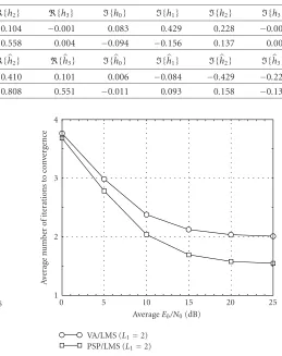
Table1: Shift ambiguity in estimated channel coefficients.
Actual channel coefficients {h0} {h1} {h2} {h3} {h0} {h1} {h2} {h3}
h1 −0.106 −0.410 −0.104 −0.001 0.083 0.429 0.228 −0.005
h2 −0.094 −0.809 −0.558 0.004 −0.094 −0.156 0.137 0.005
Estimated channel coefficients {h0} {h1} {h2} {h3} {h0} {h1} {h2} {h3}
h1 −0.011 0.105 0.410 0.101 0.006 −0.084 −0.429 −0.225
h2 0.000 0.101 0.808 0.551 −0.011 0.093 0.158 −0.136
100
10−1
10−2
10−3
10−4
0 5 10 15 20 25
Training-based scheme VA/LMS (L1=2)
PSP/LMS (L1=2) Known channel AverageEb/N0(dB)
Ra
w
b
it
er
ro
r
rat
e
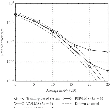
Figure3: Raw BER versus SNR for RA channel model.
(4) Final data estimate:steps (2) and (3) are repeated until
i= Niter or until a convergence of the estimated data sequence is observed, which gives the final data deci-sion.
4.4. Numerical results for uncoded transmission
The performance of the proposed blind sequence estima-tor was tested over a GSM-like system with burst length
K=148. At the transmitter, binary DPSK symbols are passed through a linearized Gaussian shaping filter, while a root-raised cosine filter is used as a receiving filter. The GSM05.05 rural area (RA) and typical urban (TU) channel models were taken into consideration. For the RA channel model, the memory length of channel model was fixed to be Lu = 2, while for the TU channel modelLu=3 was selected.
The problem of shift ambiguity is illustrated inTable 1 for the TU channel model. The estimated channel coeffi -cients are shifted to the right by one symbol (the phase ambiguity is uncritical due to differential encoding). Con-sequently, the estimated data sequences will be shifted by one symbol to the left compared to the transmitted data se-quences, that is, we have a BER of around 50% for such bursts. To eliminate this effect due to shift ambiguity, for the evaluation of the BER of uncoded systems we shift the
esti-4
3
2
1
0 5 10 15 20 25
VA/LMS (L1=2) PSP/LMS (L1=2)
AverageEb/N0(dB)
A
ver
age
n
umb
er
o
f
it
er
at
ions
to
con
ve
rgenc
e
Figure4: Average number of iterations of different algorithms to convergence for RA channel model,Niter=10.
mated data sequence by±Lusymbols and select the one with the lowest number of errors.
For comparison, simulation results were also shown for the case of known channel coefficients and a training-based scheme (where a GSM training sequence of length 26 is used for the LS channel estimation). The signal-to-noise ra-tio (SNR) loss due to the training sequence was taken into account. The final decision delay in all equalizers was se-lected to be 2(Lu+ 1). For the Viterbi equalizer in conjunc-tion with an LMS adaptive channel estimator (abbreviated as VA/LMS), the tentative decision delay is selected to be 5 sym-bols. The step size of LMS channel estimation is selected to be =0.1 in the first iteration for a fast convergence, while for remaining iterations it is chosen to be =0.01 for refine-ment of channel estimation. For SNRs < 20 dB, 104 quasi-static bursts were generated, that is, channel coefficients re-main constant within a burst and are statistically indepen-dent from burst to burst. For SNRs≥20 dB, the number of bursts is 105.
100
10−1
10−2
10−3
10−4
0 5 10 15 20 25
Training-based system VA/LMS (L1=3) PSP/LMS (L1=3)
PSP/LMS (L1=3) Known channel AverageEb/N0(dB)
Ra
w
b
it
er
ro
r
rat
e
Figure5: Raw BER versus SNR for TU channel model.
with a smaller complexity. For the TU channel model, as il-lustrated inFigure 5, all blind equalizers under investigation outperform the training-based system for SNRs≤15 dB. For PSP/LMS withLt =4, no error floor is visible. The gain of the PSP/LMS receiver withLt =4 is about 1 dB with respect to the training-based receiver, while the loss compared to the perfect channel knowledge is around 1 dB at the BER of 10−4. Similar to the RA channel model, a receiver with a higher complexity shows a faster convergence rate, as illustrated in Figure 6.
5. BLIND TURBO PROCESSOR
If a priori information about data symbols is available, we may apply a MAP sequence estimator for data estimation, that is, the branch metrics in the binary case are modified as [23,31]
γ˜x[k]
= −1
σ2 n
y[k]−
Lu
l=0
hl[k−1]˜x[k−l]
2
+ logPd˜[k]
= − 1
σ2 n
y[k]−
Lu
l=0
hl[k−1]˜x[k−l]
2
+1 2d˜[k]La
d[k],
(23)
whereLa(d[k]) is the given or estimated log-likelihood ra-tio value (abbreviated as L-value in the following) ofd[k]. (Symbol-by-symbol MAP estimation is not recommendable here due to the lack of survivors; surviving paths are neces-sary for channel estimation.)
5
4
3
2
1
0 5 10 15 20 25
VA/LMS (L1=3) PSP/LMS (L1=3) PSP/LMS (L1=4)
AverageEb/N0(dB)
A
ver
age
n
umb
er
o
f
it
er
at
ions
to
con
ve
rgenc
e
Figure6: Average number of iterations of different algorithms to convergence for TU channel model,Niter=10.
The significance of (23) is a generic receiver structure, which is the same for the full range of blind equalization without a priori information (where La(d[k]) = 0 for all
k) to a training-based equalizer (where|La(d[k])| → ∞for somek).
Besides incorporating a priori information, trellis-based blind equalizers are capable of delivering soft outputs to sub-sequent processing stages. Recently, blind turbo equalization techniques have been proposed in [37,38], where the chan-nel coefficients and the noise variance were estimated iter-atively using the off-line EM algorithm (compare (15) and (16)), and in [39], where a blind channel estimator based on higher-order statistics is used. The latter technique [39] has been investigated for fading channels. Our approach is suitable for short bursts, where the unknown channel co-efficients and data sequence are jointly estimated on the DPSK/ISI super-trellis. Moreover, the phase ambiguity and shift ambiguity problems are taken into consideration and solutions to combat such ambiguities are proposed, which may make our approach much more robust than related al-gorithms.
The overall system and the detailed turbo processor are illustrated in Figures7and8, respectively.
In Figure 7, u and d are the data vectors before and after channel encoding, respectively. Note that the “inner encoder” (represented by the DPSK/ISI super-trellis) is re-cursive, which is missing in the other blind turbo schemes [37,38,39], however.
Channel encoder
u d d
π Diencodingfferential channelISI Blind turboprocessor “Superchannel”
x y u
AWGN
Figure7: System model for blind turbo equalization.
SISO
blind equalizer π−1
SISO channel decoder π
LD
e(d)
LE e(d)
LE e(d)
LE e(d)
La(u) y
LD(u)
Figure8: Blind turbo processor.
In the following, we discuss the impacts of phase/shift ambiguity on the blind turbo processor, whileas novel ap-proaches are proposed to solve these problems. The max-log-APP algorithm is used in both the blind SISO equalizer and the SISO channel decoder. For convenience, we consider the binary case withLt=Luand assume that the estimated noise variance is equal to the true noise variance.
5.1. Estimated L-values under phase ambiguity
Ifh= −h, branch metrics in SISO blind equalizer is formu-lated as
γx˜[k]= −1
σ2 n
y(k) +
Lu
l=0
hlx˜[k−l]
2
+1 2La
d[k]d˜[k].
(24) For the nonblind case with known channel coefficients, branch metrics are evaluated as
γx˜[k]= − 1
σ2 n
y(k)−
Lu
l=0
hlx˜[k−l]
2
+1 2La
d[k]d˜[k].
(25) Comparing (24) with (25), we have
γx˜[k]=γ−x˜[k]. (26)
Given a symmetrical initialization for the forward recur-sion of the max-log-APP algorithm, that is, α(˜s[−1]) =
α(−˜s[−1]), it is easy to verify that
α˜s[k]=α−s˜[k], 0≤k≤K, (27)
where α(˜s[k]) = logp(yj≤k, ˜s[k] | h) and yj≤k = [y[0],
y[1],. . .,y[k]]T. Similarly, the backward recursion has the same property:
β˜s[k]=β−s˜[k], 0≤k≤K, (28)
whereβ(˜s[k])=logp(yj≥k+1 |˜s[k],h) andyj≥k+1 =[y[k+ 1],y[k+ 2],. . .,y[K]]T. Therefore, the approximated a
pos-teriori L-value ofd[k] can be obtained as
Ld[k]= max
˜
s[k]: ˜d[k]=+1
α˜s[k]+β˜s[k]
− max ˜
s[k]: ˜d[k]=−1
α˜s[k]+β˜s[k]
= max ˜
s[k]: ˜d[k]=+1
α˜s[k]+β˜s[k]
− max ˜
s[k]: ˜d[k]=−1
α˜s[k]+β˜s[k]
=Ld[k],
(29)
where ˜s[k] : ˜d[k] denotes all states consistent with ˜d[k]. Note that ˜s[k] and−˜s[k] will result in the same ˜d[k]. Hence, the correct L-values of data symbols are obtained under the con-ditionh= −h.
Moreover, the L-value about the reference symbol must be estimated rather than assumed to be known. Otherwise, the L-value about the first data symbol is evaluated as follows:
Ld[1]|x[0]=+1 = max
˜
d[1]=x˜[1]=+1
α˜s[1]+β˜s[1]
− max ˜
d[1]=x˜[1]=−1
α˜s[1]+β˜s[1]
= max ˜
d[1]=x˜[1]=−1
α˜s[1]+β˜s[1]
− max ˜
d[1]=x˜[1]=+1
α˜s[1]+β˜s[1]
= −Ld[1].
(30)
If L(d[1]) obtained in (30) is delivered to the channel de-coder, it will cause error propagation during the iterative pro-cessing.
5.2. Shift ambiguity compensation
For a possible shift to the right in the channel estimation, we have
hl=hl−κ, κ≤l≤L+κ,
hl=0, l < κorL+κ < l≤Lu,
(31)
u
ENCo co Πo c o
S/P co,1
co,N . . .
ci,1
ci,N
Πi,1 Πi,N ENCi,1
ENCi,N
d1
dN
CHA1 CHAN
EQUN EQU1
Le(dN)
Le(d1)
L(co,N)
Le(co,1)
. . . P/S
Le(co)
Le(co)
L(u)
SC moduleN SC module1 Π−1
o DECo
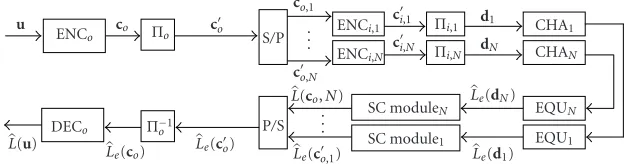
Figure9: Proposed transmitter/receiver structure for fading channels.
We consider the very first iteration between the blind SISO equalizer and the SISO channel decoder, where no a priori information about d[k] is available. Branch metrics under shifted channel coefficients are then formulated as
γx˜[k]= −1
σ2 n
y[k]−
Lu
l=0
hlx˜[k−l]
2
= −1
σ2 n
y[k]−
L
l=0
hlx˜[k−κ−l]
2
.
(32)
For the case with correct channel coefficients, branch metrics are evaluated as follows:
γx˜[k]= − 1
σ2 n
y[k]−
L
l=0
hlx˜[k−l]
2
. (33)
By means of induction, the estimated L-values can be ob-tained as
Ld[k]= max
˜
x[k]: ˜d[k]=+1
α˜s[k]+β˜s[k]
− max ˜
x[k]: ˜d[k]=−1
α˜s[k]+β˜s[k]
=Ld[k+κ],
(34)
that is, the estimated L-values of shifted channel coefficients are shifted in the reverse direction, see (31). This argument is verified in the appendix.
Because of the deinterleaver between the SISO equalizer and the SISO channel decoder (cf. Figure 8), a valid code-word is not valid any more after shifts, that is, only the L-values corresponding to the correct shift index will give rea-sonable soft outputs of the channel decoder. Based on this fact and on (34), we propose to shift the estimated L-values obtained from the SISO blind equalizer. Then the shift index can be estimated as
κ=arg max m
KR
n=1
1
KRL
D(m)u[n]
, (35)
where L-values about uncoded symbols related to shiftsm∈ [−LM,LM] are denoted as{|LD(m)(u[n])|}andLM≤Lu con-trols the range of shift search. Moreover,Rdenotes the code rate of the channel encoder andKRis assumed to be a pos-itive integer. In the following, (35) is referred to as a shift compensation module (SC module).
5.3. Double serial concatenation for fading channels
Conventionally, for frequency-hopping systems over fading channels, an interburst interleaver is used in conjunction with a channel encoder in order to explore the time diversity of the channel code. On average, within severely faded bursts the L-values of the coded symbols have significantly smaller magnitudes than in nonfaded bursts. After deinterleaving, the L-values with small magnitudes are spread over the whole coded block. Therefore, it is easy to compensate these small L-values with the help of their “neighbors” with relatively large magnitudes. For blind turbo equalizers, a direct ap-plication of interburst interleaving isnot straightforward be-cause of the shift ambiguity problem. In order to combat the shift ambiguity associated with individual bursts, the shift ambiguity compensation should be carried out for individ-ual bursts rather than for the whole coded block. Therefore, channel encoding is applied for individual bursts as shown in Figure 7, while the shift compensation is performed as pre-sented inSection 5.2for individual bursts. Moreover, a fur-ther outer channel encoder is introduced to exploit time di-versity in conjunction with inter burst interleaving, similarly as in the conventional case with known channel coefficients. This new scheme, which has a double serially concatenated structure, is illustrated inFigure 9.
After the outer interleaver, denoted asΠo, the coded data symbols from the outer channel encoder ENCo(with a code rate of Ro) are divided intoN parallel substreams co,l, 1 ≤
the estimated L-values about its infobitsL(u) and also deliv-ers the estimated a priori information for the inner channel decoders in the next iteration.
Because it is difficult to optimize the double serially con-catenated system, the whole system is intuitively designed to get a compromise between the complexity and performance. Both inner and outer channel codes should be strong codes for a large time diversity and a reliable shift compensation, respectively. Within this paper, we consider rate 1/2 convolu-tional codes, where “strong code” means a sufficiently large memory length. On the other hand, to avoid a low bandwidth efficiency, we need a punctured code [40]. Therefore, a rea-sonable choice is to select an unpunctured code with a short memory length for the outer concatenation and a punctured code with a long memory length for the inner concatenation.
5.4. Overall receiver
Two scheduling strategies are possible: iterative processing between the SISO modules may be performed after a con-vergence of the TABSE (the receiver based on this scheduling strategy is referred to as Scheme 1), or the iterative process-ing is carried out directly after the all-zero initialization (the corresponding receiver is referred to as Scheme 2). Scheme 2 requires more iterations than Scheme 1 to achieve a similar performance, because in Scheme 1 the quality of soft out-puts from the SISO blind equalizer are more reliable than in Scheme 2 at least at the initial phase of iterative processing. Therefore, within this paper, we only consider Scheme 1.
The overall receiver for coded systems in thejth iteration is described as follows.
(1) Soft-output equalization:the forward recursion is per-formed by means of adaptive joint data/channel es-timation, where the branch metrics are evaluated as in (23). The backward recursion is carried out using the transition probabilities obtained in the forward re-cursion. Afterward, the L-values about data symbols before the differential encoding are evaluated to get {LE
e(d[k])}.
(2) Noise variance estimation: after the evaluation of L-values of coded data symbols, the noise variance can be estimated based on hard or soft decisions from the SISO equalizer, refer to (16) and (19), respectively. The estimated noise variance is used in the next iteration to evaluate the branch metrics (cf. (23)).
(3) SISO channel decoding of inner codes:the branch met-rics inlth (1≤l≤N) SISO inner channel decoder are calculated as (0≤n≤KRi,l−1)
γ(j)˜c
i,l[n]
=
(n+1)/Ri,l−1
k=n/Ri,l
L(ej)
ci,l[k]
˜
ci,l[k]
+ L(aj−1)co,l[n]
˜
co,l[n],
(36)
where ˜ci,l[n] = [˜ci,l[n/Ri,l],. . ., ˜ci,l[(n+ 1)/Ri,l−1]]T is the inner coded data symbol vector at index n
and{L(ej)(ci,l[k])}are extrinsic information obtained from thelth SISO equalizer. Moreover,L(aj−1)(co,l[n])
denotes the estimated a priori information about coded bitsco,l[n] of outer code (i.e., info-bits of inner codes) from the outer channel decoder in the (j−1)th iteration. The extrinsic information about coded bits {ci,l[k]} obtained by the max-log-APP channel de-coder is fed back to thelth SISO equalizer and used as estimated a priori information in the next iteration. The extrinsic information about info-bits{co,l[k]}is passed to the outer channel decoder after the parallel-to-serial converter. Only in the very first iteration, the possible shift ambiguity in the SISO equalizer is compensated by means of the proposed approach (cf. Section 5.2). L-values corresponding to the optimal shift index are delivered to the inner SISO channel de-coders.
(4) SISO channel decoding of outer code:the branch met-rics in the SISO outer channel decoder are calculated as (0≤n≤KNl=1Ri,l·R0−1)
γ(j)˜c
o[n]
=
(n+1)/Ro−1
k=n/Ro
L(ej)co[k]
˜
co[k]
+ La
u[n]u˜[n],
(37)
where ˜co[n] = [co[n/Ro],. . .,co[(n+ 1)/Ro−1]]T is the outer coded data symbol vector and{L(ej)(co[k])} are extrinsic information from the inner channel de-coders. Moreover,La(u[n]) denotes the available a pri-ori information about info-bitsu[n] of outer code. (5) Final data estimation:steps (1)–(4) are repeated until
the given number of iterations is reached. The L-values from the outer channel decoderL(u) deliver the hard decisions about info-bits and their corresponding reli-abilities.
5.5. Numerical results for coded systems
Simulations were performed for the quasi-static TU and RA channel models using the proposed double serially concate-nated scheme. The outer channel encoder is a rateR0 =1/2 convolutional code with generator polynomials (5, 7). The inner codes (N=10) are recursive systematic convolutional codes with the same generator polynomials (23, 35), which are punctured to get a code rate ofRi,l = 2/3, 1 ≤ l ≤ 10. The puncturing table is [1111, 0101], where 0 stands for the puncturing. Accordingly, the overall code rate is 1/3. No zero tailing or tail biting is applied. The code length of the outer code is 1000, while the inner codes have a code length of 150.
100
10−1
10−2
10−3
10−4
10−5
0 2 4 6 8 10 12 14 16
1 iter. 2 iter. 3 iter.
5 iter. 7 iter. AverageEb/N0(dB)
Bi
t
er
ror
ra
te
Figure 10: BER versus SNR of coded schemes for RA channel model. Solid lines and dashed lines correspond to simulation results of blind schemes and schemes with perfect channel knowledge, re-spectively.
100
10−1
10−2
10−3
10−4
10−5
0 2 4 6 8 10 12 14 16
1 iter. 2 iter. 3 iter.
5 iter. 7 iter. AverageEb/N0(dB)
Bi
t
er
ror
ra
te
Figure 11: BER versus SNR of coded schemes for TU channel model. Solid lines and dashed lines correspond to simulation results of blind schemes and schemes with perfect channel knowledge, re-spectively.
As shown in Figures 10 and 11, for the systems with perfect channel knowledge (known channel coefficients and known average SNRs), the first iteration between the SISO equalizer and SISO channel decoders provides the most sig-nificant improvement. There is no further improvement af-ter about 3 iaf-terations for the considered SNR region. For
100
10−1
10−2
10−3
0 2 4 6 8 10 12 14 16
1 iter. 2 iter. 3 iter.
5 iter. 7 iter. AverageEb/N0(dB)
MSE
o
f
channel
co
e
ffi
cie
n
ts
estimatio
n
Figure 12: MSE of estimated channel coefficients versus average
Eb/N0for different iterations, for RA channel model.
100
10−1
10−2
10−3
0 2 4 6 8 10 12 14 16
1 iter. 2 iter. 3 iter.
5 iter. 7 iter. AverageEb/N0(dB)
MSE
o
f
channel
coe
ffi
cie
n
ts
estimatio
n
Figure 13: Decreased MSE of estimated channel coefficients through the iterative processing, for TU channel model.
6. CONCLUSIONS
Based on an approximation of a blind maximum-likelihood sequence estimator, reduced-complexity iterative adaptive trellis-based blind sequence estimators are proposed. Previ-ously proposed blind sequence estimators can be interpreted as special cases of our proposed receiver. Moreover, the ideas of PSP/PBP are generalized by replacing conventional branch metrics by short-path metrics. The differential encoder (or generalizations thereof) is used to combat the phase ambi-guity, where the resulting DPSK/ISI super-trellis is explicitly applied for SISO equalization. By means of (de-)interleaver and channel encoder, the problem of shift ambiguity due to the overdetermined channel order can be resolved efficiently. For frequency-hopping systems over frequency-selective fad-ing channels, a double serially concatenated scheme is pro-posed, which can combat the shift ambiguity and explore the time diversity of channel codes in conjunction with inter-burst interleaving. Our simulation results demonstrate the potential of trellis-based adaptive blind sequence estimators for short-burst data transmission over practical fading chan-nels, particularly in the presence of channel coding.
APPENDIX
A. L-VALUES UNDER SHIFT AMBIGUITY
In this appendix, we consider the relationship between L-values conditioned on shifted channel coefficients and cor-rect L-values. The following conditions are presumed:
hl=hl−κ, κ≤l≤L+κ,
hl=0, l < κorL+κ < l≤Lu,
γx˜[k]= −1
σ2 n
y[k]−
L
l=0
hlx˜[k−κ−l]
2
,
γx˜[k]= −1
σ2 n
y[k]−
L
l=0
hlx˜[k−l]
2
,
(A.1)
and the max-log-APP algorithm is employed.
A.1. Definitions
Firstly, we introduce some relevant definitions.
(i) A state at the time index k, which merges into the states[k+κ] afterκsteps in the forward recursion, is called a forward-consistent state of s[k+κ]. The set of forward-consistent states ofs[k+κ] at time indexkis termed forward-consistent state setofs[k+κ] and abbreviated asMk (s[k+κ]). Similarly, a state at time index k + κ, which merges into the state s[k] afterκsteps in the backward recursion, is termed a backward-consistent state of s[k]. The set of backward-consistent states of s[k] at time index k +κ is termedbackward-consistent state setofs[k] and abbreviated asMk +κ(s[k]).
(ii) A state transition at time indexk,x[k], which con-nects two forward-consistent states of s[k+κ], is called a forward-consistent state transition ofs[k+κ]. The
forward-consistent transition setofs[k+κ] at time indexkis abbrevi-ated asQk (s[k+κ]).
Similarly, a state transition at time indexk+κ, which connects two backward-consistent states of s[k], is called a backward-consistent state transition of s[k]. The backward-consistent transition setofs[k] at time indexk+κis referred to asQk +κ(s[k]).
(iii) A state s1[k] = [x1[k −Lu + 1],. . .,x1[k]]T is
κ-equivalent to another state s2[k] = [x2[k − Lu + 1],
. . .,x2[k]]T, ifx1[k−κ−l]=x2[k−κ−l], 0≤l≤L(for the caseLu> κ+L), or ifx1[k−κ−l]=x2[k−κ−l], 0≤l≤L−1 (for the caseLu=κ+L). A states1[k] isκ-shift equivalentto another states2[k], ifx1[k−κ−l]=x2[k−l], 0≤l≤L(for the caseLu> κ+L), or ifx1[k−κ−l]=x2[k−l], 0≤l≤L−1 (for the caseLu=κ+L).
A state transitionx1[k] =[x1[k−Lu],. . .,x1[k]]T isκ -equivalent to another state transitionx2[k] = [x2[k−Lu],
. . .,x2[k]]T, if x1[k−κ−l] = x2[k−κ−l], 0 ≤ l ≤ L. A state transitionx1[k] isκ-shift equivalentto another state transitionx2[k], ifx1[k−κ−l]=x2[k−l], 0≤l≤L.
(iv) For the forward recursion, we define
s[k]−xk−Lu+ 1
,xk−Lu+ 2
,. . .,x[k]T,
ifs[k]=xk−Lu+ 1
,xk−Lu+ 2
,. . .,x[k]T,
x[k]−xk−Lu
,xk−Lu+ 1
,. . .,x[k]T,
ifx[k]=xk−Lu
,xk−Lu+ 1
,. . .,x[k]T.
(A.2)
Correspondingly, for the backward recursion, we define
s[k]xk−Lu+ 1
,. . .,x[k−1],−x[k]T,
ifs[k]=xk−Lu+ 1
,. . .,x[k−1],x[k]T,
x[k]xk−Lu
,. . .,x[k−1],−x[k]T,
ifx[k]=xk−Lu
,. . .,x[k−1],x[k]T.
(A.3)
(v) For the evaluation of L-values under correct chan-nel coefficients, the relevant state transitions are defined as
xr[k][x[k−L],. . .,x[k]]T. Accordingly,xr[k][−x[k−
L],. . .,x[k]]T. The relevant states are defined as s
r[k]
[x[k−L+ 1],. . .,x[k]]T (for the caseL
u=L+κ) or defined assr[k] [x[k−L],. . .,x[k]]T (for the caseLu > L+κ). Accordingly,sr[k][−x[k−L+ 1],. . .,x[k]]T(for the case
Lu=L+κ) andsr[k][−x[k−L],. . .,x[k]]T(for the case
Lu> L+κ).
A states1[k]=[x1[k−Lu+ 1],. . .,x1[k]]T is relevant-equivalent to another state s2[k] = [x2[k − Lu + 1],
. . .,x2[k]]T, ifx1[k−l]=x2[k−l], 0≤l≤L.
A.2. L-values under shifted channel coefficients
In the following, only the caseLu=L+κis considered, while the extension toLu> L+κis straightforward.
Theorem 1. Ifs1[k]and s2[k] areκ-equivalent states, then