Multivariate Quadratic Problems
⋆Takanori Yasuda1, Xavier Dahan1,6, Yun-Ju Huang1,2, Tsuyoshi Takagi1,3,4, and Kouichi Sakurai1,5
1 Institute of Systems, Information Technologies and Nanotechnologies
2
Graduate school of Mathematics, Kyushu University 3 CREST, Japan Science and Technology Agency
4
Institute of Mathematics for Industry, Kyushu University 5 Department of Informatics, Kyushu University
6
Leading Graduate School Promotion Center, Ochanomizu University
Abstract. Multivariate Quadratic polynomial (MQ) problem serve as the basis of security for potentially post-quantum cryptosystems. The hardness of solving MQ problem depends on a number of parameters, most importantly the number of variables and the degree of the polynomials, as well as the number of equations, the size of the base field etc. We investigate the relation among these parameters and the hardness of solving MQ problem, in order to construct hard instances of MQ problem. These instances are used to create a challenge, which may be helpful in determining appropriate parameters for multivariate public key cryptosystems, and stimulate further the research in solving MQ problem.
Keywords: Post-quantum cryptography, Multivariate public-key cryptosystems, Gr¨obner basis
1
Introduction
Multivariate public-key cryptosystems [14, 33] (MPKC for short) are candidates for post-quantum cryptography. MPKC are schemes that use multivariate polynomial maps as public keys. The security of MPKC is thus based on the one-wayness of the multivariate polynomial maps. In the same vein, QUAD [4] is a stream cipher (symmetric key cryptography) whose security is guaranteed by the one-wayness of the multivariate polynomial maps.
The one-wayness of multivariate polynomial maps resides in the difficulty to find solutions of a system of multivariate polynomial equations (MP problem). In particular, if the multivariate polynomials involved in a MP problem consist only of quadratic polynomials, the problem is called MQ problem:
f1(x1, . . . , xn) = ∑
1≤i≤j≤n
a(1)ij xixj+ ∑
1≤i≤n
b(1)i xi+c(1)=d1,
f2(x1, . . . , xn) = ∑
1≤i≤j≤n
a(2)ij xixj+ ∑
1≤i≤n
b(2)i xi+c(2)=d2,
.. .
fm(x1, . . . , xn) = ∑
1≤i≤j≤n
a(m)ij xixj+ ∑
1≤i≤n
b(m)i xi+c(m)=dm,
⋆
where m is the number of equations, n the number of variables, and a(1)ij , b(1)i , c(1), . . . are all elements in a finite fieldF.
Since many schemes in MPKC make use only of quadratic polynomials, the analysis for solving MQ problems is important. In this paper, we present a sequence of MQ problems of different level of difficulty, which we propose as a world wide challenge. The construction of these MQ problems is based both on theoretical and on practical considerations.
MPKC can be used both in encryption schemes and in signature schemes. The original idea of MPKC was presented by Matsumoto and Imai [26], and their scheme is commonly referred to as theMI scheme. After MI scheme was proposed, several encryption systems were proposed such as HFE [28] andℓ-IC [17]. Unfortunately, most of them including MI, HFE andℓ-IC were broken after several security analyses [27, 24, 22]. Nonetheless, recently, two new encryption schemes have been proposed. First, the “simple matrix” scheme (ABC scheme) [32] which was presented at PQCrypto 2013 is an encryption scheme using matrix operations whose components consist of elements in a finite field of small size. An enhanced extension of this scheme was proposed at PQCrypto 2014 [16]. Second, the ZHFE scheme [30], also proposed at PQCrypto 2014, is an enhancement of the HFE scheme.
On the other hand, UOV [23] is a signature scheme using polynomials with a distinction on the variables into two kinds: oil variables and vinegar variables. Rainbow [15] is the “multilayered version” scheme of UOV. The framework of Rainbow, using (commutative) polynomial rings, has been extended to non-commutative rings. The security of this scheme was analyzed in [35]. The structure of the associated MQ problems for encryption schemes and signature schemes are substantially different. For encryption schemes, the associated MQ problem verifies m≥n (overdetermined), while for signature schemes, the associated MQ problem hasm≤n (underde-termined). Therefore, we must prepare difficult problems of two kindse.g.whenm≥nand when m ≤n. In addition, we distinguish finite fieldsF of characteristic 2 and of odd characteristic, regarding that the approach to solve the MQ problems is quite different.
On the other hand, the specificity of MQ problem over GF(2) has attracted the attention of several researchers in cryptography. Concerning signatures, in the extended version of [28], Patarin introduced two HFE challenges (coming with a prize of US $ 500 for attacking any of them). HFE challenges include MQ problems over GF(2) saw many researchers trying to solve the problems [13]. Moreover, the solving technique of MQ problem is also applied to other cryptography. The technique is used to the security analysis of the block cipher [12]. Therefore, our instances of MQ problem include those overGF(2).
When creating challenge, one of the most important matter is to guarantee the fairness of challenging problem. We mean here that the problem is evenly difficult for anybody, including the creator himself. ECC challenge [18] and Lattice challenge [25] have been built in this way. Indeed, instances of elliptic curve discrete logarithm problems and short vector problems can be created without knowing the solution. However, this is not the case for the RSA challenge [31]. Generating a composite number without knowing its factors is indeed difficult. Therefore, RSA challenge may become an unfair contest. It is also difficult to create MQ problem without knowing a solution in advance. However, we want to create MQ problem whose fairness is guaranteed. In order to achieve this, we considered two strategies. One is the use of systems of equations with completely random coefficients. Generally, these systems may not have solutions. However, the underdetermined systems have at least one solution with high probability. Another is a construction from a random solution. For the overdetermined systems, we use this method.
precisely as possible. We have experimented solving several MQ problems with small parameters, and by combining the theoretical complexity bounds involving the degree of regularity, we have extrapolated the results of these experiments to create hard instances of MQ problems.
2
Fundamental Structure of MPKC
In both cases of encryption and of signature under MPKC, a multivariate quadratic polynomial map whose inverse map can be computed easily is required. Such a polynomial map is called a central map. Given a central map G: Kn → Km, a multivariate quadratic polynomial map F : Kn → Km of the form F = L◦G◦R can be constructed by where L and R are affine transformations onKmandKn, respectively. For a person who does not know the central map G, nor the two affine transformationsL, R, the mapF must look like a multivariate quadratic polynomial map chosen randomly. If so, F plays the role of a trapdoor one-way function, and thus would be the public key. The private key would consist of the central mapGand of the affine transformations Land R. Hereafter in this section, we review in more details MPKC schemes, with the distinction encryption/signature.
2.1 Encryption Case
From the feature of an encryption scheme,Gand F both must be (almost) injective. This fact imposes that m ≥ n. For example ABC scheme and ZHFE scheme both use parameters such that m= 2n. Encryption and decryption are described as follows:
Encryption A plain textM is selected fromKn. An encryptor computesC =F(M) ∈Km. This is the associated cipher text.
Decryption The decryptor computes E1 = L−1(C), E2 = G−1(E1), E = R−1(E2) in this order. Then Ecoincides with M.
2.2 Signature Case
From the feature of a signature scheme, Gand F both must be surjective. This fact imposes that m ≤ n. UOV and Rainbow satisfy this property. UOV often uses parameters such that n= 2m, justified by security reasons. For Rainbow, the recommended parameters are estimated in [29] andn≈1.5m is considered to be suitable for Rainbow. In a signature scheme, signature generation and verification are performed as follows:
Signature generationA messageM is selected fromKm. The signer computesS
1=L−1(M), S2=G−1(S1),S =R−1(S2) in this order. ThenS is the associated signature.
Verification A verifier computes F(S) ∈ Km, and checks if M = F(S), in which case The signature is accepted.
3
General Attack against MQ Problem
Let Fq denote the finite field of order q and Fq[x1, . . . , xn] the polynomial ring over Fq with n variables. For any f = (f1(x1, . . . , xn), . . . , fm(x1, . . . , xn)) ∈ Fq[x1, . . . , xn]m, MP problem indicates the following computational hard problem:
Question: find a common zerox0∈Fnq of the polynomialsf1, . . . , fm.
If the degree of all f1, . . . , fm are equal to 2, the corresponding MP problem is calledMQ
3.1 Complexity of F5 Algorithm
Definition 1. Let (h1, . . . , hm) ∈ Fq[x1, . . . , xn]m be homogeneous polynomials. The degree of
regularity of a homogeneous idealI =⟨h1, . . . , hm⟩is defined by
dreg = min {
d≥0dimFq({f ∈ I,deg(f) =d}) = (
n+d−1 d
)} .
For non-homogeneous polynomials (f1, . . . , fm) ∈ Fq[x1, . . . , xn]m, the degree of regularity is
defined by that of the ideal⟨f1h, . . . , fm⟩h , wherefihis the homogeneous part offi of highest degree.
Note that in this last case, it is not an invariant of the ideal, but is attached to the polynomial system.
For a MQ problem with zero dimensional solution variety, the complexity ofF5 algorithm is given by the following.
Proposition 1. [2] The complexity of computing a Gr¨obner basis of a zero-dimensional system of mequations inn variables withF5 is:
O ((
m· (
n+dreg−1 dreg
))ω)
wheredreg is the degree of regularity of the system and2≤ω≤3 is the linear algebra constant. Recall that random underdetermined systems are regular. The concept of semi-regularity was introduced to formalize “random systems”, in the case of overdetermined systems. (though this fact is not proven in general, theFr¨oberg’s conjecturehas been widely observed in practice).
Definition 2. Let (h1, . . . , hm)∈Fq[x1, . . . , xn]mbe homogeneous polynomials of respective
de-gree d1, . . . , dm. This sequence is semi-regular if – ⟨h1, . . . , hm⟩ ̸=Fq[x1, . . . , xn],
– for all1≤i≤m andg∈Fq[x1, . . . , xn],
deg(g·hi)< dreg andg·hi∈ ⟨h1, . . . , hi−1⟩ ⇒g∈ ⟨h1, . . . , hi−1⟩.
For a general system(f1, . . . , fm)∈Fq[x1, . . . , xn]m, this sequence issemi-regularif the sequence (f1h, . . . , fmh)is, where fih is the homogeneous part offi of highest degree.
The degree of regularity of semi-regular sequences can be computed explicitly.
Proposition 2. The degree of regularity of a semi-regular sequence h1, . . . , hmof respective
de-gree d1, . . . , dm is given by the first non-positive coefficient of ∑
k≥0 ckzk=
∏m i=1(1−z
di)
(1−z)n .
3.2 Complexity of Hybrid Approach
Concerning systems of dimension zero defined over a finite field of medium size, the hybrid approach consists in choosing k variables, evaluate them at randomly chosen values, and solve this system in n−k variables. The choice of k is delicate, but when making some reasonable assumptions (see Hypothesis 1 below), the authors of [2] succeed to provide a theoretical opti-mal choice of k depending of the data of the system. This outcome allows them to apply this hybrid approach to forge signatures based on a MPKC scheme (namely TMRS and UOV signa-tures, see [11, Section 4.1 & 4.2]) by solving underdetermined systems, where traditional solving approaches failed.
Despite we have not put into practice this approach in the experiments, we have followed the same strategy to solve underdetermined systems (Type IV,V,VI): evaluation ofm−nvariables to reduce to a zero-dimensional systems. To solve the zero-dimensional system, we have used a standard approach rather than the hybrid, which we plan to do in the future.
Proposition 3. For f = (f1(x1, . . . , xn), . . . , fm(x1, . . . , xn))∈ Fq[x1, . . . , xn]m, let dreg(k) be
the maximum degree of regularity of all the systems:
{
{f1(x1, . . . , xn−k, v1, . . . , vk), . . . , fm(x1, . . . , xn−k, v1, . . . , vk)} |(v1, . . . , vk)∈Fkq }
If the system is zero-dimensional, the complexity of the hybrid approach is bounded from above by
O (
min0≤k≤n {
qk· (
mω· (
n−k+dreg(k)−1 dreg(k)
)ω
+ (n−k)d(n−k)ω )})
where2≤ω≤3.
The optimal choice ofkis usually small from 1 to 4 or 5 for common MQ problems. If the base field isGF(2), it is better to add the field equations to the system than to resort to the hybrid approach.
In order to grasp the asymptotic behavior of the hybrid approach, we assume a regularity condition set in [2].
Hypothesis 1 Let {f1, . . . , fm} ⊂ Fq[x1, . . . , xn] be polynomials of respective degrees d1 ≥ · · · ≥ dm. Letβmin, 0 < βmin <1 be a value that will be specified later. Then, for any k, 0≤k≤ ⌈βminn⌉, and for each vector (v1, . . . , vm)∈Fkq, the system,
{
{f1(x1, . . . , xn−k, v1, . . . , vk), . . . , fm(x1, . . . , xn−k, v1, . . . , vk)} |(v1, . . . , vk)∈Fkq }
is semi-regular fornlarge enough.
4
Construction of the Challenge
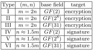
We explain how to create MQ problems. The parameters that need to be set for a MQ problem are the size of base fieldq, the number of variablesnand the number of equationsm. As for base fields, we treatGF(2) as a special case. Otherwise we considerGF(31) and GF(28) because the situation changes according to whether the characteristic of the base field is two or not. These two fields are often used as base fields in many papers [9, 29].
are used because the associated multivariate polynomial functions have to be surjective. Since Rainbow is a signature scheme which enhances UOV, we treat Rainbow as a representative of signature scheme in MPKC. In the case of Rainbow with 2 layers, number of polynomialsmand of variablesnare often set ton≈1.5m. Therefore, in our challenge, we set problems of six types, described in Table 1
Table 1.Types of MQ problem
Type (m, n) base field target I m= 2n GF(2) encryption II m= 2n GF(28) encryption III m= 2n GF(31) encryption IV n≈1.5m GF(2) signature
V n≈1.5m GF(28) signature VI n≈1.5m GF(31) signature
We consider two construction methods of MQ problem. One is for encryption and another is for signature. For encryption,m≥n, however, for every systemm > n, the probability is about
1
qm−n to have a solution, and if we setm=n, it is the case which had the same time complexity
with the signature case. Therefore, we construct the system corresponding to encryption scheme with a random solution by adjusting the constant coefficients. For the signature case, we construct the system with all random coefficients.
Algorithm 1: Construction of MQ problem for type I, II, III
Step 1 Fix parametersnandm= 2nwith base field overF =GF(2), GF(28) orGF(31). Step 2 Select randomly a vectorx0in Fn.
Step 3 Select randomlya(k)ij , b(k)i for alli, j, k.
Step 4 Computec(k) such that the associated system of equations has a solutionx 0.
Algorithm 2: Construction of MQ problem for type IV, V, VI
Step 1 Fix parametersmandn= 1.5mwith base field overF =GF(2), GF(28) orGF(31). Step 2 Select randomlya(k)ij , b(k)i , c(k) for alli, j, k.
5
Experiments
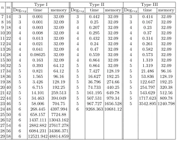
Table 2.Experimental results of Type I, Type II and Type III
n m Type I Type II Type III
Degreg time memory Degreg time memory Degreg time memory
7 14 3 0.001 32.09 3 0.442 32.09 3 0.414 32.09
8 16 3 0.001 32.09 3 0.25 32.09 3 0.167 32.09
9 18 4 0.003 32.09 4 0.207 32.09 4 0.23 32.09
10 20 4 0.008 32.09 4 0.295 32.09 4 0.37 32.09
11 22 4 0.013 32.09 4 0.432 32.09 4 0.314 32.09
12 24 4 0.021 32.09 4 0.24 32.09 4 0.261 32.09
13 26 4 0.041 32.09 4 0.47 32.09 4 0.582 32.09
14 28 4 0.08625 32.09 4 0.559 32.09 4 0.573 32.09
15 30 4 0.163 32.09 4 0.864 32.09 4 1.319 32.09
16 32 5 0.393 64.12 5 0.864 32.09 5 1.319 32.09
17 34 5 0.821 64.12 5 7.427 128.19 5 21.486 96.16
18 36 5 1.565 96.16 5 16.627 192.25 5 53.836 128.19 19 38 5 3.426 128.19 5 36.796 274.66 5 122.647 192.25 20 40 5 6.715 192.25 5 74.733 440.25 5 254.797 320.38 21 42 5 14.101 259.513 5 161.195 649.78 5 543.629 512.56 22 44 5 34.463 394.049 5 507.531 979.34 5 1717.623 809.78 23 46 5 58.006 704.75 5 967.727 1656.528 5 3542.895 1240.798 24 48 6 268.445 4397.994 6 9268.363 10681.12
25 50 6 658.157 7724.88 26 52 6 1437.111 13043.162 27 54 6 2882.882 27617.278 28 56 6 6084.231 34366.371 29 58 6 12521.942 48814.859
Table 3.Experimental results of Type IV, Type V and Type VI
n m Type IV Type V Type VI
Degreg time memory Degreg time memory Degreg time memory
11 7 8 1.261 32.09 9 2.597 32.09 9 1.981 32.09
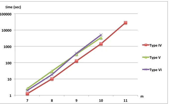
Fig. 1.Time comparison for Type I, II, and III
applied here were only toy example, and the total time of the experiments would not exceed one week.
For every experiment, we generated a random multivariate quadratic system with coefficients in random uniform distribution with specific format. The input format is described in the Ap-pendix. Then we read the input file and solve the system usingVariety() function of Magma.
Table 2 shows the experimental results of Type I, Type II and Type III. Degregrepresents the degree of regularity, which indicates the largest degree appeared during the process of computing a Gr¨obner basis. In this case, we simulate an encryption scheme without knowing any structure of it. Since in this case the system is overdetermined, we adjust the constant coefficients to make sure that the system has a solution. Actually for an overdetermined system, even if m=n+ 1, the probability to have a solution is quite small. Let the number of variables to be n, the number of equations to bem, the size of the coefficient field to beq, then the probability of an overdetermined system to have a solution is roughly qm1−n. For systems of Type I, defined over
the binary field, we add the field equations to the system.
Table 3 shows the experimental results of Type IV, Type V and Type VI. In this case, we simulate an signature scheme without knowing any structure of it. Note that in this case, since n = 1.5m, there are more free variables in the MQ system than the equations and thus the system is underdetermined. Generally when we solve such system, we assign random values to the free variables and solve the remained determined system. We use this technique here. Hence, the system may have the same time complexity and degree of regularity with that of the system n=m. For systems of Type IV, defined over the binary field, we add the field equations to the system.
Fig. 1 and Fig. 2 show the time comparison for the encryption case and the signature case respectively. Note that the x-axis indicates the number of variablesn for systems of type I, II and III, whereas it indicates the number of equationsm for systems of type IV, V and VI.
6
The Challenge
In Section 4, we explained the method for constructing the MQ challenge, which was used in Section 5 to construct toy examples of MQ problems. The timings obtained on these toy examples serve an experimental basis to determine parameters yielding harder instances of MQ systems, and which would require at least a month to be solved. More precisely, at least one month when equipped with a similar computational environment described in the beginning of Section 5, and using “plain” techniques (but possibly adapted to the different six Types of systems). This is because the systems are essentially random.
This challenge does not include MQ systems which aresparse. However, sparse systems form an important class of MQ problems, since it provides more efficiency for encryption and verifi-cation of MPKC. We plan to include this kind of challenge in the future.
In creating MQ challenges, we choose starting values of parametersm, nsuch that the time required for solving systems with the same parameters (extrapolation) exceeds a month.
Table 4.Minimum ofmandn
Type I II III IV V VI
(m, n) (110,55) (70,35) (68,34) (55,82) (16,24) (16,24)
exhaustive search by using the result of the benchmarks displayed in the homepage of libFES. According to this estimation, we have that when n = 55 and m = 110 in Type I case, the exhaustive search takes about a month. On the other hand, in our experiment, whenn= 35 and m= 70, the estimation given by Gr¨obner basis computation is also about a month. Comparing our experiments to the estimation of libFES, leads to the following conclusion: for a fixed couple (m, n), the of Gr¨obner basis computation time becomes about 1,000,000 times that of libFES exhaustive search. In Type IV case, parametersm, nare set such thatn= 1.5m. If we substitute random values to a number of variables equal to 1.5m−m= 0.5m, this MQ problem of Type IV can be reduced to MQ problem of square type. By using the result of libFES, we can estimate that when n= 82 andm= 55 in Type IV case, the exhaustive search takes about a month.
Next consider the case of base field equal toGF(28) and toGF(31). Form, nof small sizes, the XL method is effective against MQ problems, as well as is the Hybrid approach. The paper [10] presents experimental results of the XL method. We make use of these results and of our experiments of type II, III, V and VI to estimate the starting parameters of MQ challenges. If we try to solve MQ problem using the Hybrid approach, it is necessary to estimate a suitable number of variables for substitution. According to theoretical computation of the paper [2], in practice this number is rarely larger than two. Therefore we choose (m, n) as starting parameter of MQ challenges such that the time for solving the MQ problem with (m−2, n−3) using Magma F4 algorithm is over a month. From the experiments of Type II and III, the gradient of the time of attack with respect tonis about 2.31. For Type V and VI, the gradient is about 10. Using these gradients, we estimated the parameterm, nfor which the time of attack of the MQ problem is over a month.
In case of Type I, II and III systems, the difficulty is graduated by the number of variables: between two consecutive problems, the harder has one more variable than the easier one. There-fore, according to Table 2 to solve a new challenge, it would take twice the time required to solve the previous one. On the other hand, in case of Type IV, V and VI systems, the difficulty is graduated by the number of equations: between two consecutive problems, the harder has one more equation than the easier one. Therefore, according to Table 3 the difficulty in term of computation time increases by a factor 10 between two such problems.
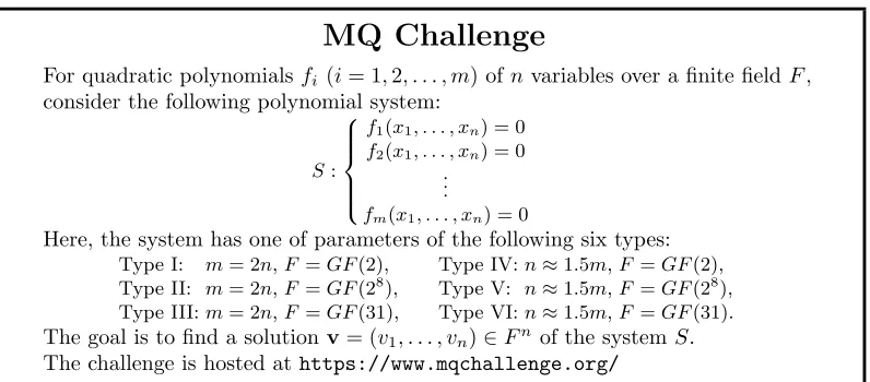
MQ Challenge
For quadratic polynomialsfi (i= 1,2, . . . , m) ofnvariables over a finite fieldF, consider the following polynomial system:
S:
f1(x1, . . . , xn) = 0
f2(x1, . . . , xn) = 0 .
..
fm(x1, . . . , xn) = 0
Here, the system has one of parameters of the following six types:
Type I: m= 2n,F =GF(2), Type IV:n≈1.5m,F =GF(2), Type II: m= 2n,F =GF(28), Type V: n≈1.5m,F =GF(28), Type III:m= 2n,F =GF(31), Type VI:n≈1.5m,F =GF(31).
Acknowledgments
We should like to thank Kouichiro Akiyama, Johannes Buchmann, Chen-Mou Cheng, Jintai Ding, Ryo Fujita, Keisuke Hakuta, Ludovic Perret, Albrecht Petzoldt, Shigeo Tsujii, and Bo-Yin Yang for their helpful comments and suggestions.
This work was supported by “Strategic Information and Communications R&D Promotion Programme (SCOPE), no. 0159-0091”, Ministry of Internal Affairs and Communications, Japan.
References
1. Bernstein D.J., Buchmann J. and Dahmen E., “Post Quantum Cryptography”, Springer, Heidelberg 2009.
2. Bettale L., Faug`ere J.C. and Perret L., “Hybrid Approach for Solving Multivariate Systems over Finite Fields”, Journal of Mathematical Cryptology, vol. 2, pp. 1–22, 2008.
3. Bardet M., Faug`ere J.-C., Salvy B. and Spaenlehauer P.-J. On the complexity of solving quadratic boolean systems.Journal of Complexity, vol. 29(1), pp. 53–75, 2013.
4. Berbain C. , Gilbert H., and Patarin J., “QUAD: A Practical Stream Cipher with Provable Security”, Eurocrypt 2006, Springer LNCS vol. 4004, pp. 109-128, 2006.
5. Bouillaguet C., Chen H-C., Cheng, C.-M., Chou T., Niederhagen R., Shamir A. and Yang B.-Y. Fast Exhaustive Search for Polynomial Systems inF2. CHES 2010, LNCS vol. 6225, pp. 203–218, 2010. 6. Buchberger B., “Ein Algorithmus zum Auffinden der Basiselemente des Restklassenringes nach einem
nulldimensionalen Polynomideal”, Ph.D. thesis, University of Innsbruch, 1965.
7. Buchberger B., Collins G.E., Loos R.G.K (Edts), in cooperation with Albrecht R. “Computer Algebra Symbolic and Algebraic Computation”, 296pages, (2nd edition) Springer-Verlag (Wien New-York), 1982-83.
8. Braeken A., Wolf C. and Preneel B., “A Study of the Security of Unbalanced Oil and Vinegar Signature Schemes”, CT-RSA 2005, Springer LNCS vol. 3375, pp. 29–43, 2005.
9. Chen A. I.-T., Chen M.-S., Chen T.-R., Cheng C.-M., Ding J., Kuo E. L.-H., Lee F. Y.-S., and Yang B.-Y., “SSE Implementation of Multivariate PKCs on Modern x86 CPUs”, CHES 2009, Springer LNCS vol. 5747, pp. 33–48, 2009.
10. Cheng C.-M., Chou T., Niederhagen R., and Yang B.-Y., “Solving Quadratic Equations with XL on Parallel Architectures”, CHES 2012, Springer LNCS vol. 7428, pp. 356–373, 2012.
11. Courtois N., Klimov A., Patarin J., Shamir A., “Efficient Algorithms for Solving Overdefined Systems of Multivariate Polynomial Equations”, Eurocrypt 2000, Springer LNCS, vol. 1807, pp. 392–407, 2000. 12. Courtois N. and Pieprzyk J. “Cryptanalysis of Block Ciphers with Overdefined Systems of
Equa-tions”, Asiacrypt 2002, Springer LNCS vol. 2501, pp. 267–287, 2002.
13. Courtois N., “The security of Hidden Field Equations (HFE)”, CT-RSA 2001, LNCS Springer vol. 2020, pp. 266–281, 2001.
14. Ding J., Gower J. E. and Schmidt D. S., “Multivariate Public Key Cryptosystems”, Advances in Information Security 25, Springer, 2006.
15. Ding J. and Schmidt D., “Rainbow, a New Multivariable Polynomial Signature Scheme”, ACNS 2005, Springer LNCS vol. 3531, pp. 164–175, 2005.
16. Ding J., Petzoldt A. and Wang L-C., “The Cubic Simple Matrix Encryption Scheme”, PQCrypto 2014, Springer LNCS vol. 8772, pp. 76–87, 2014.
17. Ding J., Wolf C., and Yang B.-Y., “ℓ-Invertible Cycles for Multivariate Quadratic (MQ) Public key Cryptography”, PKC 2007, Springer LNCS vol. 4450, pp. 266-281, 2007.
18. The Certicom ECC Challenge: https://www.certicom.com/index.php/ the-certicom-ecc-challenge
19. Faug`ere J.C., “A New Efficient Algorithm for Computing Groebner Bases (F4)”, Journal of Pure and Applied Algebra, vol. 139, pp. 61–88, 1999.
21. Faug`ere J.C., “On the Security of UOV”, In Proceedings of First International Conference on Sym-bolic Computation and Cryptography, SCC 2008, pp. 103–109, 2008.
22. Fouque P.-A., Macario-Rat G., Perret L., and Stern J., “Total Break of theℓ-IC Signature Scheme”, PKC 2008, Springer LNCS vol. 4939, pp. 1–17, 2008.
23. Kipnis A., Patarin J. and Goubin, L., “Unbalanced Oil and Vinegar Schemes”, Eurocrypt’99, Springer LNCS vol. 1592, pp. 206–222, 1999.
24. Kipnis A. and Shamir A., “Cryptanalysis of the HFE Public Key Cryptosystem by Relinearization”, CRYPTO’99, Springer LNCS vol. 1666, pp. 19–30, 1999.
25. The Lattice Challenge:http://www.latticechallenge.org/
26. Matsumoto T. and Imai H., “Public Quadratic Polynomial-tuples for Efficient Signature Verification and Message Encryption”, Eurocrypt’88, Springer LNCS vol. 330, pp. 419–453, 1988.
27. Patarin J., “Cryptanalysis of the Matsumoto and Imai public key scheme of Eurocrypt’88”, CRYPTO’95, Springer LNCS vol. 963, pp. 248–261, 1995.
28. Patarin J., “Hidden Field Equations (HFE) and Isomorphisms of Polynomials (IP): Two New Fam-ilies of Asymmetric Algorithms”, Eurocrypt’96, Springer LNCS vol. 1070, pp. 33–48, 1996.
29. Petzoldt A., Bulygin S., Buchmann J., “Selecting Parameters for the Rainbow Signature Scheme”, PQCrypto 2010, Springer LNCS vol. 6061, pp. 218–240, 2010.
30. Porras J., Baena J., and Ding J., “ZHFE, a New Multivariate Public Key Encryption Schem”, PQCrypto 2014, Springer LNCS vol. 8772, pp. 229–245, 2014.
31. The RSA Factoring Challenge: http://www.emc.com/emc-plus/rsa-labs/historical/ the-rsa-factoring-challenge.htm
32. Tao C., Diene A., Tang S., Ding J., “Simple Matrix Scheme for Encryption”, PQCrypto 2013, Springer LNCS vol. 7932, pp. 231–242, 2013.
33. Wolf C., “Introduction to Multivariate Quadratic Public Key Systems and their Applications”, In Proceedings of YACC 2006 - Yet Another Conference on Cryptography, Porquerolles, France, pp. 44–55, 2006.
34. Yang B.-Y. and Chen J.-M., “All in the XL Family, Theory and Practice”, ICISC 2004, Springer LNCS, vol. 3506, pp. 67–86, 2005.
35. Yasuda T., Takagi T., Sakurai K., “Security of Multivariate Signature Scheme Using Non-commutative Rings”, IEICE Transactions, vol. 97-A(1) pp. 245–252, 2014.
36. Homepage of the libFES library,http://www.lifl.fr/∼bouillag/fes/.
A
Input format of the MQ challenge
A.1 GF(2)
Galois Field : GF(2) Number of variables (n) : 4 Number of polynomials (m) : 8 Order : graded reverse lex order
The text box above is an example of a MQ challenge system over GF(2). As we can see in the example, are specified the coefficient field, the number of variables, the number of equations in the system, and the monomial order chosen for the MQ system. Every line ends up with the ; symbol. Data coming after the ************ line in he input file rerepesent polynomials. These data are made up of the coefficients of the polynomials in the monomial basis, with respect to the monomial order indicated. For the graded reverse lexicographic order, let x1, x2, x3 and x4 to be the four variables so thatx1> x2> x3> x4. The monomials are then ordered as follows: x2
1 > x1x2 > x1x3 > x1x4 > x22 > x2x3 > x2x4 > x23 > x3x4> x42 > x1 > x2 > x3 > x4 >1. Thus, the first polynomial isx1x3+x1x4+x2x3+x2x4+x23+x3x4+x24+x1+x2+ 1 and the second polynomial is x1x2+x1x3+x2x4+x23+x3+ 1.
A.2 GF(28)
Galois Field : GF(2)[x] / x∧8 + x∧4 + x∧3 + x∧2 + 1 Number of variables (n) : 4
Number of polynomials (m) : 8 Order : graded reverse lex order
*********************
de 8d 73 3b f0 46 88 50 ca 7b dc 9d 22 cd b2 ; e1 f7 ac 25 ed b9 74 9b 7b d4 94 4f e6 b5 e0 ; f2 cf c3 5d c4 cd a1 aa 20 51 85 4b dd b1 bc ; 08 4e 21 48 7e bc 7a ad de d5 0c b3 00 4f 5c ; 81 0e 98 4d 3c 38 d3 07 48 f3 5a 52 27 fc 91 ; ee 27 47 c9 82 21 99 31 0e cd c4 b8 69 69 9e ; 7b ce 96 c5 37 6a ce 34 ca 19 73 8f 30 34 b6 ; 90 65 bc d0 02 77 6c af 1d 7f 1c 29 9c 55 60 ;
A.3 GF(31)
Galois Field : GF(31) Number of variables (n) : 4 Number of polynomials (m) : 8 Order : graded reverse lex order
*********************
29 20 25 28 4 7 10 28 8 13 14 29 19 30 8 ; 24 20 3 27 25 28 30 3 23 6 23 25 3 2 18 ; 4 29 29 31 0 19 7 24 18 8 9 23 24 8 27 ; 28 4 4 4 17 16 3 25 14 2 1 6 30 8 16 ; 6 1 11 17 3 1 14 14 6 29 3 23 27 18 22 ; 25 19 7 0 1 14 28 27 6 11 13 26 29 14 24 ; 12 21 28 2 21 25 0 12 1 29 27 7 23 23 14 ; 1 28 21 15 11 30 23 7 9 26 10 29 2 0 7 ;