An iterative scheme for feature-based positioning using a
weighted dissimilarity measure
Caifa Zhou1,∗ ID, Andreas Wieser1
1
2
3
4
5
6
7
8
9
10
11
12
13
14
15
16
17
1 IGP,ETHZürich;{caifa.zhou,andreas.wieser}@geod.baug.ethz.ch * Correspondence:[email protected];Tel.:+41-44-633-3039
Abstract:Weproposeaniterativeschemeforfeature-basedpositioningusinganewweighteddissimilarity measurewiththegoalofreducingtheimpactoflargeerrorsamongthemeasuredormodeledfeatures. The weightsarecomputedfromthelocation-dependentstandarddeviationsofthefeaturesandstoredaspartof thereferencefingerprintmap(RFM). Spatialfilteringandkernelsmoothingofthekinematicallycollected rawdataallowefficientlyestimatingthestandarddeviationsduringRFMgeneration.Inthepositioningstage, theweightscontrolthecontributionofeachfeaturetothedissimilaritymeasure,whichinturnquantifiesthe differencebetweenthesetofonlinemeasuredfeaturesandthefingerprintsstoredintheRFM.Featureswith littlevariabilitycontributemoretotheestimatedpositionthanfeatureswithhighvariability. Iterationsare necessarybecausethevariabilitydependsonthelocation,andthelocationisinitiallyunknownwhenestimating theposition.UsingrealWiFisignalstrengthdatafromextendedtestmeasurementswithgroundtruthinan officebuilding,weshowthatthestandarddeviationsofthesefeaturesvaryconsiderablywithintheregionof interestandareneithersimplefunctionsofthesignalstrengthnorofthedistancesfromthecorresponding accesspoints.ThisisthemotivationtoincludetheempiricalstandarddeviationsintheRFM.Wethenanalyze thedeviationsoftheestimatedpositionswithandwithoutthelocation-dependentweighting.Inthepresent examplethemaximumradialpositioningerrorfromground trutharereduced by40% comparingtokNN withouttheweighteddissimilaritymeasure.
Keywords: weighted dissimilarity measure; feature-based indoor positioning; signals of opportunity; location-dependentstandarddeviation
18
1. Introduction 19
Feature-based (i.e. fingerprinting-based) indoor positioning systems (FIPSs), one of the promising indoor 20
positioning solutions, have been proposed using various types of features (e.g. WLAN/BLE signal strengths [1–3], 21
geomagnetic field strengths [4] or visible patterns [5]) for providing indoor location-based services (LBSs) to 22
pedestrians [6–8]. The positioning accuracy of the state-of-the-art FIPSs using the received signal strength (RSS) 23
of WLAN access points (APs) is in the range of a few meters [9]. This is adequate for pedestrian indoor 24
positioning and navigation in many cases. However, unexpected and unacceptably large errors (e.g.>20 m in 25
horizontal coordinates [10]) can be observed in real environments. They jeopardize the practical usability of 26
FIPSs [11,12]. Such large errors may be caused by large deviations of the measured or stored feature values 27
when performing the location estimation [13]. 28
In order to benefit from the attractive characteristics of FIPS while mitigating large errors, the trend is to 29
combine the feature-based positioning with other techniques. Such hybrid approaches combine the feature-based 30
information with e.g. pedestrian dead reckoning (PDR) [14], map matching [15,16] or infrared ranging [17]. In 31
addition, Bayes filtering methods, such as Kalman filters or particle filters are used to improve the estimated 32
trajectory of pedestrians by combining the measurements with assumptions on the user’s motion [14,18]. Merging 33
different positioning solutions may help mitigating the impact of large errors of individual observations on the 34
quality of a specific type of LBSs. However, such approaches requires either deploying additional infrastructure 35
or providing extra information (e.g. the indoor map). It would be useful to detect or mitigate large errors in FIPS 36
using only intrinsically available data. This has attracted little research attention in the past, see e.g. [11,12,19], 37
and is the motivation for the present contribution. 38
We base our approach on the variability of the feature values at each individual location. Feature values 39
measured during the positioning stage are snapshots affected by noise. Even if the expected value of the feature 40
has not changed since the data collection for the generation of the reference fingerprint map (RFM), the measured 41
value may be closer to the RFM value at a different position than to the one at the correct position because of 42
this noise. It is therefore important to take the noise into account when assessing the similarity of measured and 43
stored feature values. We facilitate this by storing the empirical standard deviations (STDs) in the RFM which 44
is generated during the offline phase for representing the relationship between locations and their associated 45
features. The estimation of the variability is carried out by empirically analyzing the spatial distribution of the raw 46
data (e.g. RSS values) included in the RFM. It yields an extended representation of the RFM, which contains not 47
only the spatially smoothed feature values, but also the location-wise estimated STD of each individual feature 48
(see Section4). These values can then be used to mitigate the impact of large errors in FIPS. To this end we 49
propose a weighted dissimilarity measure, which quantifies the difference between the online measured features 50
and the features stored in the RFM, by adapting the contribution of the individual features to the dissimilarity 51
measure relative to their estimated STD values (see Section5.1). The positioning process is carried out in an 52
iterative way because we need to assume the user’s location, which is required for retrieving the STD of the 53
online measured features (see Section5.2). Beyond the use further discussed in this paper, the location-dependent 54
standard deviations can also be employed for identifying (large) changes of features which may need an update 55
of the RFM, see e.g. [7,20,21]. 56
The remaining of the paper is organized as follows: Section2summarizes the work related to reducing 57
large errors in an FIPS. The fundamentals of the feature-based positioning are briefly described in Section3. The 58
robust estimation of the variability of the RFM and its application to positioning are presented in Section4and5, 59
respectively. Finally, the evaluation of the variability estimation as well as the positioning performance using the 60
iterative scheme are presented in Section6for a real world dataset. 61
2. Related work 62
Herein we focus on publications that address the detection and reduction of large errors in an FIPS. We 63
refer the interested readers to [6,7,9] for more general information about indoor positioning. A comprehensive 64
comparison of different feature-based indoor positioning algorithms using various similarity/dissimilarity metrics 65
is available in [22–24]. A short review of the methods used for generation or creation of the RFM can be found 66
in e.g. [7,25]. 67
[12] provides a detailed analysis of the sources of large errors when employing deterministic feature-based 68
positioning approaches (e.g. kNN). The analysis is based on simulations for different indoor scenarios. The 69
authors consider the influence of several factors such as the quantization error of signal acquisition, the density of 70
the reference measurements, and the selected dissimilarity metrics on the positioning error. The analysis shows 71
that large observation errors mostly occur at locations where both the mean and the maximum value of the RSS 72
are low. However, the authors do not report about a validation of their analysis in a really deployed FIPSs. On a 73
related note, [13] proposes to simply disregard features with a large standard deviation for the estimation of the 74
user’s position. 75
There are only few works that focus on reducing or estimating the positioning errors based on the analysis 76
of the RFM1. [11] introduces a weighted dissimilarity measure by computing the discriminative indicator for 77
each feature according to the Log-distance path loss model. However, the variability of the online measured 78
features which has an impact on the estimation of the discriminative factor is not taken into account. In [19] 79
and [26], the authors propose different regression models (e.g. neural networks, random forest, or Gaussian 80
processes) for estimating the positioning errors and uncertainties that can be used to improve the performance 81
1 [12] provides a complete discussion of the works focusing on reducing large positioning errors by support of other technologies (e.g.
of tracking a pedestrian’s trajectory. Even if this is not the focus of these papers, the results suggest that the 82
regression-based error prediction models cannot help to mitigatelargeerrors because the predicted errors have a 83
large uncertainty. 84
Compared to previous publications, we carry out the variability analysis of the RFM using a kinematically 85
collected dataset, which includes not only the noise originating from the short term fluctuations of the features 86
measured by a mobile device, but also the noise introduced by the motion status (e.g. moving speed and headings) 87
of the mobile device. This setup is closer to the realistic situation of positioning and tracking pedestrians. 88
The estimation of the variability is based solely on the raw RFM and is later used for reducing large errors by 89
introducing an iterative scheme with the weighted dissimilarity measure in the online positioning phase. 90
3. Feature-based positioning 91
We start this section by introducing the fundamental concepts of feature-based positioning and then briefly 92
describe the process of kinematically collecting the RFM. 93
3.1. Fundamental concepts 94
Each measured feature is uniquely identifiable and has a measured value. For example, the signal from an AP, 95
can be identified by its media access control address and is associated with an RSS. Features are thus formulated 96
as pairs of attributeaand valuev, i.e. (a,v). A measurement (i.e. fingerprint)Oui taken by the user u at the 97
location/timeiconsists of a set of measured features, i.e.Oui :={(auik,vuik)|au
ik∈A;vuik∈;k∈ {1, 2,· · ·,Niu}}, 98
whereAis the complete set of the identifiers of all available features andNiu(Niu=|Ou
i|) is the number of features
99
observed by the user u ati. The set of attributes ofOu
i is defined asAui :={auik|∃(auik,vik)∈Oui}(Aui ⊆A). 100
The positioning process consists of inferring the estimated user locationˆlui =f(Ou
i)(ˆlui ∈d)as a function of 101
the measurement and the RFMF, wheref is a suitable mapping algorithm from the measurement to location2. 102
F represents the relationship between the locationland the measurementO, i.e.F :l7→O|l∈Gthroughout 103
the region of interest (RoI)G. If the RFM is discretely represented, we denote it asF:={(lj,O˜j)|lj∈G,j∈ 104
{1, 2,· · ·,|F|}}(whereO˜ j=F(lj)). A discrete RFM can be obtained e.g. by collecting fingerprints at different
105
known or independently measured locations within the RoIG. 106
3.2. Kinematically acquired RFM 107
The kinematically obtained dataset used as the basis for the RFM herein has already been employed in [25]. 108
It was acquired using a mobile device (Nexus 6P) whose ground truth location was continuously measured with 109
mm- to cm-level accuracy by a total station tracking a mini prism mounted on top of the mobile device. This 110
procedure enables to simultaneously obtain accurate reference coordinates and the fingerprinting data collected 111
by a pedestrian. The measurements were obtained at arbitrary locations lying on the trajectory of a pedestrian 112
because the data acquisition on the mobile phone is passively triggered by the status of measurable features (e.g. 113
the arrival of new features or the change of feature values) [27]. By carrying out a thorough site-survey, all the 114
collected measurements and their tracked trajectories were merged and used to generate the raw RFM. Herein we 115
use this dataset as the basis of our analysis. More details of its acquisition and processing can be found in [25]. 116
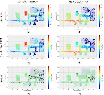
Fig.1aand1bshow examples of the raw data collected for RFM generation, namely the RSS values from 117
two WLAN APs. These are signals of opportunity as the APs had been installed for providing Internet access 118
and the signals are their anyway, when using them for the purpose of indoor positioning. The raw measurements 119
have been acquired at arbitrary locations throughout the RoI which consists of several rooms and corridors within 120
an office building. 121
AP:9c:50:ee:09:5f:30 AP:9c:50:ee:09:61:d1
Ra
w
RFM
(a) (b)
Spatially
filtered
RFM
(c) (d)
Residual
(e) (f)
Figure 1. Examples of the raw and spatially filtered RFM of two arbitrarily selected APs. Third row shows residuals between the spatially filtered RFM and the raw RFM. The density of the reference locations over the RoI varies due to different accessibility (e.g. areas blocked by furniture or other facilities) and by different visiting frequency of the users.
4. Robust estimation of the feature variability 122
To estimate the noise of the measurable features at each location throughout the RoI, the features would 123
have to be measured (ideally consecutively) multiple times at each location. However, even for a relatively sparse 124
set of reference points throughout the RoI this would be prohibitively time-consuming and labor-intensive. We 125
relax this requirement by assuming that the expected feature values change only little within a local, spatial 126
neighborhood. Therefore, instead of estimating the standard deviation from the data collected only at a single 127
location, we use all feature values obtained within a certain radius about a chosen reference location. The 128
corresponding data are identified within the time series of data resulting while the user walked through the RoI. 129
We denote these fingerprints askinematically collectedones. The estimation of the standard deviation is still 130
possible if a sufficient number of measurements is obtained in the proximity of each reference location (see Fig.1). 131
The measurements thus associated with an individual reference location contain data obtained consecutively 132
within a short time at slightly different positions, but also data collected a certain time interval apart (e.g. half an 133
hour) because the user passed most locations several times during the entire data collection process. The resulting 134
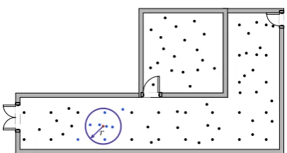
Figure 2.Schematic representation of the spatial filtering
measurement, which will also apply during the positioning stage. We thus consider the kinematically collected 136
RFM data suitable for the variability analysis. 137
Under the assumption that the expected value of each feature is locally obtainable, the location-wise STD of 138
each feature can be approximated based on the measurements associated to the neighborhood of a given reference 139
location. More formally, we estimate the STDσjkofk-th (k={1, 2,· · ·,|O˜ j|}) feature at the reference location 140
ljin the RFMF. These estimated values of the STD are later included in the extended representation of the RFM, 141
i.e.F:={lj,S˜j}withS˜j={(ajk,vjk,σjk)|ajk∈A˜ j}. We start the estimation of the feature values for the RFM
142
by applying a spatial median filter to the raw measurements in order to mitigate potential outliers. We proceed 143
with the kernel smoothing (KS) that enables us to reduce the impact of noise and obtain a quasi-continuous 144
representation of the RFM by interpolation. It allows us to approximate the expected value of the measurements 145
at any location throughout the RoI. We perform spatial filtering and KS in two separate steps because KS is 146
non-robust and the preceding filtering allows us to remove outliers before filtering noise and interpolating. The 147
location-wise STD for each measurable feature is finally calculated as empirical standard deviation of the raw 148
measurements (before filtering and kernel smoothing) within a neighborhood of the specific reference points. In 149
the following, the individual steps of the algorithm are explained in more detail. 150
As can be seen in Fig.1aand1bthe measured feature values in the neighborhood of a given location may 151
vary significantly. This is particularly visible around locations with very low signal strength values, i.e. values 152
close to the sensitivity limit of the mobile devices. In order to mitigate the impact of these variations on the 153
representation of the RFM, we apply the spatial filtering which replaces the originally measured feature valueva 154
of featureaat the given locationlby the median value of the values measured within the neighborhood ofl. We 155
have chosen to defined the neighborhood as the set of measurements collected at the up tomlocations closest tol 156
that at the same time lie within the given radiusraboutl(see the schematic in Fig.2). 157
In the second step, we estimate a continuous RFM using KS in order to be able to retrieve the expected 158
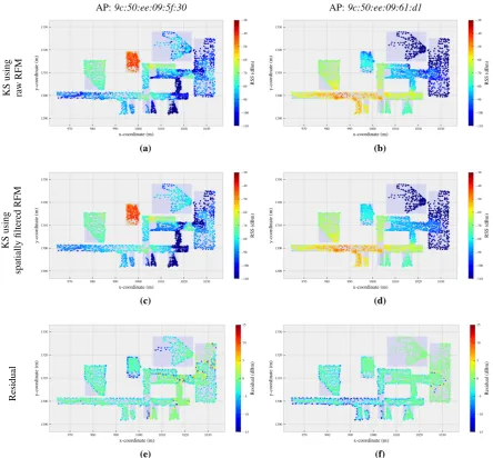
measurements at any location within the RoI [28]. Albeit KS can reduce noise by implicit filtering, it is not 159
robust and the results could therefore be severely contaminated by outliers in the measured features (Fig.3aand 160
3b). Therefore, we apply KS to the media filtered data rather than to the original ones. Because the structure 161
of the indoor region is not taken into account, KS tends to smoothen the RFM over discontinuities like large 162
changes of feature values or change from feature presence to feature absence over short distances e.g. because of 163
walls. This over-smoothing degrades the quality of the RFM for certain features at certain locations. This may be 164
relevant for positioning [29], especially when using radio frequency signals such as WLAN whose propagation 165
is highly influenced by obstacles. Herein we employ a modified version of KS which uses only a subset of the 166
data in the neighborhood of a given location for approximating the expected feature values [28]. This alleviates 167
the impact of over-smoothing, while at the same time reducing the computational complexity [28,30].3. 168
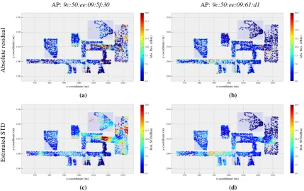
The distribution of the measured noise shown in Fig.4 clearly suggests that the variances are 169
location-dependent, are different for different features, and cannot be represented as just a function of feature 170
value or of geometric distance from a single point per feature (e.g. the AP location). So, we propose to model the 171
3 A detailed analysis of the over-smoothing problem, the computational complexity of KS, and a discontinuity preserving approach to KS
STD as a location-dependent quantity, independently for each individual feature. To this end, we compute the 172
absolute residuals of the raw data with respect to the spatially filtered and kernel smoothed RFM in order a robust 173
estimate of the STD. At the reference locationljin the RFMF, the STDσjkofk-th (k={1, 2,· · ·,|O˜ j|}) feature 174
contained inO˜ jis computed by the median absolute deviation (MAD) of the measured feature values associated 175
to locations defined as the support set for spatial filtering. The extended representation of the RFM with the 176
estimated STD at locationljis denoted asS˜j={(ajk,vjk,σjk)|ajk∈A˜ j}and is continuously represented using 177
KS, i.e.S˜j:=F(lj). 178
5. Iterative scheme for online positioning 179
Inspired by the finding that the variability of the features has a large effect on the positioning error [13], 180
we employ the robustly estimated STD of the features to reduce the impact of uncertain feature values when 181
calculating the position estimate. We construct a weighting scheme that reduces the weight of a feature with high 182
STD relative to features with low STD. Therefore, a discrepancy between online measured and expected value of 183
a feature with low STD has more impact on the dissimilarity measure—and thus on the estimated position—than 184
the same discrepancy for a feature with a high STD. This dissimilarity measure is used to identify which subset 185
of reference locations is taken into account when inferring the user’s location using deterministic feature-based 186
positioning algorithms such askNN. 187
5.1. Weighted dissimilarity measure 188
Given the online measured featuresOui at the locationlui, the weighted dissimilarity measuredwbetween
Ou
i and the j-th reference fingerprintO˜jstored in the RFM is computed as:
dw(Oui,O˜ j) =
∑
a∈Aui∩A˜j
wuikg(vuik,vjk) +α1·
∑
a∈Au i\A˜j
wuikg(vuik,γ) +α2·
∑
a∈A˜j\Au i
wuikg(γ,vjk) (1)
whereg is the selected dissimilarity measure (e.g. Minkowski distance) andγ is the missing value indicator
189
(e.g. -110 dBm). This equation represents a compound dissimilarity measure (CDM) as defined in [31], and 190
correspondinglyα1andα2are hyperparameters regulating the contribution of mutually unshared features to 191
the dissimilarity measure. However, the CDM herein uses a new distance metric, not covered in [31], by 192
location-wise weighting of individual features instead of only weighting according to the respective observability. 193
wuikis the weight of thek-th feature at the location/timeiand is computed by employing the variability derived 194
from the estimated expected measurementS˜ui obtained atlui. In case that thek-th feature inA˜i j(A˜i j:=Au
i∪A˜j) 195
is not measurable at locationlui, the weight of the corresponding feature is set to the minimum value of the 196
weights of the measurable features thus reducing their impact on the estimation of the location. 197
We selected the softmax function [32,33]
wuik= e
−β σik−2
|S˜u i|
∑ l=1
e−β σlk−2
(2)
to calculate the weight of each feature using the estimated STD, whereS˜ui =F(lui)andβ>0 is the scale factor 198
for adapting the concentration of the softmax function. The denominator normalizes the weights and makes the 199
solution invariant to the scale of the weights. We have also tried to use a weight function corresponding to the 200
one frequently employed for weighted least-squares (and actually motivated by maximum likelihood estimation 201
with normally distributed observations), namely setting each weight proportional to the inverse of the respective 202
variance. However, the accuracy of the solutions was worse than using the softmax function. 203
The weighted dissimilarity measure is used to identify the candidate locations, whose dissimilarity values 204
are smallest among all reference fingerprints stored in the RFM. We estimate the user’s location usingkNN 205
or weightedkNN by averaging or weighted averaging (e.g. inversely proportional to the value of dissimilarity 206
5.2. Iterative scheme 208
The position estimation requires to calculate the weight of each feature. However, the weight depends on 209
the standard deviation which in turn varies with location. The required value can only be extracted from the 210
RFM once the location is known. We thus carry out the positioning in an iterative way by i) assuming a position 211
(initialization); ii) retrieving the STDs from the RFM, calculating the weights and estimating the position (update 212
step); and iii) repeating ii) until a termination condition of the iterative scheme is fulfilled. These steps are 213
explained in more detail in the following subsections. 214
5.2.1. Determination of the initial location 215
The initial locationˆl(0)i of the user is used to derive the weights for the first iteration. One straightforward 216
way of initializing is to choose the location estimated by the standardkNN without the weighted dissimilarity 217
measure (i.e. the traditionalkNN). When processing real world data we found out that the solution obtained at 218
the termination of the iterative process is quite stable when initializing the location even randomly (see Section 219
6). This suggests that the positioning performance does not depend strongly on the choice of the initial location. 220
5.2.2. Update step 221
At thet-th iteration (t∈+), the weights as well as the dissimilarities are computed according to the variability obtained at the location searched at the(t−1)-th iteration. The weightw(t)ik of thek-th feature at location/timeiand thet-th iteration is defined as:
w(t)ik = e
−β σlk(t−1) −2
|S˜(it−1)| ∑ l=1
e−β σ (t−1) lk
−2
(3)
whereS˜(ti−1)is the estimated expected value of features with their STD at locationˆl(t−1). This updated weights 222
are used to compute the dissimilarity measure as defined in (1) and consequently to infer the estimated location 223
ˆl(t)i at thet-th iteration using e.g.kNN algorithm. 224
5.2.3. Termination condition 225
Ideally the searching process should converge to a fixed location. This state is assumed to be reached when the distance between two consecutively obtained location estimated is lower than a given small threshold. We denote this subsequently as converging state and terminate the iterative process when
|ˆl(t)i −ˆl(ti−1)|2<dmin,
wheredminis the threshold, which we set to 10−3m in the experimental analysis later on. We found out that the iterative process proposed herein sometimes enters a loop in which a (small) subset of locations are repeatedly obtained as estimates in the same sequence. We denote this as the looping state and introduce a second termination condition which is met when this state is recognized. We implement it as a threshold on the distance between the location estimate obtained at the iterationtand the ones estimated at previous iterations except the estimated location at the(t−1)-th iteration. More formally, the second condition is satisfied and the iteration is terminated when
min m=1,···,t−2{|ˆl
(t)
i −ˆl
(m)
i |2}<dmin.
Finally, the maximum numberT of iterations is also limited (e.g. T =100) in order to prevent long or 226
endless search for a solution. If the search for an estimate is terminated due to this condition, we denote it as 227
max. state. 228
Assuming that the iterations terminate afterT0iterations we select or compute the final estimate of the 229
position depending on the termination flag (TF)εiu∈ {0, 1, 2}, indicating the respective state, as follows:
• Converging state: The location estimated at theT0-th iteration is selected as the final estimate of the 231
user’s locationˆlui, andεiuis set to 0.
232
• Looping state: In this case the searched locations do not converge to a single point. If the number of 233
locations exceeds a certain minimum (e.g. 4) and if the locations visited in the looping state are not farther 234
apart than a chosen maximum (e.g. 0.01 m) (see Fig.5) we use the minimum covariance determinant (MCD) 235
estimator4for computing the estimated locationˆlu
i of the user from the convex hull of the visited locations. 236
If the number of points is too low or if they are too far apart from each other the situation is handled like the 237
max. state. If the looping state termination condition is met and the MCD is reported as the final estimate, 238
the TFεiuis set to 1.
239
• Max. state: This case actually means that the position estimation using the weighted dissimilarity measure fails because no position can be found where the measured features and the predetermined standard deviations are compatible. In this case, we can either report a failure of the algorithm and not calculate a solution, or we can calculate an estimate ignoring the variability information. We have chosen the latter herein. In particular, we determineˆlui from all searched locations Lˆ analyzing the similarities between the user measured fingerprintOu
i and the expected ones at the searched locations. Specifically, we employ the modified Jaccard index (MJI), which has been used for identifying subregions according to the measurability of features [25], as the similarity metric. The MJI valueSMJIbetweenOu
i and the expected oneO˜ˆ(t)i (O˜ˆ(t)i :=F(ˆli(t)))at the searched locationˆl(t)i of thet-th iteration is computed by:
SMJI(Oui,O˜ˆ(t)i ) =1 2
|Au i∩A˜ˆ
(t)
i |
|Au
i∪A˜ˆ
(t)
i | +|A
u
i∩A˜ˆ
(t)
i | |Au
i|
(4)
whereAui andA˜ˆ(t)i are the sets of the measured features contained inOui andO˜ˆ(t)i , respectively. The 240
estimated user’s locationˆlui is then the one that has the biggest MJI value among all searched locationsLˆ, 241
i.e. the one with the maximum number of common measurable features is selected as the final estimate of 242
the user’s location. 243
6. Analysis of the variability estimation and positioning performance 244
We start this section by presenting the results of the location-wise variability of each individual feature 245
estimated using the kinematically collected RFM data, which is discussed in detail in [25]. We conclude this 246
section with an analysis concerning the characteristics of iteratively searched locations as well as the positioning 247
performance of the proposed iterative scheme. 248
6.1. Results of the variability estimation 249
Herein we setm=20 andr=2 m to obtain the spatially filtered RFM, which visually has an adequate 250
spatial consistency in the neighborhood of each location. Fig.1cand1dclearly show that the spatial filtering 251
can reduce the large variations contained in the raw RFM to a great extent. For further analysis, we compute 252
the residuals between the raw and the spatially filtered RFM. The obtained residuals are close to zero-mean 253
distributed and have a location-dependent magnitude as illustrated in Fig.1eand1f. Large residuals occur either 254
in regions close to the boundaries of the RoI (e.g. close to the walls or corners of rooms and corridors) or at 255
locations where the RSS values are hardly measurable by the mobile phone. In both cases the features are very 256
likely affected by obstacles which also cause locally large variations of the feature values. 257
Fig.4shows the results of the estimated STD value using the MAD of the measured feature values associated 258
to the neighborhood of a given location. As can be seen, each feature has a different variability throughout 259
the RoI, i.e. the STD value is dependent both on the feature as well as on the location. This is the primary 260
motivation that the variability is modeled location-wise for each individual feature instead of simply expressing 261
AP:9c:50:ee:09:5f:30 AP:9c:50:ee:09:61:d1
KS
using
ra
w
RFM
(a) (b)
KS
using
spatially
filtered
RFM
(c) (d)
Residual
(e) (f)
Figure 3.Examples of kernel smoothed RFM of two arbitrary selected APs. The results of the first two rows are yielded by taking the raw RFM and the spatially filtered one (i.e. the ones depicted in the first two rows of Fig.1) as the input to KS, respectively. Third row shows the residual between the kernel smoothed RFM using the spatially filtered one and the spatially filtered RFM. Though the KS provides the continuous representation of the RFM, we only visualize the smoothed features at the locations contained in the raw RFM for easy comparison.
the variability as a function of the measured feature value or as a constant value. The regions where the feature 262
values have a higher STD are clearly correlated to the local variations of the measured feature value and the 263
geometry of the building (Fig.3and4). The high variances occur in the case that a low number of measurements 264
has been collected in the neighborhood region. These are caused by the violation of the assumption that the 265
expected feature values are locally obtainable. 266
6.2. Results of iterative scheme for positioning 267
The proposed iterative scheme for feature-based positioning is implemented using the application 268
programming interface of scikit-learn package, a widely used machine learning package in Python [34]. Herein 269
we present the results of the iterative positioning using kNN with the weighted Euclidean distance as the 270
dissimilarity metric for measuring the distance in the feature space. The values of several hyperparameters have 271
to be configured. Regarding the weighted dissimilarity measure, as formulated in Section5.1,α1andα2are 272
AP:9c:50:ee:09:5f:30 AP:9c:50:ee:09:61:d1
Absolute
residual
(a) (b)
Estimated
STD
(c) (d)
Figure 4.Examples of the absolute residuals and estimated STD for two APs
and the scale factorβ of the softmax function are empirically set to 1 and 2.0, respectively. Optimization of the 274
parameters (e.g. using grid/random search or Bayesian optimization [35]) for achieving the best positioning 275
performance is left for future work. 276
Fig.5shows several examples of the searched locations of the iterative positioning with random as well as 277
kNN initialization. Each individual subplot depicts the results of the iterative positioning at a fixed test location. 278
The subplots depict the searched locations (red squares), the final estimation (blue triangle or coral diamond), 279
the estimation using the traditionalkNN algorithm, and the ground truth (black square)5. The initialization of
280
the initial location has only a minor impact on the iterative searching process in this case because the RoI is 281
relatively small. The initial location is determined by arbitrarily taking one of the reference locations stored in 282
the RFM in case of random initialization. In addition, our schemes for determining the final estimation of the 283
user’s location from these searched locations do not achieve the best potential positioning performance using the 284
iterative scheme. Because there are locations inLˆ that are closer to the ground truth but they are not taken as the 285
final estimation. This suggests that the iterative scheme for positioning has the potential to further improve the 286
positioning performance if the proper technique is applied to retrieve the final estimation from these searched 287
locations. The optimal positioning accuracy (denoted as Ours (opt.) in Fig.8and in TABLE1) is defined by 288
assuming that the technique for the final estimation is capable of retrieving the searched location that is the closest 289
to the ground truth. As depicted in Fig.8, our scheme for retrieving the final estimation can achieve comparable 290
performance to that of the optimal one when comparing the overall positioning accuracy. However, from TABLE 291
1, it also suggests that the maximum positioning error can be reduced to a large extent if the optimal positioning 292
can be achieved. 293
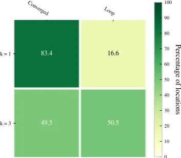
Fig.6shows the statistics of the TF, denoted by the percentage of locations terminated with different 294
conditions. In case ofk=1 about 83% iterative search processes have terminated with the converging state. This 295
is about 35 percent points higher than in case ofk=3. We therefore set the number of the nearest neighbors for 296
kNN to 1. In addition, we have analyzed the searched locations within the looping state cases are distributed on 297
kNN initialization Random initialization 1 Random initialization 2
Loc.
1
(a) (b) (c)
Loc.
2
(d) (e) (f)
Loc.
3
(g) (h) (i)
Ours (conv.)
Ours (loop.)
Figure 5.Examples of iteratively searched location with different initializations. The locations with black circles are repeatedly searched in the same sequence (i.e. the looping state) when using the iterative scheme.
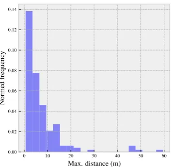
space. Fig.7shows the distribution of the maximum distance between points within the same loop. Most of the 298
maximum distances are significantly less than 10 m, though, in some extreme cases we observed up to 60 meters. 299
As shown in Fig.8, the schemes proposed for the loop state (MCD or MJI) are still capable of properly selecting 300
position estimates close to the ground truth also in most of these cases.
Figure 6.Comparison of the percentage of locations terminated with different conditions fork=1 and 3. The max. state is not included in the figure because it has not happened in the experimental analysis.
301
The empirical cumulative distribution function (ECDF) of the radial positioning errors is presented in Fig.8. 302
Figure 7.The maximum distance between the locations consisting of the loop state fork=1
of the traditionalkNN andkNN with CDM. Using the algorithm proposed herein, about 86% of the estimated 304
locations have a positioning error smaller than 2 m and around 97% of estimated locations have an error of less 305
than 4 m. Compared tokNN, this represent an improvement of up to 20 and 10 percent points, respectively. The 306
improvement is also up to 10 and 6 percent points as compared tokNN with CDM. The percentage of estimated 307
locations whose error distance is larger than 5 m is reduced from about 10.2% and 6.7% to 2.6%, when compared 308
to the traditionalkNN, andkNN with CDM, respectively. We also report the circular error (CE) defined as the 309
minimum radius for including a given percentage of positioning errors (e.g. CE 50 for the 50thpercentile) in
310
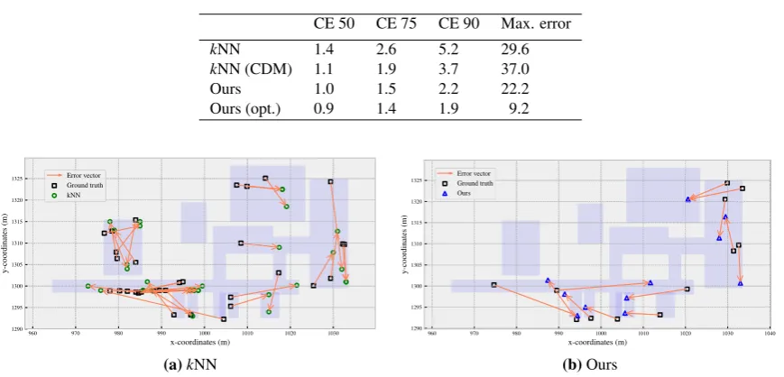
TABLE1. The maximum positioning error is reduced by about 40%, from 37.0 m to 22.2 m when comparing 311
kNN with CDM to our approach. The CE 50, CE 75, and CE 90 are reduced by one third when compared to 312
thekNN without iterative positioning. Furthermore, in Fig.9we illustrate and compare the distribution of the 313
locations, at which the positioning error is larger than 8 m using the originalkNN. Fig.9ashows that these 314
locations yielding large errors are mostly located close to the accessible boundaries of the indoor regions, i.e. 315
close to corners of corridors and rooms, or to the walls. This pattern is similar to the spatial distribution of high 316
variance of the feature values contained in the raw RFM as shown in Fig.4. Our approach can significantly reduce 317
the number of occurrences where the positioning errors are larger than 8 m. 318
Figure 8.Comparison of ECDF with respect to the radial positioning errors.
7. Conclusion 319
We have proposed an iterative scheme for feature-based positioning, which is based on the weighted 320
dissimilarity measure, for reducing large errors occurring in FIPSs. Appropriate weights for the individual feature 321
Table 1.Statistics of positioning errors (meters) CE 50 CE 75 CE 90 Max. error
kNN 1.4 2.6 5.2 29.6
kNN (CDM) 1.1 1.9 3.7 37.0
Ours 1.0 1.5 2.2 22.2
Ours (opt.) 0.9 1.4 1.9 9.2
(a)kNN (b)Ours
Figure 9.Distribution of the locations yielding large errors (>8 m) in positioning
location-wise standard deviation of each feature is robustly computed using the MAD between the raw data and 323
the spatially smoothed RFM. This variability information is stored as an additional layer of the RFM and used 324
for weighting the contribution of each feature to the dissimilarity measure during the online positioning phase. 325
Using real WLAN RSS data collected along with location ground truth in an office building, we could show 326
that the noise of the raw observations indeed depends on the location and on the feature. We have implemented the 327
proposed algorithms in Python and have validated the performance of the proposed iterative scheme. Compared 328
tokNN with CDM, the maximum positioning error is reduced by more than 40% and the iterative scheme can 329
improve the overall positioning performance. The positioning accuracy defined as the percentage of the locations 330
whose radial positioning error is less than 2 m is improved from 65% to 86% when compared to traditionalkNN. 331
In future work, we will further investigate the proposed algorithms using data from other environments. We 332
will further investigate the loop state and the handling of remaining outliers. Finally, we will investigate how the 333
standard deviations modeled within the RFM can help to identify the need for updates of the RFM. 334
Acknowledgment 335
The Chinese Scholarship Council has supported C. Zhou during his doctoral studies at ETH Zürich. The 336
data used within the experimental investigation were collected by the students E. Weiss, I. Bai, N. Meyer, and 337
References 339
1. Padmanabhan, P.B.; N., V.; N., V. RADAR: An in-building RF based user location and tracking system. 340
Proceedings IEEE INFOCOM 2000. Conference on Computer Communications. Nineteenth Annual Joint Conference
341
of the IEEE Computer and Communications Societies (Cat. No.00CH37064)2000, 2, 775–784, [1106.0222]. 342
doi:10.1109/INFCOM.2000.832252. 343
2. Youssef, M.; Agrawala, A. The Horus location determination system. Wireless Networks2008,14, 357–374. 344
doi:10.1007/s11276-006-0725-7. 345
3. Zhuang, Y.; Yang, J.; Li, Y.; Qi, L.; El-Sheimy, N. Smartphone-based indoor localization with bluetooth low energy 346
beacons.Sensors2016,16, 596. 347
4. He, S.; Shin, K.G. Geomagnetism for smartphone-based indoor localization: Challenges, advances, and comparisons. 348
ACM Computing Surveys (CSUR)2018,50, 97. 349
5. Guan, K.; Ma, L.; Tan, X.; Guo, S. Vision-based indoor localization approach based on SURF and landmark. 2016 350
International Wireless Communications and Mobile Computing Conference (IWCMC). IEEE, 2016, pp. 655–659. 351
6. Brena, R.F.; García-Vázquez, J.P.; Galván-Tejada, C.E.; Muñoz-Rodriguez, D.; Vargas-Rosales, C.; Fangmeyer, J. 352
Evolution of indoor positioning technologies: A survey. Journal of Sensors2017,2017. 353
7. He, S.; Chan, S.H.G. Wi-Fi fingerprint-based indoor positioning: Recent advances and comparisons. IEEE
354
Communications Surveys & Tutorials2016,18, 466–490. 355
8. Pei, L.; Zhang, M.; Zou, D.; Chen, R.; Chen, Y. A survey of crowd sensing opportunistic signals for indoor 356
localization. Mobile Information Systems2016,2016. 357
9. Mautz, R. Indoor positioning technologies. Habilitation Thesis, Department of Civil, Environmental and Geomatic
358
Engineering, ETH Zurich, Switzerland2012. 359
10. Torres-Sospedra, J.; Jiménez, A.; Knauth, S.; Moreira, A.; Beer, Y.; Fetzer, T.; Ta, V.C.; Montoliu, R.; Seco, F.; 360
Mendoza-Silva, G.; others. The smartphone-based offline indoor location competition at IPIN 2016: Analysis and 361
future work. Sensors2017,17, 557. 362
11. Wu, C.; Yang, Z.; Zhou, Z.; Liu, Y.; Liu, M. Mitigating large errors in WiFi-based indoor localization for smartphones. 363
IEEE Transactions on Vehicular Technology2017,66, 6246–6257. 364
12. Torres-Sospedra, J.; Moreira, A. Analysis of sources of large positioning errors in deterministic fingerprinting. 365
Sensors2017,17, 2736. 366
13. Kaemarungsi, K.; Krishnamurthy, P. Analysis of WLAN’s received signal strength indication for indoor location 367
fingerprinting.Pervasive and Mobile Computing2012,8, 292 – 316. Special Issue: Wide-Scale Vehicular Sensor 368
Networks and Mobile Sensing, doi:https://doi.org/10.1016/j.pmcj.2011.09.003. 369
14. Li, X.; Wang, J.; Liu, C.; Zhang, L.; Li, Z. Integrated WiFi/PDR/smartphone using an adaptive system noise extended 370
Kalman filter algorithm for indoor localization. ISPRS International Journal of Geo-Information2016,5, 8. 371
15. Wang, J.; Hu, A.; Liu, C.; Li, X. A floor-map-aided WiFi/pseudo-odometry integration algorithm for an indoor 372
positioning system.Sensors2015,15, 7096–7124. 373
16. Wang, H.; Sen, S.; Elgohary, A.; Farid, M.; Youssef, M.; Choudhury, R.R. No need to war-drive: Unsupervised 374
indoor localization. Proceedings of the 10th international conference on Mobile systems, applications, and services. 375
ACM, 2012, pp. 197–210. 376
17. Bitew, M.A.; Hsiao, R.S.; Lin, H.P.; Lin, D.B. Hybrid indoor human localization system for addressing the issue of 377
RSS variation in fingerprinting. International Journal of Distributed Sensor Networks2015,11, 831423. 378
18. Röbesaat, J.; Zhang, P.; Abdelaal, M.; Theel, O. An improved BLE indoor localization with Kalman-based fusion: 379
An experimental study.Sensors2017,17, 951. 380
19. Lemic, F.; Handziski, V.; Aernouts, M.; Janssen, T.; Berkvens, R.; Wolisz, A.; Famaey, J. Regression-Based 381
Estimation of Individual Errors in Fingerprinting Localization. IEEE Access2019,7, 33652–33664. 382
20. Tao, Y.; Zhao, L. A Novel System for WiFi Radio Map Automatic Adaptation and Indoor Positioning. IEEE
383
Transactions on Vehicular Technology2018,67, 10683–10692. doi:10.1109/TVT.2018.2867065. 384
21. He, S.; Ji, B.; Chan, S.H.G. Chameleon: Survey-Free Updating of a Fingerprint Database for Indoor Localization. 385
IEEE Pervasive Computing2016,15, 66–75. doi:10.1109/MPRV.2016.69. 386
22. Retscher, G.; Joksch, J. Comparison of Different Vector Distance Measure Calculation Variants for Indoor Location 387
Fingerprinting. Location-Based Services (LBSs), 2016 International Conference on. ICA Commission on LBSs, 388
23. Torres-Sospedra, J.; Montoliu, R.; Trilles, S.; Belmonte, A.; Huerta, J. Comprehensive analysis of distance and 390
similarity measures for Wi-Fi fingerprinting indoor positioning systems. Expert Systems with Applications2015, 391
42, 9263 – 9278. doi:https://doi.org/10.1016/j.eswa.2015.08.013. 392
24. Minaev, G.; Visa, A.; Piché, R. Comprehensive survey of similarity measures for ranked based location fingerprinting 393
algorithm. 2017 International Conference on Indoor Positioning and Indoor Navigation (IPIN), 2017, pp. 1–4. 394
doi:10.1109/IPIN.2017.8115922. 395
25. Zhou, C.; Wieser, A. Modified Jaccard index analysis and adaptive feature selection for location 396
fingerprinting with limited computational complexity. Journal of Location Based Services2019, 13, 128–157, 397
[https://doi.org/10.1080/17489725.2019.1577505]. doi:10.1080/17489725.2019.1577505. 398
26. Li, Y.; Gao, Z.; He, Z.; Zhuang, Y.; Radi, A.; Chen, R.; El-Sheimy, N. Wireless fingerprinting uncertainty prediction 399
based on machine learning. Sensors2019,19, 324. 400
27. Schulz, M.; Link, J.; Gringoli, F.; Hollick, M. Shadow Wi-Fi: Teaching Smartphones to Transmit Raw Signals and 401
to Extract Channel State Information to Implement Practical Covert Channels over Wi-Fi. Proceedings of the 16th 402
Annual International Conference on Mobile Systems, Applications, and Services; ACM: New York, NY, USA, 2018; 403
MobiSys ’18, pp. 256–268. doi:10.1145/3210240.3210333. 404
28. Berlinet, A.; Thomas-Agnan, C.Reproducing Kernel Hilbert Spaces in Probability and Statistics; Springer Science & 405
Business Media: Berlin Heidelberg, 2011. 406
29. Bong, W.; Kim, Y.C. Fingerprint Wi-Fi Radio Map Interpolated by Discontinuity Preserving Smoothing. Convergence 407
and Hybrid Information Technology; Springer Berlin Heidelberg: Berlin, Heidelberg, 2012; pp. 138–145. 408
30. Cormen, T.H.; Leiserson, C.E.; Rivest, R.L.; Stein, C.Introduction to Algorithms, Third Edition, 3rd ed.; The MIT 409
Press, 2009. 410
31. Zhou, C.; Wieser, A. CDM: Compound Dissimilarity Measure and an Application to Fingerprinting-Based 411
Positioning. 2018 International Conference on Indoor Positioning and Indoor Navigation (IPIN), 2018, pp. 1–7. 412
doi:10.1109/IPIN.2018.8533681. 413
32. Murphy, K.P.Machine Learning: A Probabilistic Perspective; The MIT Press, 2012. 414
33. Gal, Y.; Ghahramani, Z. Dropout as a bayesian approximation: Representing model uncertainty in deep learning. 415
international conference on machine learning, 2016, pp. 1050–1059. 416
34. Pedregosa, F.; Varoquaux, G.; Gramfort, A.; Michel, V.; Thirion, B.; Grisel, O.; Blondel, M.; Prettenhofer, P.; Weiss, 417
R.; Dubourg, V.; Vanderplas, J.; Passos, A.; Cournapeau, D.; Brucher, M.; Perrot, M.; Duchesnay, E. Scikit-learn: 418
Machine Learning in Python.Journal of Machine Learning Research2011,12, 2825–2830. 419
35. Wang, Z.; de Freitas, N. Theoretical Analysis of Bayesian Optimisation with Unknown Gaussian Process 420