Evaluation of Epidemic Routing Protocol in Delay
Tolerant Networks
D. Kiranmayi
Department of CSE,
Vignan’s Institute Of IT, Visakhapatnam, India
ABSTRACT:There are many routing protocols that which can the handle the packet transmission in Delay Tolerant Networks and Ad-hoc networks. The communication may break or communication link may not exist at some instance. The Epidemic routing protocols have much number of applications in these DTNs. The Epidemic is an efficient protocol but it has some drawbacks like it consumes more Buffer size, bandwidth and Channel. So, the Enhanced Epidemic will deal with the above three problems with the techniques like sending Anti-packets (like acknowledgements), setting EC + TTL and setting TTL.
Index Terms: Delay tolerant networks, Epidemic routing protocol, Anti packets, EC+TTL
1 INTRODUCTION
The Routing can be a Static Routing or Dynamic Routing. The dynamic routing describes the capability of a system, through which routes are characterized by their destination. We have a network called Delay Tolerant Network (DTNs)
which represents a unique wireless network where the mobile nodes may not have a continuous communication with each other. The DTN do not have any topological information, uncertain between nodes. The communication link is unstable, frequent delays and frequent disruptions. For this we use mobile relay nodes for carrying and forwarding the messages and make communication possible among these nodes.The protocols like Epidemic, Data ferry and Statistical routing protocols were proposed to work in DTNs [2]. In this paper we are going to discuss about the Epidemic protocol. The Epidemic protocol will make packet delivery with fewer delays with more resources.
2 EPIDEMIC PROTOCOLS
Epidemic routing algorithm which was initially introduces by Demers for Data base Maintenance which uses the Replication method. Then Vahdat modified it as a flooding based algorithm which works in DTNs [3].
The Epidemic routing protocol floods the messages into the network (Neighbor nodes).The source node sends copy of message each and every node that it meets as shown in fig1. The nodes that receive copy of message will again sent to other nodes. Finally the destination will get the message [1].
Fig:1 Working of Epidemic
The Epidemic routing protocol explores all available communication paths [3] to deliver the messages and makes redundancy at each node.
This is protocol is simple, but it uses more storage, more bandwidth and nodes power due to sending the same message many times. It drops the messages at receiver when the resources reach the peak level [3]. It is especially useful when the Topology information is not known. To control the above issues, we implement the following …
Epidemic with Anti- Packets: These packets act as acknowledgements. By these Anti packets we can discard some of the packets from the Source node (which were received by the destination)[2]. These anti-packets may tell the source about what packets the destination received or what packets that it wants to receive.
Epidemic with Encounter Count (EC): The EC value tells how many no of times a particular packet arrives at a node. Each node will decide whether the packet to be accepted or discarded according to the EC value when the buffer gets full [2].
Epidemic with Time To Live (TTL): The nodes will discard bundles according to TTL value. Every bundle has the TTL value, and once they are transmitted and stored in buffer, their TTL value gets reduce for every second (some time)[2].
Susceptible: The node does not know anything about the specific information but it can get the specific information.
Infective: The node knows about the specific information and spread that according to rules.
Removed: The node knows about the specific information but it does not spread it.
Based on the communication paradigm between the susceptible nodes and infective nodes, the protocol fall into
three categories [5]:
Push: As shown in fig2 each node m chooses a communication peer n and sends it any new information it has. Here the infective nodes are the initiators.
Fig:2 Push operation
Pull: As shown in fig3 each node m asks a chosen communication peer n for any new information that the
peer has. Here the susceptible nodes are the initiators.
Fig:3 Pull operation
Push and Pull: As shown in fig4 each node m chooses a communication peer n, sends to the peer any new information it has. At the same time, the nodes ask its peer for any new information that the peer has.
Fig:4 Push and Pull
The description of the algorithm (epidemic raw description) is [4]
3 THE TECHNIQUES IN ENHANCED EPIDEMIC
3.1 Epidemic with Anti –Packets :
We have technique called Ant-Packets which address the high buffer occupancy level. The anti packets were generated by the destination when it receives a bundle. These anti packets paired with the bundle which is ready to send.
Fig:5 Epidemic with Anti-packets
In above fig5, the Node N1 has received the anti packets for bundles A, B and C. So the Node N1 can delete those packets from its buffer. Node N2 also has received bundles M, N. So Node N2 also deletes bundles M, N from its buffer. For this the nodes will maintain two lists I -list and m-list. The m-list maintains records for received bundles like in pure epidemic. I-list is updated whenever nodes receive immunity table, where it specifies bundles that have arrived at their respective destination. The nodes will delete bundles in their buffer whenever they encounter each other and combine their immunity table into one i-list.
3.2 Epidemic with Encounter count (EC):
The number of times the node encounter the another node to evaluate a neighbor’s ability to deliver bundle successfully. The discarding of bundles is done according to their EC value. The EC value of bundle is increased by 1 whenever the nodes have transmitted their bundles. The highest EC value means that there are many number of duplicate copies (bundle) are present in the network. Thus the highest EC valued bundles can be overwritten by new bundles. The each bundle EC value will stored in EC table.
In below fig6 , the node N1 is having the bundles and Node N2 having the bundles with their EC
value . Now, the two nodes are decided to
Whenever two hosts come into communication range If hosts has the lower id
exchange some of their bundles. Node N1 is sending M (2), N (3) and Node N2 is sending A (2), B (4). In this, the buffer capacity of two nodes is limited to 5 bundles only (each node can store up to 5 bundles only). After some time t1, the Bundles M, N will be received by Node N2. So, the EC value of bundles will be increased by 1 i.e. M (3), N(4). But here node N2 cannot store both bundles, because the buffer has only one empty space to store. Now the EC values of bundles in node N2 will be checked and the bundle with highest EC value will be replaced by N(4) i.e. C(8) by N(4). Likewise the node N1’s buffer also will be effected.
Fig:6 Epidemic with Encounter count
3.3 Epidemic with Time To Live (TTL):
In Epidemic with TTL nodes erases bundles according their TTL value. Every bundle has the same TTL value once they are transmitted to network and stored in destination buffer. Once stored the TTL value will reduced by one for every second.
Fig:7 Epidemic with TTL
In above fig7, the node N1 has the bundles with TTL
value as and it is ready to send this bundle to Node N2. After 15 seconds the values are decreased by 15 and once transmitted, and then the values are renewed to a common value (some highest value). Once received by the node N2, the TTL values again get decreased by 15 seconds, then 40 seconds. At this time, node N2 contains A, M, N, O and P in its buffer, because the bundles B, C and D have expired in between 40 seconds.
4 ENHANCEMENTS
The epidemic with TTL, EC and Anti-packets has increased the efficiency of pure epidemic [2]. Since, it has some problems like discarding the packets before delivery, setting constant TTL value for all packets (no priority) etc…
To avoid above problems, we go for
Dynamic TTL value
Combination of EC and TTL
Changing the TTL value based on EC.
5. SAMPLE CODE
Setting Variable values
puts "\n\n\======= Enter ======="
puts "1: to Start Interpretation\nelse: to plot Graph " set f [gets stdin]
if {$f==1} {
#Defining Node Configuration paramaters
set val(chan) Channel/WirelessChannel
;# Channel type
set val(prop) Propagation/TwoRayGround ;# radio-propagation model
set val(netif) Phy/WirelessPhy;# network interface type set val(mac)Mac/802_11 ;# MAC type
set val(ifq)Queue/DropTail/PriQueue ;# interface queue type
set val(ll) LL ;# link layer type set val(ant) Antenna/OmniAntenna ;# antenna model
set val(ifqlen) 50 ;# max packet in ifq
#set val(nn) 0 ;# number of mobilenodes
set val(rp) DumbAgent;# TORA ;# routing protocol
set val(x) 700 ;# X dimension of the topography
Flooding the Bundle Until Reaching Destination
#Flooding for reaching the destination
# subclass Agent/MessagePassing to make it do flooding
Class Agent/MessagePassing/Flooding -superclass Agent/MessagePassing
Agent/MessagePassing/Flooding instproc recv {source sport size data} {
$self instvar messages_seen node_ global ns dst src BROADCAST_ADDR
# extract message ID from message set message_id [lindex [split $data ":"] 0]
# puts "\n$data===Node [$node_ node-addr] got message $message_id\n"
if {[lsearch $messages_seen $message_id] == -1} { puts "$messages_seen"
lappend messages_seen $message_id
$ns trace-annotate "[$node_ node-addr] received {$data} from $source"
if { [$node_ node-addr] == $dst } {
puts "=============[$node_ node-addr] Removed Node=============="
} else {
puts "=============[$node_ node-addr] Infective Node============="
}
if { [$node_ node-addr] == $dst } { puts "********== FINISH ==*******" set now [$ns now]
#set nb [$node_ neighbor ] #set addr [$dst set address_] #puts "+++++++ $addr ++++++" $ns at $now "stop"
} else {
$ns trace-annotate "[$node_ node-addr] sending message $message_id"
$self sendto $size $data $BROADCAST_ADDR $sport
} } else {
$ns trace-annotate "[$node_ node-addr] received redundant message $message_id from $source"
} }
Agent/MessagePassing/Flooding instproc send_message {size message_id data port} {
$self instvar messages_seen node_
global ns dst src MESSAGE_PORT BROADCAST_ADDR
lappend messages_seen $message_id #if { [$node_ node-addr] == $dst } {
$ns trace-annotate "[$node_ node-addr] sending message $message_id"
# } else {
# $ns trace -annotate "[$node_ node-addr] passing message $message_id"
# }
$self sendto $size "$message_id:$data" $BROADCAST_ADDR $port
}
# attach a new Agent/MessagePassing/Flooding to each node on port $MESSAGE_PORT
for {set i 0} {$i < $nn} {incr i} {
set a($i) [new Agent/MessagePassing/Flooding] $nod($i) attach $a($i) $MESSAGE_PORT $a($i) set messages_seen {}
}
################################################ ######################
# now set up some events
$ns at 0.2 "$a($src) send_message 200 1 {first message} $MESSAGE_PORT"
#$ns at 0.4 "$a([expr $nn/2]) send_message 600 2 {some big message} $MESSAGE_PORT"
#$ns at 0.7 "$a([expr $nn-2]) send_message 200 3 {another one} $MESSAGE_PORT"
Generating Graphs
exec xgraph epibandwidth1.tr epibandwidth2.tr -geometry 800x400 &
exec xgraph epibundleloss1.tr epibundleloss2.tr -geometry 800x400 &
exec xgraph epibundledelay1.tr epibundledelay2.tr -geometry 800x400 &
# Reset Trace File $ns_ flush-trace close $tracefd
6 RESULTS
The Fig:8 shows the Buffer Occupancy level in Pure Epidemic Protocol. Here after the transmission of 25 packets, the Buffer gets full. We can surely say there is no technique to reduce the Buffer Usage and Space in pure epidemic.
After some transmissions the buffer will get full and the bundles sent after this state will be discarded automatically.
In Fig: 9, we can say that the buffer occupied by the epidemic with TTL and Epidemic with EC is very less when compared to remaining techniques and fig 8 also. So the buffer can be maintained effectively [2].
Fig 9: Avg. Buffer Occupancy by Epidemic with TTL and EC
If we use Epidemic with “TTL, EC and Epidemic with Dynamic TTL value” may results in more Efficient Buffer usage.
The X, Y axis represents Increasing bundles respectively and metric value (bandwidth, delay and loss).
The Fig 10 shows the Bandwidth comparison between the Pure Epidemic and Enhanced Epidemic. The bandwidth of pure epidemic is comparatively less than Enhanced Epidemic’s bandwidth at all the time.
Fig: 10 Bandwidth Comparison between Pure Epidemic (Blue line) & Enhanced Epidemic (Red line)
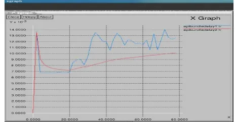
The below figure tells the bundle delay required to reach the destination. Here pure epidemic’s delay is completely random in state where as the Enhanced Epidemic is not random and its delay value is less than pure epidemic’s delay.
Fig: 11 Bundle Delay Comparison between Pure Epidemic (Blue line) & Enhanced Epidemic (Red line)
The packet loss also reduced a lot in enhanced epidemic routing protocol than Pure Epidemic as shown in fig 12.
Fig: 12 Bundle Loss Comparison between Pure Epidemic (Blue line) & Enhanced Epidemic (Red line)
7 CONCLUSIONS
In this paper we conclude that pure epidemic has problems and to overcome that we need to enhance the protocol. The techniques can be implemented are the Anti-packets that manages the buffer level when the buffer size is more, the EC deals with discarding of bundles in the situation when the buffer was filled and no more space for new bundles. The TTL deals with how much time the bundles can alive in the nodes buffer even though there is no Anti-packets received. The combination of EC and TTL can increase more efficiency by changing the TTL value based EC value (when EC crosses threshold then the TTL value will start decreasing) [2].
REFERENCES
[1] Libo Song and David F. Kotz. Evaluating Opportunistic Routing Protocols with Large Realistic Contact Traces.
[2] Feng, Z. & Chin, K. (2012). A unified study of epidemic routing protocols and their enhancements. IPDPSW 2012: IEEE 26th International Parallel and Distributed Processing. Symposium Workshops (pp. 1484-1493).IEEE Explore: IEEE
[3] Morteza Karimzadeh, Efficient Routing Protocol in Delay Tolerant Networks, Topic approved in the computing and Electrical Engineering Faculty Council meeting on 6th April, 2011.
[4] Tim Daniel Hollerung, Peter Bleckmann. Epidemic Algorithms. August 4th ,2004
[5] Ralitsa Kostadinova and Constantin Adam. Performace analysis of Epidemic algorithms.
[6] Harminder Singh Bindra and A. L. Sangal, Performance Comparison of RAPID, Epidemic and Prophet Routing Protocols for Delay Tolerant Networks, International Journal of Computer Theory and Engineering Vol. 4, No. 2, April 2012
[7] Paul Meeneghan & Declan Delaney. An Introduction to NS, Nam and OTcl scripting.