Optimal Power Flow in Shipboard
Power Systems by Differential
Evolution Method
Pedada Puneetha, K.Vaisakh
P.G. Student, Department of Electrical and Electronics Engineering, Andhra University College of Engineering, Visakhapatnam, Andhra Pradesh, India
Professor, Department of Electrical and Electronics Engineering, Andhra University College of Engineering, Visakhapatnam, Andhra Pradesh, India
ABSTRACT: This paper proposes a Differential Evolution Algorithm, for optimal power flow in Shipboard Power Systems with an integrated Photo Voltaic Power Generation Systems. The formulation of Optimal Power Flow problem includes the active power generation and the voltage magnitude at PV buses are considered as control variables. To maintain grid voltage static stable. Modern shipboard power systems of surface vessels acquire efficient and accurate power flow solutions. An assessment of various classical power-flow methods is conducted for shipboard power systems to obtain the power flow solution. In this paper an evolutionary optimization technique called Differential Evolution (DE) algorithm is used for obtaining the power flow calculation problem of integrated shipboard power system. The optimal power flow problem is solved by using Differential Evolution(DE) algorithm considering a objective function and equality and inequality constraints. Case studies of a shipboard power system network demonstrate the introduced methodology succeeds in being the effective one with good convergence on integrated shipboard power system. An evolutionary computation technique is presented, which enhances the computation time and solution convergence.
KEYWORDS: Shipboard power system, Differential Evolution algorithm, optimal power flow. I. INTRODUCTION
In the recent initiatives to update large shipboard power systems, builders of ships are integrating new technologies with the aim of an integrated shipboard power system, i.e., an all-electric energy system. New control strategies utilizing power system automation and reconfiguration of network provide quality of service, reliability, and greater flexibility. These automated controls acquire accurate and efficient power flow solutions [1]. Moreover, power flow calculation problem is the key and foundation of static voltage analysis. Thus, the role of power flow calculation for shipboard power system and the importance is greatly increasing for real-time computation, communication and data control.
methods such as Newton-Raphson are used for shipboard power system. Newton-Raphson can be used in power system with high X/R radios as well as voltage level. While, how to handle PV node is difficult for Forward-Backward sweep method.
Based on the above observation, attention drawn in this paper is to propose a new methodology, i.e., DE algorithm, to solve power flow problem of shipboard power system. DE is one of the evolutionary computation (EC) techniques. The method is improved and applied to various problems[7]. Therefore, DE can be applicable to the problem. The presented technique provides: 1) a new fitness function based on Kirchoff Current Law which makes the initialized variables legal; 2) a novel methodology which reduce variables of bus voltage magnitude and angle on the same branch; 3) a mechanism without dealing with PV node specially.
Renewable energy sources, such as photovoltaic energy systems have been increasingly integrated into shipboard power systems and the applications of renewable energy sources has become a global trend. The photovoltaic energy systems on shipboard power systems are installed to generate electricity and it is further used to supplement the diesel generators so it can reduce the power required from these diesel generator units. The photovoltaic energy systems are included into the optimal power flow model of shipboard power system to minimize the cost and losses in the system.
The paper is organized as follows: .Section II presents the literature survey of the work represented in the paper. Section III elaborates on the features of shipboard power system and the issues associated with it. A general description of calculation of solution of power flow problem for shipboard power system is introduced in Section IV. The overview of DE algorithm that is used in this paper and the illustration of detailed computational flow combined with characteristics of power flow calculation for shipboard power system are briefly stated in Section V. In Section VI, optimal power flow solution for shipboard power system including solar PV systems is explained. Major contributions, and numerical results are presented along with detailed discussion are summarized in Section VII. Finally Section VIII gives the conclusion of the paper.
II. LITERATURE SURVEY
The load flow study in a power system constitutes a study of paramount importance. The study reveals the electrical performance and power flows (real and reactive ) for specified condition when the system is operating under steady state. Besides giving real and reactive the load flow study provides information about line and transformer loading (as well as losses) throughout the system and voltages at different points in the system for evaluation and regulation of power systems. Further study and analysis of future expansion, stability and reliability of the power system network can be easily analyzed in[1]. In this paper the author explains the different load techniques used for load flow study under different specified conditions.
Load flow analysis with one of the most widely used technique Newton Raphson method was explained by the author in [2]. In this paper the author explains the analysis of the technique by comparing it with different iterative techniques. Whereas author in [4] applied the load flow analysis to shipboard power system and obtained the results. Various power flow solution methods like Newton-Raphson method and Fast decoupled method have also been applied to shipboard power systems and their performance is explained in[6].
III. SHIPBOARD POWERSYSTEMS
Most ships today use three-phase, radial systems for service and hospitality loads. These particular systems generate and distribute electric power using an ungrounded delta configuration enabling the power system to be in continuous operation in the event of a single-phase-to-hull fault. Future ships will use electric power systems for virtually all loads and operations [1].Newer ships may also be integrated with either zonal or ring-bus topologies, which form weakly meshed networks[2].
The main advantage of using shipboard power systems is the flexibility to shift power between the mission-critical loads and propulsion as needed. Because the prime mover is further no longer will be tied to the propeller shaft line, the generated power can be real located and distributed throughout the ship. The modularity of the electric system increases flexibility and helps to accomplish rapid reconfiguration of the vital ship systems in the event of network fault damage or when new equipment is introduced. The challenges for calculating the ship power-flow solution quickly depend on utilizing the peculiar system characteristics of the network. Many of these characteristics are common to utility distribution networks:
• weakly meshed network structure; • small ratios in the line impedance; • distributed generation and energy storage • Other characteristics of ship systems:
•
4
G G G G
1 2 8 9 7 5 10 11 12 13 14 15 3 6 16 17 18
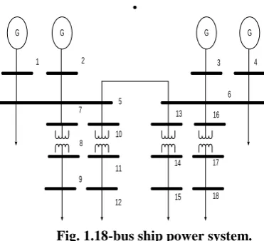
Fig. 1.18-bus ship power system.
• generation that is closely sized to the load demand (i.e., no significant spinning reserve) • a small group of loads that constitute most of the load demand (e.g., the propulsion motors) • short line segments with very low impedance.
Fig. 1 represents the one-line diagram of a typical ship distribution system. In this power network, four variable-speed propulsion drives makeup the four largest loads. Four generators provide the primary power.
IV. POWER FLOWS SOLUTIONMETHOD
Because of the unique characteristics found in medium- voltage radial distribution networks, various distribution power-flow methods have been investigated over the past thirty years [6].Work in distribution power flow has resulted in several techniques in common use today, including the for- ward–backward updating and the bus-impedance matrix forms of the power-flow calculations using linear network equations. These methods typically assume a weakly meshed topology and a single power source[7].
The properties of low-voltage ship distribution networks often render the classical techniques, such as the fast-decoupled method, unsuitable or inefficient. One must exhibit caution when applying even the linear distribution power-flow methods to insure compatibility with short feeder lines and multiple generators. The family of commonly used utility solutions includes the Gauss-Seidel, Newton–Raphson, and fast-decoupled methods.
The Newton Raphson methodology is the most widely used load flow method due to its various advantages. Comparing to alternative processes it has powerful convergence characteristics[19].As computer storage requirements are moderate and increase with problem size almost linearly the NR approach is almost mostly useful for large networks. For a good starting condition this method is very sensitive. To ensure the convergence as well as to reduce the computation time remarkably, the use of a suitable starting condition is required. The effort required for network modifications is quite less computing.
The Newton Raphson methodology has great flexibility and generality, therefore enabling a broad range of representational requirements is to be included efficiently and easily, such as on load tap-changing and phase shifting devices, interchanges in areas, functional loads and voltage remote control. The Newton Raphson approach is central to many recently proposed methods for the optimization in operation of power system, sensitivity analysis system-state estimation, linear-network modeling, evaluation in security and analysis in transient-stability and it is perfectly set to the online computation[9].
To apply the Newton-Raphson method to the problem solution of the power flow equations for a n-bus system in terms of bus admittance matrix Y as:
𝐼𝑖 = 𝑛𝑗 =1𝑌𝑖𝑗𝑉𝑗 (1)
where i, j are to denote ith and jth bus. Expressing in polar form as:
𝐼𝑖 = 𝑛𝑗 =1 𝑌𝑖𝑗 𝑉𝑗 ∠𝜃𝑖𝑗 + 𝛿𝑗 (2)
The current can be expressed in terms of the active power generation and reactive power generation at bus i as:
𝐼𝑖 = 𝑃𝑖−𝑗 𝑄𝑖
𝑉𝑖∗ (3)
Substituting for
I
i from equation (3) in equation (2):𝑃𝑖− 𝑗𝑄𝑖 = 𝑉𝑖 ∠ − 𝛿𝑖 𝑛𝑗 =1 𝑌𝑖𝑗 𝑉𝑗 ∠𝜃𝑖𝑗 + 𝛿𝑗 (4)
Separating the real and imaginary parts:
After calculating the real power and reactive powers we should go for the calculation of power mismatch which is the difference of scheduled power and calculated power and it is expressed as:
∆𝑃𝑖 = 𝑃𝑖,𝑠𝑐ℎ − 𝑃𝑖,𝑐𝑎𝑙 (7) ∆𝑄𝑖 = 𝑄𝑖,𝑠𝑐ℎ − 𝑄𝑖,𝑐𝑎𝑙 (8)
Expanding equations(5) and (6) in Taylor's series about the initial estimate neglecting higher order terms, we get the Jacobian matrix which gives the linearized relationship between small changes in ∆𝛿𝑖(𝑘)and voltage magnitude ∆[𝑉𝑖(𝑘)]
with the small changes in real and reactive power ∆𝑃𝑖(𝑘)and ∆𝑄𝑖(𝑘).
∆𝑃 ∆𝑄 =
𝐽1 𝐽3 𝐽2 𝐽4
∆𝛿
∆ 𝑉 (9)
Using the values of power mismatch and the Jacobian matrices, ∆𝛿𝑖 𝑘
and ∆[𝑉𝑖 𝑘
] are calculated from the equation (9) to complete the particular iteration and the new values for the next iteration can be calculated as
𝛿𝑖(𝑘+1)= 𝛿𝑖(𝑘)+ ∆𝛿𝑖(𝑘) (10)
𝑉𝑖(𝑘+1) = 𝑉𝑖(𝑘) + ∆ 𝑉𝑖(𝑘) (11)
V. OPTIMAL POWER FLOW BY DIFFERENTIAL EVOLUTION METHOD
The optimal power flow (OPF) problem solution aims for optimizing a selected objective function satisfying various equality and inequality constraints and meanwhile via optimal adjustments of power system control variables. Mathematically, the problem of OPF can be formulated as
Min J(x,u) (12) Subject to : g(x,u)=0 (13) h(x,u)≤0 (14) where J is the objective function to be minimized which is expressed as :
𝐹 𝑃 = 𝑁𝐺𝑖 (𝛼𝑖+ 𝛽𝑖𝑃𝐺𝑖+ 𝛾𝑖𝑃𝐺𝑖2) (15)
where α, β, γ are the cost coefficients and NG is number of generators. x is the vector of dependent variables (state vector) consisting of: 1. Generator active power output at slack bus 𝑃𝐺1.
2. Load bus voltage 𝑉𝐿.
3. Generator reactive power output 𝑄𝐺.
Hence, x can be expressed as:
𝑥𝑇 = [𝑃
𝐺1, 𝑉𝐿1… 𝑉𝐿𝑁𝐿, 𝑄𝐺1… 𝑄𝐺𝑁𝐺, 𝑆𝑙1… 𝑆𝑙𝑛𝑙] (16)
where, NL, NG and NL are the number of load buses, number of transmission lines and number of generators, respectively.
u is the vector of independent variables (control variables) consisting of: 1. Generation bus voltage 𝑉𝐺.
2. Generator active power output 𝑃𝐺 at PV buses except at the slack bus 𝑃𝐺1.
3. Transformer tap setting T. 4. Shunt VAR compensation 𝑄𝑐.
Hence, u can be expressed as:
𝑢𝑇 = [𝑃
𝐺2… 𝑃𝐺𝑁𝐺, 𝑉𝐺1… 𝑉𝐺𝑁𝐺, 𝑄𝐶1… 𝑄𝐶𝑁𝐶𝑇1… 𝑇𝑁𝑇] (17)
where NT NC are the number of regulating transformers and VAR compensators, respectively. g these are the equality constraints, which represent typical load flow equations:
𝑃𝐺𝑖− 𝑃𝐷𝑖 − 𝑉𝑖 𝑁𝐵𝐽 =1𝑉𝑗 𝐺𝑖𝑗cos 𝛿𝑖− 𝛿𝑗 + 𝐵𝑖𝑗sin 𝛿𝑖− 𝛿𝑗 = 0
(18)
𝑄𝐺𝑖− 𝑄𝐷𝑖 − 𝑉 𝑁𝐵𝐽 =1𝑉𝑗 𝐺𝑖𝑗sin 𝛿𝑖− 𝛿𝑗 − 𝐵𝑖𝑗cos 𝛿𝑖− 𝛿𝑗 = 0
(19)
where NB is the number of buses, 𝑃𝐺 is the active power generation,, 𝑄𝐺 is the reactive power generation 𝑃𝐷 is the
active load demand,𝑄𝐷 is the reactive load demand 𝐺𝑖𝑗 and 𝐵𝑖𝑗 are the conductance and susceptance between bus i and j
respectively.
h these are the inequality that include: 1. Generator constraints:
Generation bus voltages, active power outputs and reactive power outputs are restricted by their lower and upper limits as:
𝑉𝐺𝑖𝑚𝑖𝑛 ≤ 𝑉𝐺𝑖≤ 𝑉𝐺𝑖𝑚𝑎𝑥, 𝑖 = 1, . . . , 𝑁𝐺 (20) 𝑃𝐺𝑖𝑚𝑖𝑛 ≤ 𝑃
2. Transformer constraints:
Transformer tap settings are restricted by their lower and upper limits as:
𝑇𝑖𝑚𝑖𝑛 ≤ 𝑇𝑖 ≤ 𝑇𝑖𝑚𝑎𝑥, 𝑖 = 1, . . . , 𝑁𝑇 (23)
3. Shunt VAR constraints:
Shunt VAR compensations are restricted by their limits as:
𝑄𝐶𝑖𝑚𝑖𝑛 ≤ 𝑄
𝐶𝑖 ≤ 𝑄𝐶𝑖𝑚𝑎𝑥, 𝑖 = 1, . . . , 𝑁𝐶 (24) A. DIFFERENTIAL EVOLUTION
Recently an evolutionary optimization technique have been proposed to overcome the limitations of classical optimization techniques in solving the optimal power flow(OPF) problem. Various types of heuristic optimization techniques have been proposed such as genetic algorithm(GA), simulated annealing(SA), tabu search, and particle swarm optimization(PSO).
A new floating point encoded evolutionary algorithm is proposed in 1995 by K.Price and R.Storn and it was named as differential evolution (DE) algorithm for global optimization owing to a different kind of differential operator, where they invoked to create new off-spring from parent chromosomes instead of classical crossover or mutation. Differential Evolution (DE) algorithm is a algorithm which is a population based algorithm that uses crossover, mutation and selection operators which is similar to GA to obtain the solution. The Differential Evolution Algorithm is named as self-adaptive due to its selection process and the mutation schemes which are the main differences between GA and DE algorithm. The Differential Evolution algorithm is inspired from the sociological motivations and biological motivations and it is capable on taking care of optimality on, discontinuous, rough and surfaces which are multi-modal. The main advantages of DE are: regardless of the initial parameter values used in DE the near optimal solution can still be found, the characteristics of convergence is fast and it only uses few control parameters. In addition, as DE can handle both integer and discrete optimization which is another task and it is simple in coding, which is easy to use.
B. DE COMPUTATIONAL FLOW
The main features of the DE algorithm can be stated as follows:
1. Like any other evolutionary optimization technique, DE approaches with a population size of NP individuals are D-dimensional variable vectors.
2.Thediscrete time steps of subsequent generations will be represented by 𝑡 = 0,1,2, … , 𝑡, 𝑡 + 1,etc
3.Since the vectors are expected to change over different generations, the following changes may be adopted for representing the ith vector of the population at the current generation (i.e. at time t):
𝑋𝑖
𝑡 = [𝑥𝑖,1 𝑡 , 𝑥𝑖,2 𝑡 , . . . . , 𝑥𝑖,𝐷 𝑡 ] (25)
This vector is referred to as 'genome', 'individual' or 'chromosome'.
(a) differentiation (or mutation) constant F, (b) crossover constant CR, and
(c) population size NP.
(d) dimension of problem D that scales the difficulty of the optimization task;
(e) maximal number of generations (or iterations) GEN, which may serve as a stopping condition; (f) low and high boundary constraints of variables that limit the feasible area.
C. DE ALGORITHM OPERATION
Differential evolution works through a simple cycle of stages presented in figure.2.
Mutation Differential Operator Initialization of Individuals
Selection Crossover
Figure 2. Differential evolution cycle of stages
The major stages of Differential Evolution algorithm can be described as:
D.INITIALIZATION
At the early stage of DE search, i.e., 𝑡 = 0 , the independent variables of problems are initialized somewhere in their feasible numerical range. Therefore, if the jth variable has its lower and upper bounds as 𝑥𝑗𝐿and 𝑥𝑗𝑈, respectively, then
the jth component of the ith population member may be initialized as:
𝑥𝑖,𝑗 0 = 𝑥𝑗𝐿+ 𝑟𝑎𝑛𝑑 0,1 . (𝑥𝑗𝑈− 𝑥𝑗𝐿) (26)
where rand(0,1) is a uniformly distributed random number between 0 and 1.
E. MUTATION
In each generation, a donor vector 𝑣 (𝑡)𝑖 is created in order to change the population vector member𝑋 (𝑡)𝑖 . Generally,
the method of creating this donor vector demarcates between various DE schemes.
1. Three different members 𝑥𝑟1, 𝑥𝑟2 𝑎𝑛𝑑𝑥𝑟3 are chosen randomly from the current population and not coinciding with
the current member 𝑥𝑖.
2.Next, a scalar number F scales the difference between any two of the chosen members and this scaled difference is added to the third one. Therefore, the jth component of 𝑣 (𝑡)𝑖 can be expressed as
𝑣𝑖,𝑗 𝑡 + 1 = 𝑥𝑟1,𝑗 𝑡 + 𝐹(𝑥𝑟2𝑗 𝑡 − 𝑥𝑟3,𝑗 𝑡 ) (27)
This creates the donor vector 𝑣 (𝑡)𝑖 . Typical value of F is in the range of 0.4-1.0. F.CROSSOVER (OR) RECOMBINATION
To increase the diversity of the population, crossover operator is carried out in which the donor vector exchanges its components with those of the current member𝑋 (𝑡)𝑖 .
Moreover, in the case of exponential crossover one has to be aware of the fact that there is a small range of CR values (typically [0.9, 1]) to which the DE is sensitive. This could explain the rule of thumb derived for the original variant of DE. On the other hand, for the same value of CR, the exponential variant needs a larger value for the scaling parameter F in order to avoid premature convergence.
The recombination scheme can be expressed as:
𝑢𝑖,𝑗 𝑡 =
𝑣𝑖.𝑗 𝑡 𝑖𝑓𝑟𝑎𝑛𝑑 0,1 < 𝐶𝑅 𝑥𝑖,𝑗 𝑡 𝑖𝑓𝑟𝑎𝑛𝑑 0,1 > 𝐶𝑅
(28)
𝑢𝑖,𝑗(𝑡)represents the child that will compete with the parent 𝑥𝑖,𝑗(𝑡). G.SELECTION
To keep the population size constant over subsequent generations, the selection process is carried out to determine which one of the child and the parent will survive in the next generation, i.e., at time 𝑡 = 𝑡 + 1. The selection process can be expressed as:
𝑋𝑖
𝑡 + 1 = 𝑈 𝑡 𝑖𝑓𝑓(𝑈𝑖 𝑡 ) ≤ 𝑓(𝑋𝑖 𝑡 )𝑖 𝑋𝑖
𝑡 𝑖𝑓𝑓 𝑋 𝑡 < 𝑓 𝑈 𝑡 𝑖
(29)
where f() is the function to be minimized. So, if the child yields a better value of the fitness function, it replaces its parent in the next generation; otherwise, the parent is retained in the population. Hence the fitness function remains constant but never deteriorates in terms of the population.
VI. OPTIMAL POWER FLOW USING SOLAR PV SYSTEM
able to identify the global optimum. To overcome these drawbacks and handle such difficulties various optimization techniques are developed that are efficient.
To overcome the drawbacks of classical optimization techniques, recently evolutionary optimization techniques have been used to solve problem of Optimal Power Flow solution. A wide variety of heuristic optimization techniques have been applied such as genetic algorithm (GA), simulated annealing (SA), tabu search, and particle swarm optimization (PSO). The results presented in the literature were giving scope for further research in this direction.
Recently an evolutionary optimization technique have been proposed to overcome the limitations of classical optimization techniques in solving the optimal power flow(OPF) problem. The Differential Evolution algorithm is inspired from the sociological motivations and biological motivations and it is capable on taking care of optimality on, discontinuous, rough and surfaces which are multi-modal. The main advantages of DE are: regardless of the initial parameter values used in DE the near optimal solution can still be found, the characteristics of convergence is fast and it only uses few control parameters. In addition, as DE can handle both integer and discrete optimization which is another task and it is simple in coding, which is easy to use .
A photovoltaic system, also PV system or solar power system, is a power system designed to supply usable solar power by means of photovoltaics. Designing effective and reliable PV systems requires understanding both the art and science of photovoltaics and applying the skills, strategies and techniques necessary to meet specific design goals and objectives.
Without doubt the last decade was the golden age of the photovoltaic systems. Solar panels on ships will consist of several solar panels creating one large system. The efficiency of the module represents the conversion of the energy in the light hitting the surface of the module to electricity at its output. The solar panels on ships are installed to produce electricity and will be used to supplement the diesel generators and thus reduce the power required from these units. The solar power units can produce energy both at sea and in port, but only during daylight and therefore the solar panels are set to only produce power 50% of the time. Moreover, solar panels produce power also in cloud cover though not at full capacity.
The solar panel technology is expected to become less expensive over time, but the panels are unlikely to become much more efficient or less space consuming. The cost of solar modules themselves has dropped considerably over time. They are presently approximately Rs 43 per watt of installed capacity. A solar system requires additional equipment beyond the modules. This includes cables, inverters ( to convert DC power to AC power) and the mounting structure. An installation of 1MW would cost upto 450 lakhs. This value is expected to decrease over time, based on what has been seen for land based installations. The estimated reduction potential for solar panel is 0.5% to 2% on auxiliary engine fuel consumption.
The photovoltaic technology can indeed be a really cost-effective solution for ships. PV systems can act as ideal subsidiary power sources, independent from the ship electromechanical settlement because they
(i)produce electric power without the need of transferred gas or liquid fuel, (ii)have no by-products such as gas emissions or noise,
(iii)have low maintenance cost,
(iv)have limited or no use of mechanical moving parts,
(v)consist of few parts, with easy installation and fast replacement in case of aging or defectiveness,
less than the 80% of the nominal one after 25 years of operation,
(vii)can be placed in small surfaces with no practical use such as roofs, walls, funnels, and superstructure,
When we look at point of load, while the load is constant in a solar PV power plant on land, the load on board is mobile according to situation of ship such as anchoring, during voyage, maneuvering etc. While solar radiation data is fixed for solar PV power plant on land, solar radiation data is variable on board. Because generally one ship departure from one port and arrival to other port and after generally do not come back same port where it was departure. During to that different routes, parameters such as latitude, declination angle which are directly affect to generation power from solar panels, change. Because the ship's mechanism is a mobile mechanism and because the load is variable, the influence of the external factors on the panels which are cloudy days, sea water hit, salt, allows the system should be designed more reliable more than power plants on land.
The procedure for implementing optimal power flow in ship power system with solar PV system is given below: Step 1: Run the load flow for ship power system using Newton Raphson method.
Step 2:Run the optimal power flow using Differential Evolution algorithm and store the optimal values of the control variables.
Step 3: Obtain the values for all random variables such as active and reactive power injections.
Step 4: Obtain all the values of output variables such as voltages, line flows and voltage stability index.
Step 5: In case-1, considering the injection of 1MW solar power generation, obtain the values of cost, line flows, voltages and line losses.
Step 6: In case-2, considering the injection of 2MW solar power generation, obtain the values of cost, line flows, voltages and line losses.
VII. NUMERICAL RESULTS
Table 1: Bus data of 18-bus shipboard power system Bus
Number
Bus Type
Voltage Magnitude
(p.u)
Voltage Angle (degrees)
PG
(MW)
QG
(MVAR)
PL
(MW)
QL
(MVAR)
Table 2: Line data of 18-bus shipboard power system Start
Bus
End Bus
Branch Type Branch Resistance(p.u)
Branch Reactance(p.u)
Transformer Tap 1 5 L 0.000167 0.000208 0.00 2 5 L 0.000151 0.000188 0.00 3 6 L 0.000156 0.000195 0.00 4 6 L 0.000162 0.000202 0.00 5 6 L 0.000066 0.000082 0.00 5 7 L 0.000249 0.000310 0.00 5 10 L 0.000172 0.000215 0.00 6 13 L 0.000345 0.000430 0.00 6 16 L 0.000287 0.000358 0.00 7 8 T 0.020563 0.321594 1.00 8 9 L 0.000237 0.000408 0.00 10 11 T 0.020563 0.321594 1.00 11 12 L 0.000237 0.000408 0.00 13 14 T 0.020563 0.321594 1.00 14 15 L 0.000292 0.000502 0.00 16 17 T 0.020563 0.321594 1.00 17 18 L 0.000274 0.000470 0.00
Table 3: Investment Model for 1MW Solar Plant Capacity of Power Plant 1MW
Generation per year 17.50 Lakhs Degradation 1st 10 years 0.05% Degradation 11 to 25 years 0.67% Cost of Electricity per unit Rs. 6.49
Investment Cost per MW 450 Lakhs Operation and Maintenance cost per
year
Case-1
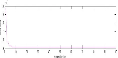
Figure 3. Convergence of cost function using DE
Figure 4. Convergence of fitness function using DE
Case-2
Figure 6. Convergence of fitness function using DE with Solar
Case-3
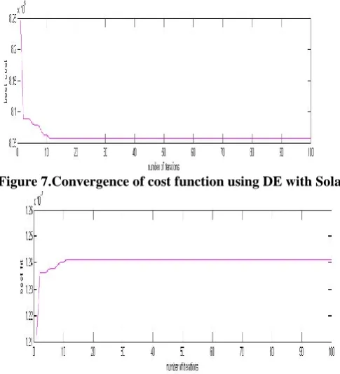
Figure 7.Convergence of cost function using DE with Solar
Case-4
Figure 9. Convergence of cost function using DE with Solar
Figure 10. Convergence of fitness function using DE with Solar
Figure 11.Bar Diagram of Parameters of the Optimal Power Flow Solution 0
0.2 0.4 0.6 0.8 1 1.2
Case-1 Case-2 Case-3 Case-4
Voltage
Power Loss
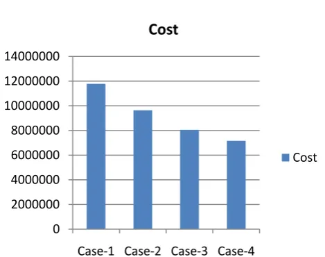
Figure 12. Bar Diagram of Generation costs in Different Cases
The proposed optimal power flow method which uses solar PV system tested on 18-bus shipboard power system. The bus data and line data used for load flow is provided in table-1. The cost coefficients are given in table(4.1). The values of active power generations and voltages are given in p.u. For this shipboard power system different objectives are considered such as minimizing the cost, improving the voltage profile and also considering the control variables such as real power P, voltage V, and tap setting of transformer T are considered and the remaining control variable such as reactive power supplied by shunt compensators are kept constant. Initially several runs are done with different values of DE key parameters such as differentiation(or mutation) constant F, crossover constant CR, size of population NP, and maximum number of generations GEN which is used here as a stopping criteria. The following values are selected as:
F=0.9; CR=0.5; NP=40; GEN=100
Considering the solar power generation the values of voltages, cost, line flows and line losses are tabulated(6)and (5).Convergence characteristics of cost function and fitness function are observed.
From the solution of optimal power flow using DE and the convergence characteristics are shown in (3) and (4). In case-2 Solar PV System is included into the shipboard power system to observe its performance on the system and the results of the optimal power flow using DE with Solar PV System is tabulated. In case-3 the capacity of the Solar PV System is increased compared to the capacity in case-2 and the convergence characteristics are shown (1.7) and( 8). In case-4 the capacity of the Solar PV System is increased compared to the capacities in case-2 and case-3 and the voltage magnitude, power loss, line stability index and cost of the system are tabulated. By including the Solar PV System into the shipboard power system the cost of the system is increased in every case and there are no deviations in the voltage magnitude and the power losses are also reduced in the system.
0 2000000 4000000 6000000 8000000 10000000 12000000 14000000
Case-1 Case-2 Case-3 Case-4
Cost
Table 5 Results of optimal power flow using DE including solar PV system Bus Number Voltage
Case-1 Case-2 Case-3 Case-4 1 0.9724 1.1000 1.1000 1.0449 2 0.9500 1.1000 0.9798 1.0412 3 1.0022 0.9574 0.9500 1.0210 4 0.9758 1.0733 1.1000 1.0438 5 0.9705 1.0690 1.0311 1.0391 6 0.9789 1.0436 1.0269 1.0359 7 0.9702 1.0688 1.0309 1.0389 8 1.0511 1.0356 0.9926 1.0895 9 1.0509 1.0355 0.9925 1.0894 10 0.9703 1.0688 1.0309 1.0390 11 1.0518 1.0363 0.9934 1.0903 12 1.0517 1.0362 0.9933 1.0903 13 0.9785 1.0433 1.0266 1.0357 14 1.0614 1.0098 0.9888 1.0864 15 1.0612 1.0097 0.9887 1.0863 16 0.9786 1.0434 1.0267 1.0358 17 1.0678 1.0149 0.9923 1.0880 18 1.0677 1.0148 0.9922 1.0880
𝑃𝑙 0.3336 0.2510 0.1410 0.0898 𝐿𝑗 0.1681 0.1508 0.1249 0.0909
VIII. CONCLUSION
A method has been proposed for obtaining the power flow solution which is Newton Raphson method has been successfully applied to solve high voltage transmission systems and this method is based on solving the Kirchoff's nodal current equation and this method is tested on the shipboard power system to find the accurate power flow solution that gives the results of voltage magnitude, voltage angle, real power, reactive power, line flows and line losses in the system. The Newton Raphson method is the most reliable and takes the least number of iterations and convergence is not sensitive to the choice of slack bus. In Newton Raphson method, the convergence is fast and the number of iterations is independent of the size of the system, solution to a high accuracy is obtained.
The OPF problem is an optimization problem with in general non convex, non-smooth, and non-differentiable objective functions. It becomes essential to develop optimization techniques that are efficient to overcome these drawbacks and handle such difficulties. An optimization algorithm has been proposed and applied to the optimal power flow problem to obtain the solution. The Differential Evolution has been proposed, developed and successfully applied to solve optimal power flow problem. The optimal power flow problem has been formulated has a constrained optimization problem where several objective functions have been considered to minimize the cost, and to improve the voltage profile. The Differential Algorithm approach has more effectiveness and superiority over the classical and heuristic techniques in terms of solution quality.
A Solar PV system is included into the OPF model in the shipboard power system to reduce the cost and to minimize the deviations in the voltage and to reduce the power loss in the system. The total cost decreases compared to the total cost obtained from the optimal power problem solution using Differential Evolution Algorithm. Solar PV system technologies are playing a major playing role in the applications of ships. The PV systems must be tolerant to special marine environmental conditions and especially the wind, humidity, shading, corrosion problems. The type of cells that are used in the Solar PV system also play major in the cost and also efficiency of the system. The solar panels on ships are installed to produce electricity and will be used to supplement the diesel generators and thus reduce the power required from these units.
REFERENCES
[1] John J. Grainger and Stevenson .W .D., 'Power System Analysis', McGraw Hill, 1st Edition 2003.
[2] Wang, C., Liu, Y., Pan, X.X, 'Load Flow Calculation Of Integrated Shipboard Power System Based On Particle Swarm Optimization Algorithm'. In: Proceedings of the International Conference on Test and Measurement, ICTM 2009.
[3] Glykas, A. Papaioannou, G. Perissakis, S., 'Application and Cost-Benefit Analysis of Solar Hybrid Power Installation on Merchant Marine
Vessels', Ocean Engineering, Vol. 37, pp. 592-602, 2010.
[4] Wu Jishun, HouZhijian (2000). 'The Load Flow Calculation Methods for Shipboard Power Systems on Computer'. Shanghai Jiao Tong University Press, Shanghai, 156- 159.
[5] C.H. Liang, C.Y. Chung, K.P. Wong, X.Z. Duan, C.T. Tse, 'Study of Differential Evolution for Optimal Reactive Power Flow', IET Generation
Transmission and Distribution 1(2) (2007) 253-260.
[6] Zhenyu Yang, Ke Tang, Xin Yao, 'Differential Evolution for High-Dimensional Function Optimization Problem', IEEE Congress on Evolutionary Computation (CEC 2007) 3523-3530.
[7] J.V. Amy Jr, 'Considerations In the Design Of Naval Electric Power Systems'. In: Proceedings 2002 IEEE Power Engineering Society Summer Meeting, Vol.1, 2002, pp. 331-335.
[8] V. Miranda, D. Srinivasan, L.M. Proenca, 'Evolutionary Computation in Power Systems', Electrical Power Energy Systems 20(1998) 89-88. [9] J. Vesterstrom, R. Thomsen, 'A Comparative Study of Differential Evolution, Particle Swarm Optimization, and Evolutionary Algorithms on Numerical Benchmark Problems', IEEE Congress on Evolutionary Computation(2004) 980-987.
[10] AmjadAnvari - Moghaddam, TomislavDragicevic, LexuanMeng, Bo Sun, and Josep M. Guerrero, 'Optimal Planning and Operation Management of a Ship Electrical Power System with Energy Storage System'.
[11] HadiSaadat, 'Power System Analysis', Tata McGraw - Hill Education, 2nd Edition, 2002.