Basic Study on Introduction of the Global-scale LCIA Method “LIME-3” into Environmental Accounting of Local Governments

Article

Basic Study on Introduction of the Global-scale LCIA

Method “LIME-3” into Environmental Accounting of

Local Governments

Junya Yamasaki1_{*, Toshiharu Ikaga}2_{, and Norihiro Itsubo}3

1 _{Graduate School of Science and Technology, Keio University, 3-14-1 Hiyoshi, Kohokuku, Yokohama,} Kanagawa 223-8522, Japan

2 _{Faculty of Science and Technology, Keio University, 3-14-1 Hiyoshi, Kohokuku, Yokohama, Kanagawa} 223-8522, Japan; [email protected]

3 _{Faculty of Environmental Studies, Tokyo City University, 3-3-1 Ushikubonishi, Tsuzukiku, Yokohama,} Kanagawa 224-0015, Japan; [email protected]

* Correspondence: [email protected]; Tel.: +81-45-566-1770

Abstract: Environmental accounting should be performed by both private companies and local governments. However, it may be difficult for government agencies to objectively measure their current environmental impact, and there is currently no internationally standardized methodology of environmental accounting for local governments. This study therefore attempts to incorporate life cycle impact assessment (LCIA) into the calculation of environmental loads for administrative

divisions. In LCIA, environmental loads for several impact categories, such as “Climate change”

and “Land use,” are integrated into a simple indicator expressed in terms of monetary units. This study leverages the LIME-3 assessment theory, one of the endpoint-type and global-scale LCIA methods. Annual environmental loads for administrative divisions in 42 countries were measured in a tentative assessment. Results showed that the annual damages for the 42 countries to be USD 10.5 trillion. Assessment results are shown on the world map to highlight the regionality of the

damages in the 42 countries’ administrative divisions. This study seeks to provide new knowledge

that local governments around the world can use in environmental accounting.

Keywords: Environmental accounting; LCIA method; local government; OECD; statistical information

1. Introduction

In recent years, some international frameworks, such as the Sustainable Development Goals (SDGs) and the Paris Agreement, have promoted environmental conservation in countries around the world. It is important for enterprises around the world to decide their environmental policies after carefully examining their own economic circumstances. Enterprises should therefore seek to build consensus on their future paths based on the relationship between the environment and the

economy. In order to provide guidance for these problems, the United Nations published “The

System of Environmental-Economic Accounting (SEEA)” [1], an international standard framework

that integrates economic and environmental information, in 2012. The SEEA contains internationally agreed upon concepts, definitions, classifications, and accounting rules. The SEEA framework follows an accounting structure similar to that of the System of Nation Accounts (SNA). By using this framework, enterprises in each country have been encouraged to manage their own environmental and economic statistics. Against this background, it has become increasingly important that business operators quantitatively measure, recognize, and transfer their own environmental considerations in order to build a sustainable society.

Environmental accounting—a system in which an enterprise reports its environmental

activities quantitatively in monetary terms—is mainly used in private companies, although there are

some examples of local governments which have aggressively introduced this system. For example, the local government of Eurobodalla in Australia publishes annual statistics on the sustention of assets for environmental conservation [2]. The cities of Sabae and Yokosuka in Japan also publish environmental accounting on an annual basis using one-of-a-kind methods [3-4]. These governments struggle to calculate not only environmental costs but also environmental conservation effects, and it is difficult for local governments to measure the environmental value of their own administrative divisions in an objective way. Previous studies have investigated environmental accounting for local governments [5-9], but a global-scale system that includes a comprehensive and quantitative methodology for several environmental categories has not yet been established. Additionally, the SEEA does not describe the scientific methodology for calculating environmental value based on concrete environmental indicators. An international standard of environmental accounting for local governments has therefore not been established, so these systems have not been implemented worldwide.

An important concept in life cycle assessment research is life cycle impact assessment (LCIA), which is the quantitative measurement of environmental impacts throughout the life cycle of products and services. A methodology has been developed whereby the environmental loads of

several impact categories, such as “climate change” and “land use,” are integrated into a simple

indicator. Several assessment methods that include the theory of integration have already been developed, such as ExternE [10], EPS [11], and Eco-indicator 99 [12]. However, there is no nation that officially incorporates this assessment theory into calculations of environmental conservation effects across all governmental agencies for set periods of time. Some studies have used a scientific methodology to assess the environmental impacts of geographic areas, such as areas of countries or

communities; for example, “carbon footprint” and “land footprint” [13-17]. However, standard

systems that comprehensively utilize these research outcomes to measure governmental agencies’

environmental value have not yet been established. It is therefore possible that LCIA may provide useful knowledge that will help in constructing a unified methodology for the environmental accounting of local governments.

This study focuses on local governments, which are governmental agencies closely connected to the livelihood of local residents, and describes the fundamental considerations for introducing LCIA theory into environmental accounting practices. This study leverages the assessment theory of LIME-3 (Life-Cycle Impact Assessment Method Based on Endpoint Modeling 3), which was developed in 2018 [18-25]. This endpoint-type and global-scale LCIA method reflects environmental conditions and environmental sciences from around the world. This includes the integration theory of LCIA and is able to calculate assessment results as monetary units while integrating the environmental loads of several impact categories. In this way, public administrators can specifically compare the policy effects of different categories. This system is expected to contribute to decision-making when choosing investments for assessing environmental conservation by each administrative division. Moreover, governments around the world can measure environmental loads in the same way, which could promote comparative studies and information sharing. For these reasons, this study presents a basic proposal to integrate the assessment theory of LIME-3 into the

calculation of local governments’ environmental conservation effects, and provides tentative

assessments for administrative division in 42 countries, most of which are OECD members. A standard methodology of environmental accounting for local governments was produced using the research results.

2. Summary of Assessment

2.1. Philosophy of Assessment

requirements for local governments’ environmental accounting. (1) Fitness for purpose: environmental accounting must provide useful information for decision-making by administrators. (2) Reliability: environmental accounting must reduce or eliminate serious mistakes and biases in information and inspire confidence in all stakeholders. (3) Clarity: environmental accounting must explicitly display the information required for administrators and prevent them from making incorrect decisions. (4) Comparability: environmental accounting must provide comparable information between periods and between local governments. (5) Verifiability: environmental accounting must provide objectively verifiable information for stakeholders.

Case examples of local governments’ environmental accounting show that these calculated

items can be divided into two main parts: the costs and the effects of environmental conservation. The LCIA can most effectively evaluate the effects; thus, it is the focus of this study. Environmental conservation by local governments is defined as the results of actions that administrators take, such as emission prevention, control and avoidance of environmentally hazardous substances, and recovery from these types of environmental damage. This study uses a basic formula which defines the difference in the total amount of environmental loads between the base period and the current period in an administrative division of the local government. The calculation formula is described as follows.

( )

( )

( )

The effect of environmental consevation

The total amount of environmental loads in base period The total amount of environmental loads in current period

= −

(1)

This study focuses on the total amount of environmental loads for a certain period, as seen in the terms on the right side in Eq. (1), and provides calculation methods for them using the assessment theory of LCIA.

2.2. Summary of LIME-3

This study utilizes LIME-3 to measure the total amounts of environmental loads as described above. LIME-3 has several methods of calculation for different countries around the world and is able to assess environmental impact based on their respective environmental conditions. The assessment framework for LIME-3 is shown in Figure 1. The assessment processes of LIME-3 are divided into two steps, the damage assessment and the integration, and each factor list is provided in order to calculate the results for different assessment purposes. This study aims to calculate assessments as an integrated simple indicator in terms of monetary units; the integration factor lists were used accordingly. The integration factors are provided for each of the following: hazardous substances, impact categories, countries of origin, and safeguard subjects. Incidentally, these factors are calculated as a reflection of the causal relationship between the countries of origin and the affected countries for environmental impact. For example, in regard to air pollution, LIME-3 is able to calculate the results while considering the movement of hazardous substances across borders. The assessment results with the simple indicator converted into a monetary value (USD) are obtained by multiplying these factors with corresponding inventory data and summing these values. The calculation formula is described as follows.

(

)×

(

)

impact X

SI

=

 

Inv X

IF

X

SI : Single indicator [USD] Inv(X) : Inventory of substance X [kg]

IFImpact_{(X) : Integration factor of substance X [USD/kg]}

Inventory NOx SO2 PM2.5 NMVOC CO2 CH4

N2O

Water Oil Natural gas Iron Gold Timber Land Integration Damage assessment Damage factors Air pollution Climate change Water Fossil fuels Mineral resources Forest resources Land use Waste Integration factors Weighting factors (For each country of origin)

(For each country of origin and each endpoint)

Results of damage assessment Human health DALYs Social assets USD Biodiversity EINES Primary production NPP

(Can be classified into countries of origin and affected countries)

(For each country subject to assessment)

(G20, G8 countries, emerging countries) Human health Social Assets Biodiversity Primary production Results of integration

(Can be classified into countries of origin and affected countries) Single indicator Index USD Weighting Air pollution Photochemical oxidant Climate change Water Fossil fuels Mineral resources Forest resources Land use Waste NOx SO2 PM2.5 NMVOC CO2 CH4

N2O

Water Oil Natural gas Iron Gold Timber Land NOx SO2 PM2.5 NMVOC CO2 CH4

N2O

The framework of LIME-3 has nine impact categories, such as “Climate change” and “Air

pollution.” Some environmental hazardous substances, such as CO2 and fine particulate matter

(PM2.5), are used as inventory items in each impact category. The four safeguard subjects, “Human

health,”“Social assets,”“Biodiversity,” and “Primary production,” are shown in the corresponding

impact category. In the LIME-3 framework, the calculated results of 4 safeguard subjects are

weighted by conjoint analysis based on a survey of people’s values through the process of the

integration. This survey targeted residents of G20 countries. Using this, assessment results converted

into monetary value can be calculated as a reflection of each nation’s environmental values.

Moreover, the average integration factors are provided in order to calculate the assessment results under the same conditions throughout the world. Thus, LIME-3 has several calculation procedures for its various assessment purposes.

Showing environmental loads using a simple indicator converted into a monetary value meets

the requirements of “Fitness for purpose” and “Clarity,” which are two of the general requirements

for local governments’ environmental accounting described above. Administrators can gain useful

information about the annual effects of their own activities in each environmental category, which could contribute to decision-making in areas such as allocation of environmental conservation expenses. Easy-to-understand information can be provided to the general public by showing the clear assessment results. In addition, assessment of environmental loads using a single global-scale

method meets the requirement of “Comparability.” Since administrators can compare their

assessment results with those of others, these reports could promote information sharing between local governments in different countries. This may contribute to the search for best practices in environmental activities around the world.

There are other global-scale LCIA methods, such as LC-IMPACT [26], IMPACT World+ [27], and EPS [11]. Based on our requirements, LIME-3 is the most advantageous of the LCIA methods for the assessment of local government policies.

3. Assessment Method

In this section we describe the basic points of the assessment method.

3.1. Assessment Period

The assessment period of this method is defined as the fiscal operating period of the local governments in order to avoid confusion between financial and environmental statistics. This is basically defined as one year, with flexibility to account for the availability of information.

The assessment scope of this method is defined as all sectors, including industry, consumers, transportation and households, since local governments are accountable to a wide range of constituencies within their jurisdictions. Administrators endeavor to ascertain current conditions based on the inventory data divided into as many sectors as possible to allow for practical use of this method.

3.3. Geographical Location of Environmental Impact

Next, we discuss the geographical aspect of environmental impacts. In recent years, it has become necessary to take into consideration the international nature of supply chains when

considering environmental impacts. For example, the framework of “Scope 1, 2, 3” is incorporated

into calculations of greenhouse gas (GHG) emissions. “Scope 1“ targets GHG emissions that are

directly emitted by an enterprise, such as those resulting from the consumption of natural gas and

other fossil fuels. “Scope 2” targets GHG emissions that are indirectly emitted by an enterprise, such

as those resulting from the use of electricity. “Scope 3” targets GHG emissions that are indirectly

emitted by an enterprise through its supply chains, such as production, transportation, and disposal of products used by the enterprise. In LIME-3, every kind of resource consumption can be assessed for imports and exports between countries, but the movement of ready-made products across borders of administrative divisions is necessary to consider by users who prepare the inventory data. Therefore, we must decide how we will treat the movement of ready-made products between administrative divisions. For example, even if a certain local government reduces its annual environmental load, this outcome should not be captured as only the effort of this local government alone, as modern industry and agriculture are connected at the international level and highly specialized within countries.

This study approaches this problem using two ideas, the principle of territorial occurrence and the principle of territorial consumption. The principle of territorial occurrence counts environmental loads from production, consumption, and disposal of any products in the administrative divisions where these actions are carried out and where these loads are incurred. In contrast, the principle of territorial consumption counts environmental loads in the administrative divisions where products are consumed and where someone receives a benefit from them. When a certain product is produced in area A and consumed in area B, the environmental loads related the product are counted in area A under the former principle and in area B under the latter. The relative advantages and disadvantages of these two principles are shown in Table 1.

Table 1. Advantages and disadvantages of the principle of territorial occurrence and the principle of territorial consumption

Principles Advantage Disadvantage

Principle of territorial occurrence

Comparatively easy to prepare required data for assessment

Unable to directly interpret the individual responsibility of a local government based on these assessment results

Principle of territorial consumption

Ability to determine efforts of local governments in assessment results and compare with others

Inventory data for movement of materials between all areas must be considered

development of an assessment method that uses the principle of territorial consumption will be a challenge for the future.

4. Assessment of Administrative Divisions

Using the above-mentioned method, environmental impact assessment of administrative divisions in each country was conducted. The assessment was calculated as a measurement of the total amount of environmental loads for a certain period using Eq. (1) above.

4.1. Targets for Assessment

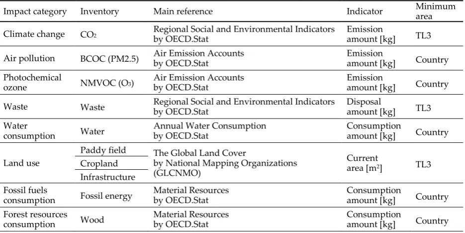
Although the framework of LIME-3 lists inventories by impact category, it may not be easy to prepare all inventory data for the assessment for some assessment targets. Assessment indicators must therefore be selected while considering the purpose of the assessment, data availability, and

data precision. This study focuses on the concepts of “Reliability,” “Comparability,” and

“Verifiability,” which are the general requirements for local governments’ environmental

accountings as stated above. For “Reliability,” we refer to internationally authoritative information

to assess administrative divisions around the world. Second, for “Comparability,” we use inventory

data that is as comparable as possible between countries to effectively compare assessment results.

For “Verifiability,” we refer to information that is widely available to the general public in order to

produce assessment results that can be objectively verified. This study uses these concepts to refer to information that is uniformly compiled and published by international statistics organizations.

As this study focuses on countries who belong to the Organization for Economic Co-operation and Development (OCED), we utilize statistical information published by the statistics bureau of the OECD (OECD.Stat) [28]. This data was used mainly for assessments of administrative divisions. OECD.Stat aggregates data from the statistics bureaus of some countries, most of which are OECD members, and is a reliable source of information because it publishes uniform information about administrative divisions worldwide. In this study, we target 42 countries, of which 35 are OECD members. Data for seven non-OECD countries (Brazil, China, Colombia, India, Lithuania, Russia, and South Africa), for which information is readily available through OECD.Stat was also included. Required data which was unavailable through OECD.Stat was obtained from other international organizations or statistics bureaus in each respective country.

OECD.Stat defines the area classifications for all countries for which it publishes statistics at two territorial levels (TLs), a higher level (TL2) and a lower level (TL3). TLs are defined mainly according to the population of each unit. A TL2 unit consists of some number of TL3 units, and national land consists of some number of TL2 units. This definition is standardized within countries, and territories generally correspond to the administrative divisions of each country. This study therefore defines the area of assessment according to TL. From the perspective of data availability, the minimum area unit of assessment was defined as TL3 units within the 35 OECD countries, and as TL2 units within the 7 non-OECD countries. Additionally, in cases that required data for units that were not available, estimated data was used.

4.2. Preparation of Data

Incidentally, inventory data for “Land use” was taken from data published by the National Mapping Organization (NMO) [29]. All land use data was converted into TL3 units using ArcGIS

(10.5) software. “Land use” in this study is limited to human-made areas, including paddy fields,

cropland, and infrastructure, from the perspective of local government responsibility.

In cases where inventory data was not available by TL2 or TL3 unit, the required data was estimated based on proportionate distribution using other related data. The emission amounts of

each substance, such as CO2 and SO2, were available only by country unit, and emissions in the

industrial sector accounted for most of total emissions. Emission amounts were divided proportionally by TL2 or TL3 unit using data on the number of employees per division. Consumption of water, fossil energy, and wood was also available by country only, with consumption closely related to the lives of the citizenry. Consumption amounts were divided

proportionally by TL2 or TL3 unit using population data. The “Mineral resources consumption”

category was not included in this assessment because of a lack of detailed data and low estimation accuracy.

In this study the average integration factors above were used to unify the weighting of the 4 safeguard subjects for the same condition throughout the world.

4.3. Assessment Results and Discussions

The results of the environmental impact assessment for administrative divisions in 42 countries are described using monetary value as an indicator. This indicator can be interpreted as the annual

amount of damage to the environment in each division. This indicator is called “Damage amount of

environmental impact (USD)” in this study.

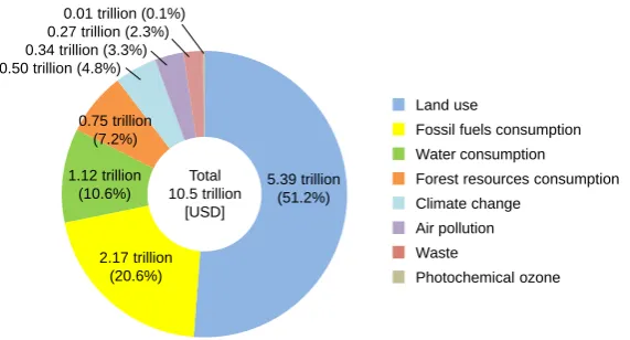
4.3.1. Summation Damage Amount in 42 Countries

First, the summation of damage amount caused in the total area of 42 countries was calculated. The summation by impact category is shown in Figure 2, and the summation for each safeguard subject is shown in Figure 3.

Table 2. Availability of inventory data by each impact category

Impact category Inventory Main reference Indicator Minimum _area

Climate change CO2 Regional Social and Environmental Indicators

by OECD.Stat

Emission

amount [kg] TL3

Air pollution BCOC (PM2.5) Air Emission Accounts _{by OECD.Stat} Emission _{amount [kg]} Country

Photochemical

ozone NMVOC (O3)

Air Emission Accounts by OECD.Stat

Emission

amount [kg] Country

Waste Waste Regional Social and Environmental Indicators _{by OECD.Stat} Disposal _{amount [kg]} TL3

Water

consumption Water

Annual Water Consumption by OECD.Stat

Consumption

amount [kg] Country

Land use

Paddy field _{The Global Land Cover}

by National Mapping Organizations (GLCNMO)

Current

area [m2_] TL3

Cropland Infrastructure Fossil fuels

consumption Fossil energy

Material Resources by OECD.Stat

Consumption

amount [kg] Country

Forest resources

consumption Wood

Material Resources by OECD.Stat

Consumption

amount [kg] Country

The total damage amount was 10.5 trillion USD. In Figure 2, the top three amounts by impact

category were “Land use” (5.39 trillion USD), “Fossil fuels consumption” (2.17 trillion USD), and

“Water consumption” (1.12 trillion USD). The damage amount for “Land use” accounted for 51.2%

of the total, and the top three amounts accounted for 82.7% of the total. In Figure 3, the amounts for

each safeguard subject were “Biodiversity” (5.63 trillion USD), “Social Assets” (2.40 trillion USD),

“Human health” (1.76 trillion USD), and “Primary production” (0.73 trillion USD). In particular, the

damage amount to “Biodiversity” caused by “Land use” accounted for 89.3% of the total amount for

“Biodiversity.” This suggests that human development has a significant impact on Earth’s

biodiversity.

Based on these results we can use the LIME-3 theory to compare the environmental impacts in each impact category and safeguard subject using a single indicator. In recent years, sustainable development has come to be recognized as an issue in a variety of scientific fields. In particular, it has been suggested that efficient utilization of farmland and urban development are extremely important from the perspective of environmental impact.

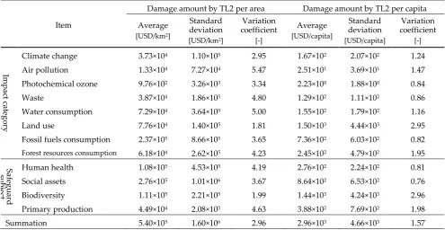
4.3.2. Damage Amount by TL2 unit

The environmental damage by TL2 unit for 42 countries is described in this section. Here, the damage amount per unit area and per capita for each TL2 was calculated. These results are shown in Table 3, which lists the average, standard deviation, and variation coefficient for each impact category and safeguard subject. Coefficient variation is calculated by dividing the standard deviation by the average, and it shows relative variation in the data.

The TL2 averages of total damage amounts per unit area and per capita were calculated as

540,000 USD/km2 _{and 2,960 USD/capita. The top three amounts per area unit by each impact}

category were “Fossil fuels consumption” (237,000 USD/km2_{), “Land use” (77,600 USD/km}2_{), and}

“Water consumption” (72,900 USD/km2_{). The top three amounts per capita by each impact category}

5.39 trillion (51.2%)

2.17 trillion (20.6%) 1.12 trillion

(10.6%) 0.75 trillion

(7.2%) 0.50 trillion (4.8%)

0.34 trillion (3.3%) 0.27 trillion (2.3%)

0.01 trillion (0.1%)

Land use

Fossil fuels consumption

Water consumption

Forest resources consumption Climate change

Air pollution

Waste

Photochemical ozone Total

10.5 trillion [USD]

Figure 2. Total damage amounts of 42 countries by impact category

5.63 trillion (53.5%) Total

10.5 trillion [USD]

2.40 trillion (22.8%) 1.76 trillion

(16.7%) 0.73 trillion

(6.9%)

Biodiversity

Social assets

Human health

Primary production

were “Land use” (1,500 USD/capita), “Fossil fuels consumption” (736 USD/capita), and “Forest

consumption” (245 USD/capita). TL2 unit is mainly defined based on the population size for each

division, but the area of each division varies greatly. Consequently, the magnitude of the relationship of the average damage amount between per area unit and per capita differed accordingly for each impact category.

Next, we will discuss the variation coefficient per area unit and per capita. Each variation

coefficient per capita was smaller than the per area unit for all impact categories except “Land use,”

for all safeguard subjects except “Biodiversity,” and for the summations. This indicates that the per

capita variation was relatively small compared with the per area unit variation. This shows that the trends of these damage amounts were closer to the population size rather than the area size of each division, although it consideration of the effect of the data estimation used above was required. In

contrast, the variation coefficient of “Land use” and “Biodiversity” per area unit was smaller than

that per capita. It showed that the trends of these damage amounts were closer to area size than population size. These results verify the general characteristics of these items.

4.3.3. Regionality of Damage Amount

The assessment results above are shown on a world map to illustrate the regional damage in the administrative divisions in 42 countries. A world map showing damage per area unit and per capita for each TL is shown in Figure 4. The map of Europe is shown in Figure 5. Here, damage for all divisions is shown so that map colors are shown in 10% increments of cumulative frequency distribution. The area unit of description on the map followed the minimum area of assessment as described above, which was TL3 within the 35 OECD countries, and TL2 within the 7 non-OECD countries.

In examining the world map in Figure 4 as a whole, we find that the damage amount per area unit tended to be higher in areas of concentrated population. In particular, the damage tended to be higher in urban areas. On the other hand, the damage amount per capita tended to be higher in sparsely populated areas, although there were some exceptions. As seen above, the trend of both amounts per area unit and per capita were more or less inverted. Detailed trends for each region were diverse, so there are opportunities to reflect on the characteristics of environmental loads within each region. Next, we will look at each region in the world.

(1) North America (Figure 4)

Table 3. Assessment results of damage amount by TL2

Item

Damage amount by TL2 per area Damage amount by TL2 per capita

Average

[USD/km2_]

Standard deviation

[USD/km2_]

Variation coefficient

[-]

Average

[USD/capita]

Standard deviation

[USD/capita]

Variation coefficient

[-]

Im

pa

ct

c

at

eg

or

y

Climate change 3.73×104 _1.10×105 _{2.95 1.67×10}2 _2.07×102 _1.24

Air pollution 1.33×104 _7.27×104 _{5.47 2.51×10}1 _3.69×101 _1.47

Photochemical ozone 9.76×102 _3.26×103 _{3.34 2.23×10}0 _1.88×100 _0.84

Waste 3.87×104 _1.86×105 _{4.80 1.29×10}2 _1.11×102 _0.86

Water consumption 7.29×104 _3.64×105 _{5.00 1.55×10}2 _1.79×102 _1.16

Land use 7.76×104 _1.40×105 _{1.81 1.50×10}3 _4.44×103 _2.95

Fossil fuels consumption 2.37×105 _8.66×105 _{3.65 7.36×10}2 _6.03×102 _0.82

Forest resources consumption _6.18×104 _2.62×105 _{4.23 2.45×10}2 _4.79×102 _1.95

S

afeg

ua

rd

sub

je

ct

Human health 1.08×105 _4.53×105 _{4.19 2.76×10}2 _2.24×102 _0.81

Social assets 2.76×105 _1.01×106 _{3.67 8.64×10}2 _6.53×102 _0.76

Biodiversity 1.11×105 _2.21×105 _{1.99 1.44×10}3 _4.24×103 _2.96

Primary production 4.49×104 _2.08×105 _{4.63 3.88×10}2 _7.69×102 _1.98

Summation 5.40×105 _1.60×106 _{2.96 2.96×10}3 _4.66×103 _1.57

Damage per area unit tended to be higher around the West Coast, East Coast, and Great Lakes regions in the USA, and around Mexico City in Mexico. Because these are some of the most concentrated areas in the world, amounts were comparatively higher. Per capita damage tended to be high over a wide area of North America compared with that in the rest of the world. The fact that large-scale industry and agriculture are widespread in North America, may account for the higher than average per capita amounts.

(2) South America (Figure 4)

Here, damage per area unit was found to be higher around the major cities in each country, such as Rio de Janeiro and São Paulo in Brazil, Bogota in Colombia, and Santiago in Chile. These are densely populated areas, so their damage amounts trended higher. However, per capita amounts were comparatively low around Rio de Janeiro and Bogota. Although these cities have major industries, the per capita amounts may be lower because of their larger populations.

(3) Europe (Figure 5)

In Europe, damage per area unit tended to be higher in areas of concentrated population perhaps reflecting industrial activity. The amounts in England, the Iberian Peninsula, the Benelux countries, western Germany, and the Italian Peninsula were higher than in other areas since these regions are home to major industries. In terms of per capita damage, in some regions the amount was lower in all areas of the country; for example, Switzerland, Austria, Slovenia, Czech Republic, Slovakia, and Hungary. One reason for this was that there are mountainous areas in these regions. Additionally, the amount per area unit was also comparatively lower in Austria, so these results may reflect the higher environmental standards in these countries.

(4) Africa (Figure 4)

Damage per area unit was higher in the urban area of Johannesburg in South Africa. This city is densely populated and has many factories and the results reflect these conditions. Per capita results tended to be higher in sparsely populated areas and lower in densely populated areas such as around Johannesburg and Cape Town, which is consistent with trends in the rest of the world.

(5) Russia and Asia (Figure 4)

Damage per area unit tended to be higher in India and the eastern areas of China, which are among the most densely populated areas in the world. Damage per area unit was also higher in the Republic of Korea and Japan. On the other hand, amounts were lower in eastern Russia and western China, which are sparsely populated areas. Per capita, damage tended to be lower in densely populated areas in contrast to the damage amount per area unit. Although these areas had large environmental loads, the amount per capita was lower because of their larger populations.

(6) Oceania (Figure 4)

Figure 4. Assessment results by administrative division, global

Figure 5. Assessment results by administrative division, Europe Damage amount per unit area

Damage amount per capita

Damage amount per unit area

Damage amount per capita

80% - 90% 90% - 100% 70% - 80% 60% - 70% 50% - 60% 40% - 50% 30% - 40% 20% - 30% 10% - 20% 0% - 10%

( 872,000 - )

( - 27,200) ( - 69,800) ( - 101,000) ( - 138,000) ( - 183,000) ( - 244,000) ( - 342,000) ( - 463,000) ( - 872,000)

Damage per unit area[ USD/km2_]

hi

g

h

low

80% - 90% 90% - 100% 70% - 80% 60% - 70% 50% - 60% 40% - 50% 30% - 40% 20% - 30% 10% - 20% 0% - 10%

( 46,300 - )

( - 1,490) ( - 1,940) ( - 2,140) ( - 2,590) ( - 3,590) ( - 5,820) ( - 10,800) ( - 21,800) ( - 46,300)

Damage per capita[ USD/capita ]

hi

g

h

The results above summarized the environmental loads of 42 countries’ divisions by damage amount per area unit and per capita based on the method described in this paper. This allowed us to study comparatively the current state of the environmental impacts around the world.

As shown by the visualizations on the world maps, the more densely inhabited, the higher the environmental load per area unit tended to be. In contrast, the results suggest that more densely populated areas tended to have lower environmental loads per capita, reflecting greater environmental efficiency.

5. Conclusions

This paper presented a basic study introducing the theory of LCIA into the calculation of environmental loads from administrative divisions in order to provide new information for local governments around the world to use in environmental accounting. Based on the theory of LIME-3, an assessment method of environmental impact for governmental agencies under the assessment

concepts of “Fitness for purpose,”“Clarity,” and “Comparability” was demonstrated. Moreover, the

annual environmental loads for each administrative division in 42 countries were calculated as a preliminary assessment. Here, the availability of required information by administrative divisions was obtained from international statistics organizations and statistics bureaus in each country in

order to prepare inventory data under the assessment concepts of “Reliability,” “Comparability,”

and “Verifiability.” Assessment results were compared and visualized on world maps. As described

in this paper, an elementary framework needed to develop a unified method of environmental accounting for local governments was developed.

Future challenges for this topic include the need to collect more inventory data to improve the reasonability and usefulness of this method. The inventory data used in this study was based on limited statistical information that compared assessment results under the similar conditions around the world. More useful assessment results might be calculated with the cooperation of statistics organizations and research institutions in each country. For example, time-series information is required to calculate the environmental conservation effect of each administrative divisions based on Eq. (1) as above. In addition, more specific statistics are required to calculate assessment results for some sectors, such as industry, consumers, and transportation. Moreover, although this study was limited to describing the assessment results on the world maps above, there is a need to focus on individual cities or metropolitan areas around the world and describe detailed results for each impact category to present the specific practicality of this method. In addition, technical problems should be considered, such as the development of an assessment theory using the principle of territorial consumption discussed above, as well as comparisons with the assessment results calculated by other LCIA methods. Overcoming these challenges would help to create new insights in the field of LCA in the future.

Acknowledgments: This research received no external funding.

Author Contributions: Conceptualization, J.Y.; Methodology, J.Y. and N.I.; Software, J.Y.; Validation, J.Y.; Formal Analysis, J.Y.; Investigation, J.Y.; Resources, J.Y.; Data Curation, J.Y.; Writing – Original Draft Preparation, J.Y.; Writing – Review & Editing, J.Y.; Visualization, J.Y.; Supervision, J.Y.; T.I.; Project Administration, J.Y.

Conflicts of Interest: The authors declare no conflict of interest.

References

1. System of Environmental Economic Accounting. Available online: https://seea.un.org/ (accessed on Dec 24, 2018).

2. Eurobodalla Shire Council, Local Environmental Plans. Available online:

http://www.esc.nsw.gov.au/development-and-planning/tools/local-environmental-plans/ (accessed on Dec 24, 2018).

3. Environmental Accounting of Yokosuka City. Available online:

4. Environmental Report of Sabae City. Available online:

https://www.city.sabae.fukui.jp/kurashi_tetsuduki/sizen/kankyohokokusho/index.html (accessed on Dec 24, 2018).

5. Pim, D.; Nicolas, J.; Jens N. Environmental Accounting and Change in UK Local Government. Accounting Auditing & Accountability Journal2005, 18, 346-373. Available online:

https://www.researchgate.net/publication/242348359_Environmental_accounting_and_change_in_UK_loc al_government (accessed on Dec 23, 2018).

6. Qian, W.; Burritt, R. Contingency Perspectives on Environmental Accounting: An Exploratory Study of Local Government. Accounting, Accountability & Performance2009, 15, 39-70. Available online:

https://search.informit.com.au/documentSummary;dn=011795652420461;res=IELBUS (accessed on Dec 23, 2018).

7. Federica, F.; James, G. Sustainability Reporting by Australian Public Sector Organisations: Why They Report. Accounting Forum2009, 33, 89-98. Available online:

https://www.sciencedirect.com/science/article/pii/S015599820900009X (accessed on Dec 23, 2018).

8. Qian, W.; Burritt, R.; Monroe G. Environmental Management Accounting in Local Government: A Case of Waste Management. Accounting, Auditing & AccountabilityJournal2011, 24, 93-128, Available online: https://www.emeraldinsight.com/doi/abs/10.1108/09513571111098072 (accessed on Dec 23, 2018).

9. Qian, W.; Burritt, R.; Monroe G. Environmental Management Accounting in Local Government: Functional and Institutional Imperatives. Financial Accountability & Management 2018, 34, 148-165, Available online:

https://onlinelibrary.wiley.com/doi/abs/10.1111/faam.12151 (accessed on Dec 23, 2018).

10. ExternE - External Costs of Energy. Available online: http://www.externe.info/externe_d7/ (accessed on Dec 24, 2018).

11. Environmental Priority Strategies (EPS). Available online:

http://www.gabi-software.com/international/support/gabi/gabi-lcia-documentation/environmental-priori ty-strategies-eps/ (accessed on Dec 24, 2018).

12. Eco-Indicator 99. Available online:

http://www.gabi-software.com/international/support/gabi/gabi-lcia-documentation/eco-indicator-99/

(accessed on 24-12-2018).

13. Steven, D.; Ken, C. Consumption-based Accounting of CO2 Emissions. Proc. Natl. Acad. Sci. U. S. A.2010,

107, 5687-5692, Available online:

https://www.pnas.org/content/107/12/5687 (accessed on Dec 23, 2018).

14. Steen-Olsen, K.; Weinzettel, J.; Cranston, G.; Ercin, E.; Hertwich, E. Carbon, Land and Water Footprint Accounts for the European Union: Consumption, Production and Displacements Through International Trade. Environ. Sci. Technol.2012, 46, 10883-10891, Available online:

https://research.utwente.nl/en/publications/carbon-land-and-water-footprint-accounts-for-the-european-union-c (accessed on Dec 23, 2018).

15. Ivanova, D.; Vita, G.; Steen-Olsen, K.; Stadler, K.; Melo, P.; Wood, R.; Hertwich, E. Mapping the Carbon Footprint of EU Regions. Environ. Res. Lett.2017, 12, 1-13, Available online:

http://iopscience.iop.org/article/10.1088/1748-9326/aa6da9 (accessed on Dec 23, 2018).

16. Oppon, E.; Acquaye, A.; Ibn-Mohammed, T.; Koh L. Modelling Multi-regional Ecological Exchanges: The Case of UK and Africa. Ecological Economics2018, 147, 422-435, Available online:

https://www.sciencedirect.com/science/article/pii/S0921800917303166 (accessed on Dec 23, 2018).

17. Magdalena, R.; Wacław, G. Eco-Efficiency Evaluation of Agricultural Production in the EU-28.

Sustainability2018, 10, 1-21, Available online: https://www.mdpi.com/2071-1050/10/12/4544 (accessed on Dec 23, 2018).

18. Inaba, A.; Itsubo, N. Preface. The International Journal of Life Cycle Assessment2018, 23, 2271-2275, Available online: https://link.springer.com/article/10.1007/s11367-018-1545-6 (accessed on Dec 23, 2018).

19. Motoshita, M.; Ono, Y.; Pfister, S.; Boulay A.; Berger, M.; Nansai K.; Tahara K.; Itsubo, N.; Inaba, A. Consistent Characterisation Factors at Midpoint and Endpoint Relevant to Agricultural Water Scarcity Arising From Freshwater Consumption. The International Journal of Life Cycle Assessment 2018, 23, 2276-2287, Available online: https://link.springer.com/article/10.1007/s11367-014-0811-5 (accessed on Dec 23, 2018).

2018, 23, 2288-2299, Available online: https://link.springer.com/article/10.1007/s11367-015-0965-9 (accessed on Dec 23, 2018).

21. Tang, L.; Nagashima, T.; Hasegawa, K.; Ohara, T.; Sudo, K.; Itsubo, N. Development of Human Health Damage Factors for PM2.5 Based on a Global Chemical Transport Model. The International Journal of Life Cycle Assessment2018, 23, 2300-2310, Available online:

https://link.springer.com/article/10.1007/s11367-014-0837-8 (accessed on Dec 23, 2018).

22. Itsubo, N.; Murakami, K.; Kuriyama, K.; Yoshida, K.; Tokimatsu, K.; Inaba, A. Development of Weighting Factors for G20 Countries—Explore the Difference in Environmental Awareness Between Developed and Emerging Countries. The International Journal of Life Cycle Assessment2018, 23, 2311-2326, Available online:

https://link.springer.com/article/10.1007/s11367-015-0881-z (accessed on Dec 23, 2018).

23. Yamaguchi, K.; Ii, R.; Itsubo, N. Ecosystem Damage Assessment of Land Transformation Using Species Loss. The International Journal of Life Cycle Assessment2018, 23, 2327-2338, Available online:

https://link.springer.com/article/10.1007/s11367-016-1072-2 (accessed on 23-12-2018).

24. Tang, L.; Nagashima, T.; Hasegawa, K.; Ohara, T.; Sudo, K.; Itsubo, N. Development of Human Health Damage Factors for Tropospheric Ozone Considering Transboundary Transport on a Global Scale The International Journal of Life Cycle Assessment2018, 23, 2339-2348, Available online:

https://link.springer.com/article/10.1007/s11367-015-1001-9 (accessed on Dec 23, 2018).

25. Murakami, K.; Itsubo, N.; Kuriyama, K.; Yoshida, K.; Tokimatsu, K. Development of WEIGHTING FACTORS for G20 COUNTRIES. Part 2: ESTIMATION of WILLINGNESS to PAY and ANNUAL GLOBAL DAMAGE COST The International Journal of Life Cycle Assessment2018, 23, 2349-2364, Available online:

https://link.springer.com/article/10.1007/s11367-017-1372-1 (accessed on Dec 23, 2018). 26. LC-IMPACT. Available online: https://lc-impact.eu/ (accessed on 24-12-2018).

27. IMPACT World+. Available online: http://www.impactworldplus.org/en/ (accessed on Dec 24, 2018). 28. OECD. Stat. Available online: https://stats.oecd.org/ (accessed on 24-12-2018).