Solving Generalized Small Inverse Problems
Noboru Kunihiro
The University of Tokyo, Japan [email protected]
Abstract. We introduce a “generalized small inverse problem (GSIP)” and present an algorithm for solving this problem. GSIP is formulated as finding small solutions off(x0, x1, . . . , xn) =x0h(x1, . . . , xn) +C = 0(modM) for ann-variate polynomial h, non-zero integers C and M. Our algorithm is based on lattice-based Coppersmith technique. We pro-vide a strategy for construction of a lattice basis for solvingf= 0, which are systematically transformed from a lattice basis for solving h = 0. Then, we derive an upper bound such that the target problem can be solved in polynomial time in logM in an explicit form. Since GSIPs in-clude some RSA-related problems, our algorithm is applicable to them. For example, the small key attacks by Boneh and Durfee are re-found automatically. This is a full version of [13].
Keywords: LLL algorithm, small inverse problem, RSA. lattice-based cryptanalysis
1 Introduction
Since the seminal work of Coppersmith [3–5], many cryptanalysis have been proposed by using his technique which is based on LLL algorithm. The first typical application is a small secret exponent attack on RSA proposed by Boneh and Durfee [2]. The second is a proof of deterministic polynomial time equivalence between computing the RSA secret key and factoring [6, 16].
In RSA [18], the small secret exponentdis commonly used to speed up the decryption or signature generation. In 1990, Wiener showed that when d ≤ 13N1/4, the RSA moduli N can be factored in polynomial time [20]. Then, in 1999, Boneh and Durfee [2] improved the Wiener’s bound to d≤N0.284. Furthermore, they proved that N can be factored in polynomial time when d ≤ N0.292. In their attack, lattice reduction algorithms such as LLL algorithm [14] play an important role. Let us briefly describe their attack. First, they reduce small secret exponent attack to solving a bivariate modular equation:
whereAis a given integer and the solution (x, y) = (¯x,y¯) satisfies|x¯|< eδ
and |¯y| < e1/2. They referred this problem as “small inverse problem.” Then, they proposed a polynomial time algorithm for solving this prob-lem. They obtained the condition on δ such that the algorithm outputs the solution. This leads to the weaker bound:d≤N0.284and the stronger bound: d ≤ N0.292. By extending their (weaker) algorithm, Durfee and Nguyen showed cryptanalysis on some variants of RSA with short secret exponent [7]. They proposed an algorithm for solving trivariate modu-lar equation f(x, y, z) = x(A+y+z) + 1 = 0 (mod e) with constraint
yz =N in their analysis. It is crucial in their algorithm how to handle the constraint yz =N. To do so, they introduced so-called “Durfee-Nguyen technique.”
May (and Coron-May) proved that if the RSA secret keydis revealed, the RSA moduli N can be factored in deterministic polynomial time [6, 16]. We will focus on the Coron-May’s proof [6] rather than May’s orig-inal proof [16]. Consider a univariate modular equation: h(y) ≡A+y= 0 (mod S), where S is an unknown divisor of a known positive inte-ger U and A is a known positive integer. They showed a deterministic polynomial time algorithm which solves the equation for S ≤ U1/2 to prove that (balanced) RSA moduli N can be factored deterministically when d is revealed. They extended their result to the unbalanced RSA case [6]. They showed the condition that the bivariate modular equation:
h(y, z) ≡A+y+z= 0 (mod S) with constraintyz =N, where S and
U are in the same setting as the balanced RSA.
1.1 Our Contribution
In this paper, we introduce “generalized small inverse problem (GSIP)” for an n+ 1-variate equation. Let f be ann+ 1-variate polynomial by
f(x0, x1, . . . , xn) =x0h(x1, . . . , xn) +C
for ann-variate polynomial hand a non-zero integerC. LetM be a pos-itive integer whose prime factors are unknown. Suppose that the solution of f = 0 (modM) satisfies |x¯0|< X0,|x¯1|< X1, . . . ,|x¯n|< Xn for fixed
positive integers X0, X1, . . . , Xn. Then, one wants to find the solution:
(x0, x1, . . . , xn) = ( ¯x0,x¯1, . . . ,x¯n). Some cases may have constraints
be-tween variables x1, . . . , xn. When C = 1, the problem can be viewed as
follows: given a functionh(x1, x2, . . . , xn), find small elements ( ¯x1, . . . ,x¯n)
such that the inverse of −h( ¯x1,x¯2, . . . ,x¯n) modulo M is “small”. So, we
inverse problem” [2] corresponds to n = 1, h(x1) = A+x1 and C = 1, whereAis a given integer. GSIP is not only a natural extension of classical small inverse problem, but also is applicable to many RSA-related crypt-analysis. In our paper, we are concerned with only modular equations not integer equations.
Second, we propose a polynomial time algorithm for solving this prob-lem. Our algorithm is based on Coppersmith’s approach [3] and has the following property in the lattice basis construction:
1. First, construct a lattice basis for solvingh(x1, . . . , xn) = 0 (mod p),
wherep is an unknown divisor of known integerN.
2. Then, construct a lattice basis for f(x0, . . . , xn) = 0 (mod M) by
employing a lattice basis forh.
We introduce 4 restrictions for a lattice in solving h = 0. Since many methods in the literature hold these restrictions, they are not too strong restrictions. Then, we propose a simple but effective compiler which trans-forms a lattice basis for h= 0 to that forf =x0h+C= 0 (Compiler). Our compiler works if a lattice forh= 0 holds the 4 restrictions. It gives a good insight in construction of a lattice basis forf.
Our compiler is applicable to many kinds of cryptanalysis. For ex-ample, we can re-find Boneh-Durfee’s small secret exponent attack on RSA [2] by using our compiler and the lattice employed in the proof for deterministic polynomial time equivalence [6]. That is, our compiler builds a bridge between these two works. It is the first time to point out this kind of connection as far as we know. Our compiler is especially ef-fective when one needs to construct a special type of lattice. Suppose that some variables have constraint, ex.yz=N. In this case, it is well known that Durfee-Nguyen technique is effective [7]. If one can construct a good lattice forn-variate equation:h= 0 built Durfee-Nguyen technique into, one has also a good lattice for n+ 1-variate equation: f built Durfee-Nguyen technique into. In general, the more variables are involved, the harder the construction of a good lattice is. If one uses our compiler, one just constructs a lattice basis forh not for f. Hence, one can more easily construct a good lattice basis for f.
Next, we obtain the upper bound of the solution such that the equa-tion: f(x0, x1, . . . , xn) = 0 (mod M) is solvable in polynomial time in
logM (but not inn) (Lemma 5 and Theorem 2). That means, letting the solution be ( ¯x0, . . . ,x¯n) and positive integersX0, . . . , Xn, when|x¯i|< Xi
for each i, one can solve the problem in polynomial time. In deriving Xi,
one needs not tedious computation. In particular, when X1, . . . , Xn are
In Boneh-Durfee’s [2] and Durfee-Nguyen’s analyses [7], tedious com-putations are needed. Furthermore, their comcom-putations are not applica-ble to the other kind of attacks. We generalize this kind of calculation to obtain the evaluation formula, which is easy to use and covers many kind of cryptanalysis including Boneh-Durfee’s. Hence, we provide an-other type of “toolkit” for (especially RSA-related) cryptanalysis from that of Bl¨omer-May [1].
Our Strategies vs. General Strategies for Construction of Lattice Basis It is well known that the shape of Newton polytope of a polynomial to be solved is important. This is suggested by Coppersmith [4] and fully explained by Bl¨omer and May in the case of bivariate integer equation [1]. For general polynomials, Jochemsz and May proposed general methods for construction of optimal lattice basis [11]. Although their method is general and effective, it cannot handle constrained variables case. Actu-ally, when Durfee-Nguyen technique is involved, their method could not generate a good lattice. Using our compiler, Durfee-Nguyen technique is automatically involved in constructing the lattice forf if it is involved in the lattice for h. Our compiler is especially effective for specific type of equations and is applicable to many kinds of RSA-related cryptanalysis.
1.2 Organization
Section 2 gives preliminaries. In Section 3, we show how to solve the “generalized small inverse problems.” First, we introduce 4 restrictions for a lattice in solvingh= 0. Then, we give a compiler which transforms a lattice basis for h(x1, . . . , xn) = 0 into that for f(x0, x1, . . . , xn) =
x0h(x1, . . . , xn) +C = 0. In Section 4, we evaluate the volume of lattice
forf and derive the condition among upper bounds of solutions. In Sec-tion 5, we argue applicaSec-tion of our compiler to GSIP and give details of an application: the small secret exponent attack to RSA, which shows the ef-fectiveness of our compiler. Section 6 concludes the paper. Some of proofs are given in Appendix A. Some of examples are given in Appendix B.
2 Preliminaries
2.1 Small Secret Exponent Attack on RSA [2]
1, q−1) = 2. A secret key dsatisfies that ed= 1 mod (p−1)(q−1)/2. Hence, there exists an integerksuch thated+k((N+1)/2−(p+q)/2) = 1. Writings=−(p+q)/2 andA= (N+1)/2, we havek(A+s) = 1 ( mod e). We set f(x, y) = x(A+y) + 1. If one can solve a bivariate modular equation:f(x, y) =x(A+y) + 1 = 0 ( mod e), one haskandsand knows the prime factors p and q of N. Suppose that the secret key satisfies
d ≤ Nδ. Further assume that e ≈ N. To summarize, the secret key will be recovered by finding the solution (x, y) = (¯x,y¯) of the equation:
x(A+y) = 1 ( mod e),wherex≤eδ and|y| ≤e1/2. They referred this as thesmall inverse problem.
Boneh and Durfee gave an algorithm for solving this problem and obtained the condition on δ so that the algorithm works in polynomial time. Concretely, they showed that if d≤ N0.284, N can be factored in polynomial time. Furthermore, they improved the bound to d≤N0.292.
2.2 LLL Algorithm and Howgrave-Graham’s Lemma
For a vector b, ||b|| denotes the Euclidean norm of b. For a n-variate polynomial h(x1, . . . , xn) =
∑
hj1,...,jnx
j1
1 · · ·xjnn, define the norm of a
polynomial as ||h(x1, . . . , xn)|| = √∑hj21,...,jn. That is, ||h(x1, . . . , xn)||
denotes the Euclidean norm of the vector which consists of coefficients of
h(x1, . . . , xn).
LetB ={aij}be aw×w′ matrix of integers. The rows ofB generate
a lattice L, a collection of vectors closed under addition and subtrac-tion; in fact the rows forms a basis of L. The lattice L is also repre-sented as follows. Letting ai= (ai1, ai2, . . . , aiw′), the lattice L spanned
by〈a1, . . . ,aw〉 consists of all integral linear combinations ofa1, . . . ,aw, that is: L = {∑wi=1niai|ni ∈ZZ}. The volume of lattice is defined by
vol (L) =√det(BtB), wheretB is a transposed matrix of B. In
particu-lar, vol (L) =|det(B)|ifB is full-rank.
LLL algorithm outputs short vectors in the latticeL.
Proposition 1 (LLL).LetB ={aij}be a non-singularw×w′ matrix of
integers. The rows ofB generates a latticeL. GivenB, the LLL algorithm outputs a reduced basis {b1, . . . ,bw} with
||bi|| ≤2w(w−1)/(4(w+1−i))(vol (L))1/(w+1−i)
in time polynomial in (w,max log2|aij|).
Lemma 1 (Howgrave-Graham [8]).Lethˆ(x1, . . . , xn)∈ZZ[x1, . . . , xn]
be a polynomial, which is a sum of at mostw′ monomials. Let mandφbe positive integers and X1, . . . , Xn be some positive integers. Suppose that
1. hˆ( ¯x1, . . . ,x¯n) = 0 modφm, where |x¯1|< X1, . . .|x¯n|< Xn and
2. ||ˆh(x1X1, . . . , xnXn)||< φm/
√
w′.
Then ˆh( ¯x1, . . . ,x¯n) = 0 holds over integers.
3 How to Solve Generalized Small Inverse Problem
For a polynomial h(x1, . . . , xn), consider the following two problems: (I)
Given N(= pq), find a small solution of h(x1, . . . , xn) = 0(mod p). (II)
Given M, find a small solution of x0h(x1, . . . , xn) +C = 0(mod M).
Problem (II) corresponds to a generalized small inverse problem. We will show a compiler which transforms a lattice basis for (I) to that for (II).
3.1 Lattice-Based Algorithm for (I)
The problem (I) can be solved by combining the LLL algorithm and Lemma 1 as follows. Let X1, . . . , Xn be positive integers of Lemma 1.
Define a polynomial as
h[j1,...,jn,k](x1, . . . , xn) :=x
j1
1 · · ·xjnnh(x1, . . . , xn)k
for non-negative integers j1, . . . , jn, k. Let u be a non-negative integer.
Usingh[j1,...,jn,k], we define a shift-polynomial
h([ju)
1,...,jn,k](x1, . . . , xn) :=h[j1,...,jn,k](x1, . . . , xn)N
u−k. (1)
Let a solution of h= 0 (mod p) be (x1, . . . , xn) = ( ¯x1, . . . ,x¯n). It is easy
to see that
h([ju)
1,...,jn,k]( ¯x1, . . . ,x¯n) = 0 (mod p
u)
for any (j1, . . . , jn, k).
Fix a setH(u) of [j1, . . . , jn, k] for eachu. We construct a latticeL(hu)
spanned by a set of the coefficient vector of h([ju)
1,...,jn,k](x1X1, . . . , xnXn)
for [j1, . . . , jn, k]∈ H(u). Then, we apply the LLL algorithm to this lattice.
The LLL algorithm yields small vectors of this lattice. Finally, we can obtain polynomial ˆh satisfying the condition of Lemma 1 from this small vector. How to choose H(u) for each u depends onh(x
First, we define the setM(h[j1,...,jn,k]) of monomials
M(h[j1,...,jn,k])≡ {x
i1
1 · · ·xinn|x i1
1 · · ·xinn is a monomial ofh[j1,...,jn,k](x1, . . . , xn)}.
Next, we define the set M(H(u)) of monomials
M(H(u))≡ ∪ [j1,...,jn,k]∈H(u)
M(h[j1,...,jn,k]).
We will introduce 4 restrictions for a lattice in solvingh= 0 and con-sider only a setH(u)of [j1, . . . , jn, k] for eachuwhich holds 4 restrictions.
Restriction 1 For any positive integer u, there exist two sets A = {[j1i, . . . , jni]}1≤i≤#A andB={[j1∗i, . . . , jni∗ ]}1≤i≤#B such that A ⊆ B andH(u) is given by
H(u)=
u∪−1
k=0
{[j1i, . . . , jni, k]}1≤i≤#A∪ {[j1∗i, . . . , jni∗ , u]}1≤i≤#B. (2)
We call (A,B) agenerator.
Restriction 2 For any u,L(hu) is full rank.
Restriction 3 A generator B is parametrized by some optimizing pa-rameterst= (t1, . . . , tk). If needed, we use notation:B(t).
Restriction 4 The volume of L(hu) does not depend on coefficients of h. That is, it is given by
volL(hu) =NγUXγ1
1 X
γ2
2 · · ·Xnγn. (3)
Letw be the dimension of the lattice. Here,γU, γ1, . . . , γn and w are
functions ofuandt. Moreover, each total degree ofγU, γ1, . . . , γn and
uw is 2. If needed, we use volL(hu;t), γU(u;t), γi(u;t) for 1≤i≤n.
Lattices derived in many previous method [6, 9, 12, 17] holds Restric-tions 1–4 as described in Table 1.
Restriction 1 implies that if [j1, . . . , jn, k] ∈ H(u) and k ≥ 1, then
[j1, . . . , jn, k−1] ∈ H(u−1), which is crucial for our compiler. For
con-venience, we use the following notation: for a set A and k ∈ ZZ≥0, a set [A, k] is defined by{[j1, . . . , jn, k]|[j1, . . . , jn]∈ A}. If this notation is
used, we can rewrite Eq. (2) as
H(u)=
u∪−1
k=0
Restriction 2 implies that #H(u)= #M(H(u)). The polynomial order of H(u) and monomial order of M(H(u)) should be adequately defined so as to be linearly ordered. Let Bh(u)(A,B) denote a #H(u)×#H(u) square matrix, where each row of Bh(u)(A,B) is the coefficient vector of
h([ju)
1,...,jn,k](x1X1, . . . , xnXn) when A and B is used as a generator. If A
and B are clear from the context, we often omit A,B and simply write
Bh(u). Since L(hu) is full-rank, volLh(u)=|detB(hu)|.
3.2 How to Solve (II)
We show how to solve the problem (II). First, we overview our algorithm and then focus on Step 1-2.
Input: n+ 1-variate equationf(x0, x1, . . . , xn) =x0h(x1, . . . , xn) +C=
0 (modM) with small roots
Output: All small roots ( ¯x0, . . . ,x¯n) off(x0, x1, . . . , xn) = 0 (mod M)
Step1 Construct a lattice forf.
Step1-1 Construct a latticeL(hu) for h or choose a generator A and B forh.
Step1-2 Construct a lattice Lf for f by employing the lattice for
L(hu) orAand B.
Step2 Run LLL algorithm for input Lf to obtain n+ 1 polynomials
r1, r2, . . . , rn+1 ∈ ZZ[x0, x1, . . . , xn] over the integers, where they are
non-zero integer combination off[i,j1,...,jn,k](x0X0, x1X1, . . . , xnXn) with
small coefficients.
Step3 Compute a resultant forrito obtain a univariate integer equation.
Then, solve the equation by using standard technique.
We point out some remarks. Our algorithm cannot always guarantee to output correct solutions. So, our algorithm is heuristic. We assume the following as same as [11].
Assumption 1 The resultant computations for polynomialsri yield
non-zero polynomials.
Experiments are needed for specific cases to justify the assumption. We move on to the discussion of Step 1-2. Letting m be a positive integer, we define shift-polynomials forf(x0, x1, . . . , xn) as
f[i,j1,...,jn,k](x0, x1, . . . , xn) :=xi0x
j1
Let a solution of f = 0 (mod M) be (x0, . . . , xn) = ( ¯x0, . . . ,x¯n). It is
easy to see that
f[i,j1,...,jn,k]( ¯x0, . . . ,x¯n) = 0 (mod M
m)
for any (i, j1, . . . , jn, k).
LetF be a set of indexes [i, j1, . . . , jn, k]. We construct the lattice Lf
spanned by the coefficient vectors of f[i,j1,...,jn,k](x0X0, . . . , xnXn) with
[i, j1, . . . , jn, k] ∈ F. How does one choose a set of indexes F? This is
a difficult problem. The choice of F determines the performance of the algorithm. Indeed, the volume of the lattice derived byFshould be small. Moreover, one must calculate or estimate the volume of lattice. If F is badly chosen, it might be difficult to calculate (or even though estimate) its volume. So, one must choose in a clever way the set F. We overcome this problem by employing a lattice basis for solving h = 0. We propose the following compiler, which transforms a set of shift-polynomial for
h = 0 into that for f = 0. In explanation, we use a notation: a set [k1,A, k2] is defined by [k1,A, k2] ={[k1, j1, . . . , jn, k2]|[j1, . . . , jn]∈ A}.
Compiler Fix a positive integer m. By using generators A and B for
h= 0, we construct a set F of shift-polynomials as follows. First, we set
F(u)≡
u∪−1
k=0
[u−k,A, k]∪[0,B, u].
Then, we set
F ≡
m
∪
u=0
F(u) =
m
∪
u=0 {u−1
∪
k=0
[u−k,A, k]∪[0,B, u] }
.
F is explicitly given by
F =
m
∪
u=0 {u−1
∪
k=0
{[u−k, j1i, . . . , jni, k]}1≤i≤#A∪ {[0, j1∗i, . . . , jni∗ , u]}1≤i≤#B }
.
Obviously, #F(u)= #H(u). If we define polynomial and monomial or-ders as follows, the polynomial setF and the monomial order are linearly ordered.
monomial order: We define ≺asxu
0x
j1
1 · · ·xjnn ≺xu ′
0 x
j1′
1 · · ·x
jn′
n
if {
u < u′ or
u=u′ andxj1
1 · · ·xjnn ≺x j′1
1 · · ·x
j′n
polynomial order We define ≺as [i, j1, . . . , jn, k]≺[i′, j1′, . . . , jn′, k′]
if {
i+k < i′+k′ or
i+k=i′+k′ and [j1, . . . , jn, k]≺[j1′, . . . , jn′, k′] in H(i+k)
Informally, lettingf′ ∈ F(u′) and f′′∈ F(u′′),f′≺f′′ ifu′ < u′′.
Theorem 1. Suppose that F is set by our Compiler and H(u) holding 4 restrictions. Let B be a matrix, where each row of B is the coefficient vectors of f[u−k,j1,...,jn,k](x0X0, . . . , xnXn) according to the order of F. Then, the matrix B is square and blocked lower triangular.
For Theorem 1, B is written as
B=
B0
0
B1 ..
. . ..
*
· · ·Bm ,
where each Bu is a #H(u)×#H(u) matrix for 0≤u≤m. Note thatBu
corresponds to #H(u) polynomials {f[i,j1,...,jn,k]|[i, j1, . . . , jn, k] ∈ F(u)}
and #H(u) monomials which are divisible by xu0. The determinant of B
is simply given by detB = detB0detB1· · ·detBm.
The application to small secret exponent attack will be given in Sec-tion 5.1. Other examples are given in SecSec-tion 5 and Appendix B.
3.3 Proof of Theorem 1
We define the set of monomials as
M(f[u−k,j1,...,jn,k])≡ {x
i0
0x
i1
1 · · ·xinn|x i0
0x
i1
1 · · ·xinn is a monomial off[u−k,j1,...,jn,k]}
and
M(F(u))≡ ∪ J∈F(u)
M(fJ).
We use the notation: xi0
0 M ≡ {xi00xi11· · ·xnin|xi11· · ·xinn ∈ M} for M =
{xi1
1 · · ·xinn}.
First, we show the following two lemmas.
Lemma 2. If [u−k, j1, . . . , jn, k]∈ F for k≥1,it holds that
M(f[u−k,j1,...,jn,k−1])⊂M(f[u−k,j1,...,jn,k]).
Furthermore, it holds that fork≥1,M(f[u−k,j1,...,jn,k])\M(f[u−k,j1,...,jn,k−1]) =xu
0{x
i1
1 · · ·xinn|x i1
Lemma 3. It holds that
M(F(0))⊂M(F(1))⊂ · · · ⊂M(F(m)).
Furthermore, it holds that
M(F(u))\M(F(u−1)) =xu0M(H(u)).
Proof (of Lemma 2). Fork≥1, if [u−k, j1, . . . , jn, k]∈ F(u) , then [u−
k, j1, . . . , jn, k−1]∈ F(u−1). The expansion off[u−k,j1,...,jn,k](x0, x1, . . . , xn)
is given by
f[u−k,j1,...,jn,k](x0, x1, . . . , xn) =x
u−k
0 x
j1
1 · · ·xjnn(x0h+C)kMm−k
=xu0h[j1,...,jn,k]M
m−k+ k
∑
i=1 (
k i
)
CiMm−kxu0−ih[j1,...,jn,k−i].
The expansion off[u−k,j1,...,jn,k−1](x0, x1, . . . , xn) is given by
f[u−k,j1,...,jn,k−1](x0, x1, . . . , xn) =x
u−k+1
0 x
j1
1 · · ·xjnn(x0h+C)k−1Mm−k+1
=
k
∑
i=1 (
k−1
i−1 )
Ci−1Mm−k+1x0u−ih[j1,...,jn,k−i].
Then, we have the lemma. ⊓⊔
For Lemma 3, the number of monomials firstly appearing in F(u) is #(M(F(u))\M(F(u−1))) = #M(H(u)). For the construction of our Com-piler, the number of polynomials inF(u)is #F(u)= #H(u). Restriction 2 implies that #H(u) = #M(H(u)). Then, #(M(F(u)) \ M(F(u−1))) = #F(u). This implies that B is blocked lower triangular. ⊓⊔
3.4 Small Example of our Compiler
We show a small example which shows how our Compiler works. Leth(y) be a univariate monic polynomial with degree 1:h(y) =A+y. In this case, a target equation isf(x, y) =xh(y) +C=x(A+y) +C= 0 (modM).
Let h([j,ku)](y) :=yjh(y)kNu−k. Suppose that we use a generator A = {[0]} and B ={[0],[1],[2]}. Then, H(0) ={[0,0],[1,0],[2,0]} and H(1) = {[0,0],[0,1],[1,1],[2,1]}. Corresponding matrixesBh(0) andBh(1) are given as follows.
Bh(0) =
1 y y2 h(0)[0,0](= 1) 1 0 0
h(0)[1,0](=Y y) 0Y 0
h(0)[2,0](=Y2y2) 0 0 Y2
, Bh(1)=
1 y y2 y3 h(1)[0,0](=N) N 0 0 0
h(1)[0,1](=A+Y y) A Y 0 0
h(1)[1,1](=AY y+Y2y2) 0 AY Y2 0
For example,M(h[1,1]) ={y, y2}and M(H(1)) ={1, y, y2, y3}.
For a positive integerm, let f[i,j,k](x, y) :=xiyjf(x, y)kMm−k. In the example, we fixm= 1. Applying our compiler, we obtain F of f[i,j,k]for solvingf(x, y) =xh(y) +C= 0 (modM) as follows:
F ={[0,0,0],[0,1,0],[0,2,0],[1,0,0],[0,0,1],[0,1,1],[0,2,1]}.
A matrixB generated byF is given as follows.
B=
1 y y2 x xy xy2 xy3
f[0,0,0](=M) M 0 0 0 0 0 0
f[0,1,0](=Y M y) 0 Y M 0 0 0 0 0
f[0,2,0](=Y2M y2) 0 0 Y2M 0 0 0 0
f[1,0,0](=XM x) 0 0 0 XM 0 0 0
f[0,0,1](=C+AXx+XY xy) C 0 0 AX XY 0 0
f[0,1,1](=CY y+AXY xy+XY2xy2) 0 CY 0 0 AXY XY2 0
f[0,2,1](=CY2y2+AXY2xy2+XY3xy3) 0 0 CY2 0 0 AXY2XY3
Columns and rows are ordered by polynomial and monomial orders in F. The determinant of B is given by the product of diagonal elements. So, detB =M4X4Y9.
4 Deriving a Condition for Solving GSIP
In the previous section, we show how to choose a set F. The next thing to do is evaluation of a volume of the latticeLf or the determinant of the
corresponding matrix B. Then, we will derive the condition for solving the problem by combining the value of determinant and Lemma 1.
First, we derive a determinant of matrix B (or a volume of Lf)
ob-tained by our compiler.
Lemma 4. Let Bh(u;t) be the corresponding matrix for h and w(u;t) be the dimension of the lattice. Then, the determinant of B derived by our Compiler is given by
detB =MmW
(
X0
M
)∑m
u=0uw(u;t) ∏m
u=0
detBh(u;t)(M), (4)
where W(=∑mu=0w(u;t))is the rank of B.
Lemma 5. Suppose that the determinant ofBh(u;t)is given as the same as Lemma 4. Under Assumption 1, we can find all solutions of the equation
f = 0 (mod M) with |x0|< X0,|x1|< X1, . . . ,|xn|< Xn if
m
∏
u=0
detBh(u;t)(M)<
(
M X0
)∑uw(u;t) =
m
∏
u=0 (
M X0
)uw(u;t)
. (5)
The time complexity is polynomial in logM and2n.
In case of Maximizing X0 In many cryptanalysis, all the task is to maximizeX0 for fixedX1, X2, . . . , Xn. Hereafter, we focus on this
situa-tion. We introduce an operator:I :mk→ k+11 mk+1. Obviously, the opera-torI is homomorphic. Hence, we can write∑mu=0uw(u;t) =I(mw(m;t)) and ∑mu=0γi(u;t) = I(γi(m;t)). We rewrite Eq. (5) by using the
oper-ator I as: (X0/M)I(mw(m;t)) < M−I(γU(m;t))X1−I(γ1(m;t)· · ·X−
I(γn(m;t))
n .
Hence, we have
X0 < M/(MI(γU(m;t))X1I(γ1(m;t)· · ·XnI(γn(m;t)))1/I(mw(m;t)).
LetAi be a fixed positive number such that Xi =MAi for 1≤i≤n. We
can simplify the above asX0 < M/M(I(γU(m;t))+ ∑n
i=1AiI(γi(m;t)))/I(mw(m;t)).
Setting
l(m;t)≡ I(γU(m;t)) + ∑n
i=1AiI(γi(m;t))
I(mw(m;t))
= I(γU(m;t) + ∑n
i=1Aiγi(m;t))
I(mw(m;t)) , (6)
we have X0< M1−l(m;t). The next thing to do is to obtain t minimizing
l(m;t) for fixed m. The values t minimizing l(m;t) is given by solving simultaneous equations:
∂l(m;t)
∂t1
= ∂l(m;t)
∂t2
=· · ·= ∂l(m;t)
∂tk
= 0.
Let t′ be the solution of the above equations if it exists. If we ignore small terms1, eachI(γU(m;t)), I(γ1(m;t)), . . . I(γn(m;t)), I(mw(m;t)))
consists of one term with the same total degree 3. Hence, each element
1
t′i of t′is represented by t′i =τi′m for positive integers τi’s. Letting τ′=
(τ1′, . . . , τn′), we have the condition forX0:
X0 ≤max t M
1−l(m;t) =M1−mintl(m;t)=M1−l(m;mτ′), (7)
which does not depend on m.
Next, we will analyze the most simple case, that is,Bis parametrized by one parameter. In this case, we have an explicit formula of the upper bound ofX0.
Theorem 2. Suppose that a lattice for h = 0 holds Restrictions 1–4 holds and B is parametrized by one parameter t. For given positive inte-gersA1, . . . , An, we seta2m2+a1mt+a0t2 ≡γU(m;t) +
∑n
i=1Aiγi(m;t)
and w(m;t) = b2m+b1t. Suppose that a1b2 < a2b1. Under
Assump-tion 1, we can find all soluAssump-tions of equaAssump-tion: f = 0 (mod M) with |x0| < X0,|x1| < MA1, . . . ,|xn| < MAn if X0 < M
1−4a0 b1 c′−
a1
b1, where c′ = (
√
4a20b22−3a0a1b1b2+ 3a0a2b21 −2a0b2)/(3a0b1). In particular, if
b1 =b2, we simply have the condition as
X0 < M1−
4√4a2
0−3a0a1+3a0a2−8a0+3a1
3b1 . (8)
Time complexity is in polynomial in logM and 2n.
Remark 1. Eqs. (5) and (8) do not depend on the constant C.
5 Application of our Compiler to RSA-Related
Cryptanalysis
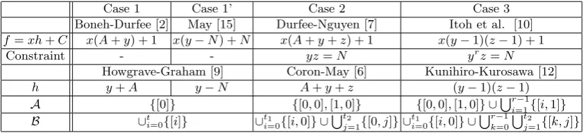
We show several examples of GSIP and argue applications of our compiler to them. Table 1 summarizes some example of GSIP in the literature. “Constraint” shows what kind of constraint variables have in both of solvingf = 0 andh= 0. “A” and “B” show what kind of generators we use in both of solving f = 0 and h= 0.
We give more explanation for each cases and give details of Case 1. More examples are given in Appendix B.
Case 1 Consider the small secret exponent attack on RSA by Boneh and Durfee [2]. In their attack, they handled f(x, y) = x(y +A) + 1 = 0 (mod e). Hence, this problem corresponds to h(y) = y +A
and C = 1. By using our compiler, the lattice basis for f(x) = 0 is automatically obtained. Then, one can easily obtain the bound:
Table 1.Examples of GSIP
Case 1 Case 1’ Case 2 Case 3
Boneh-Durfee [2] May [15] Durfee-Nguyen [7] Itoh et al. [10]
f=xh+C x(A+y) + 1 x(y−N) +N x(A+y+z) + 1 x(y−1)(z−1) + 1
Constraint - - yz=N yrz=N
Howgrave-Graham [9] Coron-May [6] Kunihiro-Kurosawa [12]
h y+A y−N A+y+z (y−1)(z−1)
A {[0]} {[0,0],[1,0]} {[0,0],[1,0]} ∪∪ri=1−1{[i,1]}
B ∪t
i=0{[i]} ∪ t1
i=0{[i,0]} ∪
∪t2
j=1{[0, j]} ∪ t1
i=0{[i,0]} ∪
∪r−1 k=0
∪t2
j=1{[k, j]}
Case 1’ Consider the small CRT exponent attack on unbalanced RSA by May [15]. In his attack, he handled f(x, y) = x(y −N) +N = 0 (mod e). Hence, this problem corresponds to h(y) = y −N and
C = N. By using our compiler, the lattice basis for f(x) = 0 is automatically obtained. Furthermore, one can easily obtain the bound
dp ≤e1−2(
√
β2+3β+β)/3
, whereq < eβ.
Case 2 Consider cryptanalysis on some variants of RSA with small se-cret exponent by Durfee-Nguyen [7]. In their attack, they handled the trivariate modular equation:f(x, y, z) =x(A+y+z) + 1 = 0 ( mod e) with constraintyz =N. Hence, this problem corresponds toh(y, z) =
A+y +z and C = 1. By using our compiler, the lattice basis for Durfee-Nguyen’s attack is automatically obtained.
Case 3 Consider the small secret exponent attacks on Takagi’s variant of RSA [19] by Itoh et al. [10]. This attack can be obtained by our com-piler and a lattice basis used in proving a deterministic polynomial equivalence between factoring and computing the secret exponent in that scheme [12]. Note that since Durfee-Nguyen technique is ade-quately involved in a lattice basis forh, we can easily obtain that for
f. One can easily obtain the bound: d < N(7−2√7)/3(r+1).
5.1 Case 1: Transforming Howgrave-Graham’s Lattice Basis to Boneh-Durfee’s Lattice Basis
Howgrave-Graham [9] provided an algorithm2 for solvingh(y) =A+
y = 0 (mod S) for integers A and S, which is an unknown divisor of an known integer U. Set shift-polynomials as h([j,ku)](y) := h[j,k]Nu−k =
yjh(y)kNu−k. In his paper, he chose the set of the indexes of shift-polynomials asH(u)=∪ku=0−1{[0, k]}∪∪ti=0{[i, u]}. We set a polynomial
or-der by this. Note that a generator is given byA={[0]}andB=∪ti=0{[i]}. Hence,H(u) holds Restrictions 1–3.
Letf(x, y) =x(A+y) + 1. We argue a lattice basis construction for
f. Sincef(x, y) =xh(y) + 1, we can employ our Compiler to construct a lattice basis forf. For a positive integerm, we define shift-polynomials for
f as f[i,j,k](x, y) = xiyjf(x, y)kMm−k. By our Compiler and Howgrave-Graham’s lattice basis, we have a set F as
F =
m
∪
u=0 {u−1
∪
k=0
{[u−k,0, k]} ∪
t
∪
i=0
{[0, i, u]} }
for fixed t. We have explicitly
F={[0,0,0],[0,1,0], . . . ,[0, t,0],[1,0,0],[0,0,1],[0,1,1], . . . ,[0, t,1],
[m,0,0],[m−1,0,1], . . . ,[0,0, m],[0,1, m],[0,2, m], . . . ,[0, t, m]}.
As you can easily verify, Boneh-Durfee’s set of shift-polynomials [2] and ours are completely the same as a set (but, a polynomial order is different). Then, they are the same as a lattice basis. So, we obtain the same lat-tice with Boneh-Durfee’s by using our compiler and Howgrave-Graham’s lattice basis [9].
Next, according to the discussion in Section 4, we will re-derive the bound of the secret key d. In [6], γU and γY are given as γU(u;t) =
u(u+ 1)/2 andγY(u;t) = (u+t)(u+t+ 1)/2. And, the dimension is given
byw(u;t) =u+t+ 1 andAY = logeY = 1/2. In this case, we can obtain
the same bound very easily. Since deg(γU(u;t)) = deg(γY(u;t)) = 2 and
deg(w(u;t)) = 1, Restriction 4 holds. Then, we can use Theorem 2. By ignoring small terms, we have a0 = 1/4, a1 = 1/2, a2 = 3/4, b1 =b2 = 1. By plugging these values into Eq. (8), one can easily obtain the bound
X < e1−4
√
4·1−3·1·2+3·1·3−8·1+3·2
3·4 =e(7−2
√
7)/6≈N0.284,
which is exactly same as the Boneh-Durfee’s weaker bound.
2
By employing his algorithm, Coron and May gave the deterministic polynomial time algorithm for factoring the RSA modulus under the condition that the secret keyd
5.2 Case 1’
By using the same lattice basis as Case1, we re-derive the small CRT-exponent attack [15]. By just replacingAY =β, we can derive the
condi-tion:dp < e1−2(
√
β2+3β+β)/3
, whereq < eβ.
6 Concluding Remarks and Open Problems
We note that our conversion is not enough. As shown in Sec. 5.1, our approach just achieves the Boneh-Durfee’s weaker bound. We need more analysis to achieve the stronger bound:d≤N0.292. Actually, Boneh and Durfee [2] deleted some badlattice bases and introduced the concept Ge-ometrically Progressive Matrix to evaluate the upper bound of the deter-minant of the lattice. By these efforts, they achieved the stronger bound
d ≤N0.292. We need to develop a general theory including such an im-provement.
Acknowledgement
The author thanks Kaoru Kurosawa for helpful discussions.
References
1. J. Bl¨omer and A. May, “A Tool Kit for Finding Small Roots of Bivariate Poly-nomials over the Integers,” in Proc. of Eurocrypt2005, LNCS 3494, pp. 251–267, 2005.
2. D.Boneh and G.Durfee, “Cryptanalysis of RSA with private key d less than
N0.292,” IEEE Transactions on Information Theory 46(4): 1339 (2000). (Firstly appeared in Eurocrypt’99).
3. D. Coppersmith, “Finding a Small Root of a Univariate Modular Equation,”in Proc. of Eurocrypt’96, LNCS 1070, pp. 155–165, 1996.
4. D. Coppersmith, “Finding a Small Root of a Bivariate Integer Equation; Factoring with High Bits Known,” in Proc. of Eurocrypt’96, LNCS 1070, pp. 178–189, 1996. 5. D. Coppersmith, “Small Solutions to Polynomial Equations, and Low Exponent
RSA Vulnerabilities,” J. Cryptology 10(4): 233-260, 1997.
6. J.S. Coron and A.May, “Deterministic Polynomial Time Equivalence of Computing the RSA Secret Key and Factoring,” Journal of Cryptology, Vol. 20, No. 1, pp. 39–50, 2007. (IACR ePrint Archive: Report 2004/208, 2004.)
7. G. Durfee and P. Nguyen, “Cryptanalysis of the RSA Schemes with Short Secret Exponent from Asiacrypt’99,” in Proc. of Asiacrypt2000, LNCS 1976, pp. 14–29, 2000.
8. N. Howgrave-Graham, “Finding Small Roots of Univariate Modular Equations Revisited,” IMA Int. Conf., pp.131–142 (1997)
10. K. Itoh, N. Kunihiro and K. Kurosawa, “Small Secret Key Attack on a Variant of RSA (due to Takagi),” In Proc. of CT-RSA2008, LNCS4964, pp. 387–406, 2008. 11. E. Jochemsz and A. May, “A Strategy for Finding Roots of Multivariate
Polynomi-als with New Applications in Attacking RSA Variants,” In Proc. of Asiacrypt2006, LNCS4284, pp. 267–282, 2006.
12. N. Kunihiro and K. Kurosawa, “Deterministic Polynomial Time Equivalence be-tween Factoring and Key-Recovery Attack on Takagi’s RSA,” In Proc. of PKC2007, LNCS4450, pp. 412-425, 2007.
13. N. Kunihiro, “Solving Generalized Small Inverse Problems,” to appear in Proc. of ACISP2010.
14. A.K. Lenstra, H.W. Lenstra, L. Lov´asz, “Factoring polynomials with rational co-efficients,” Mathematische Annalen 261, pp.515–534, 1982.
15. A. May, “Cryptanalysis of Unbalanced RSA with Small CRT-Exponent,” in Proc. of Crypto2002, LNCS 2442, pp. 242–256, 2002.
16. A. May, “Computing the RSA Secret Key Is Deterministic Polynomial Time Equiv-alent to Factoring,” in Proc. of Crypto2004, LNCS 3152, pp. 213–219, 2004. 17. A. May, Chapter3.2 “The univariate case,” in “New RSA Vulnerabilities Using
Lattice Reduction Methods,” Ph.D thesis, University of Paderborn, 2003. 18. R. Rivest, A. Shamir and L. Adleman, “A Method for Obtaining Digital Signatures
and Public-Key Cryptosystems,” Communications of the ACM, vol. 21(2), pp. 120–126, 1978.
19. T. Takagi, “Fast RSA-Type Cryptosystem Modulo pkq, ” in Proc. of Crypto’98, LNCS 1462, pp.318–326, 1998.
20. M. Wiener, “Cryptanalysis of Short RSA Secret Exponents,” IEEE Transactions on Information Theory, Vol. 36, pp. 553–558, 1990.
A Proofs
A.1 Proof of Lemma 4
The determinant of the submatrix Bu is given by
detBu =M(m−u)wX0uwdetB (u)
h (M) =M mw
(
X0
M
)uw
detBh(u)(M).
Since the determinant detB for f is given by detB = ∏mu=0detBu, we
have the lemma. ⊓⊔
A.2 Proof of Lemma 5
For Lemma 1, if the norm of bn+1 is less than Mm/ √
w, we can reduce the modular equations into integer equations. Combining Proposition 1, this condition can be transformed into
where γ is a constant. Since this term is negligible compared to MmW, we can ignore this term. By substituting Eq. (4) into Eq. (9), we have
(X0/M) ∑
uw(u)<
m
∏
u=0
(detBh(u)(M))−1. (10)
It is important thatMmW in both hand sides are canceled. By
transform-ing this inequality, we have the above condition. ⊓⊔
A.3 Proof of Theorem 2
The function l(m;t) is given by
l(m;t) = a0mt 2+a
1m2t/2 +a2m3/3
b1m2t/2 +b2m3/3
. (11)
By replacing x=t/m, we have
l(x)≡l(m;mx) = 6a0x 2+ 3a
1x+ 2a2 3b1x+ 2b2
.
The valuexminimizingl(x) satisfies 3a0b1x2+ 4a0b2x+ (a1b2−a2b1) = 0. If a1b2−a2b1 <0, this equation has a positive solution. By solving the above equation, we have
x= √
4a20b22−3a0a1b1b2+ 3a0a2b21−2a0b2
3a0b1
.
Letting this value c′ and plugging c′ into Eq. (7), we have the following condition for X0:
logMX0 <1− 4a0
b1
c′−a1 b1
.
In particular, if b1=b2, we have simply
c′ = √
4a20−3a0a1+ 3a0a2
3a0 −
2 3.
B More Examples
B.1 Application to Coron-May’s Lattice Basis to Durfee-Nguyen’s Lattice basis
Coron and May gave the deterministic polynomial time algorithm for factoring theunbalancedRSA modulus under the condition that the secret key d is given [6]. In the proof, they provided an algorithm for solving
h(y, z) = A+y +z = 0 (mod S) for integers A and S, which is an unknown divisor of an known integerU. Note thaty andz have relation:
yz =N.
Set shift-polynomials ash([j,k,lu) ](y, z) :=h[j,k,l]Nu−l =yjzkh(y, z)lNu−l. In their paper, they chose the set of the indexes of shift-polynomials as
H(u) =
u∪−1
k=0
{[0,0, k]∪[1,0, k]} ∪
t1
∪
i1=0
{[i1,0, u]} ∪
t2
∪
i2=0
{[0, i2, u]}.
Note that a generator is given by
A={[0,0],[1,0]}and B=∪t1
i1=0{[i1,0]} ∪
t2
∪
i2=1
{[0, i2]}.
Hence,H(u) holds Restrictions 1–3.
Letf(x, y, z) =x(A+y+z)+1 with constraintyz =N. We argue a lat-tice basis construction forf. Sincef(x, y, z) =xh(y, z)+1, we can employ our Compiler to construct a lattice basis for f. For a positive integerm, we define shift-polynomials forf asf[i,j,k,l](x, y) :=xiyjzlf(x, y, z)lMm−l. By our Compiler and Coron-May’s lattice basis, we have a setF as
F =
m
∪
u=0
u∪−1
k=0
{[u−k,0,0, k]∪[u−k,1,0, k]} ∪
t1
∪
i1=0
{[0, i1,0, u]} ∪
t2
∪
i2=0
{[0,0, i2, u]}
for fixedt1 andt2. As you can easily verify, Durfee-Nguyen’s set of shift-polynomials [7] and ours are completely the same as a set. Then, they are the same as a lattice basis. So, we obtain the same lattice with Boneh-Durfee’s by using our compiler and Coron-May’s lattice basis [6].
B.2 Application to Kunihiro-Kurosawa’s Lattice Basis to Itoh et al.’s Lattice basis
In this subsection, we simply writex, y, z, X, Y, Zinstead ofx0, x1, x2, X0, X1 and X2.
for an integerS, which is an unknown divisor of an known integerU. Note that y andz have relation: yrz=N.
Set shift-polynomials ash([j,k,lu) ](y, z) :=h[j,k,l]Nu−l =yjzkh(y, z)lNu−l. In their paper, they chose the set of the indexes of shift-polynomials as
H(u)=
u∪−1
k=0 {
[0,0, k]∪[1,0, k]∪
r∪−1
i=1
{[i,1, k]} }
∪
t1
∪
i1=0
{[i1,0, u]} ∪
r∪−1
i3=0
t2
∪
i2=1
{[i3, i2, u]}.
Note that a generator is given by
A={[0,0],[1,0]} ∪
r∪−1
i=1
{[i,1]} andB=∪t1
i1=0{[i1,0]} ∪
r∪−1
i3=0
t2
∪
i2=1
{[i3, i2]}.
Hence,H(u) holds Restrictions 1–3.
Let f(x, y, z) = x(y−1)(z−1) + 1 with constraint yrz = N. We
argue a lattice basis construction for f. Since f(x, y, z) = xh(y, z) + 1, we can employ our Compiler to construct a lattice basis for f. For a positive integer m, we define shift-polynomials for f as f[i,j,k,l](x, y) :=
xiyjzlf(x, y, z)lMm−l. By our Compiler and Kunihiro-Kurosawa’s lattice
basis, we have a set F as
F(u)=
u∪−1
k=0 {
[u−k,0,0, k]∪[u−k,1,0, k]∪
r∪−1
i=1
{[u−k, i,1, k]} }
∪
t1
∪
i1=0
{[0, i1,0, u]} ∪
r∪−1
i3=0
t2
∪
i2=1
{[0, i3, i2, u]}.
and
F =
m
∪
u=0 F(u)
B.3 Analysis for Non-linear h(y)
May [17] extended the Howgrave-Graham’s result [9] to analyze the case for univariate polynomial with higher-degree. By using May’s lattice basis, we analyze the case for the equation f(x, y) =xh(y) +C= 0 (mod M), where h is a univariate monic polynomial with degree κ ≥ 1 and C
is a non-zero integer. May [17] gave the set of indexes in the explicit form. A generator for h is given by A = ∪κi=0−1{[i]} and B = ∪ti=1{[i]}. The determinant of B(hu) by detB(hu)=Nκu(u+1)/2Yw(w−1)/2, wherew=
κu+t. By the similar analysis in Section 4, we have
X < M1−2
√
(βκ)2+3βκ−βκ
3 ,