THE DEVELOPMENT OF DEFORMABLE BODIES COLLISION RESPONSE ALGORITHM FOR INTERACTIVE VIRTUAL ENVIRONMENT
(PEMBANGUNAN TINDAK BALAS PELANGGARAN OBJEK BOLEH CANGGA UNTUK PERSEKITARAN MAYA INTERAKTIF)
NORHAIDA MOHD SUAIB ABDULLAH BADE
DAUT DAMAN
MOHD SHAHRIZAL SUNAR
PUSAT PENGURUSAN PENYELIDIKAN UNIVERSITI TEKNOLOGI MALAYSIA
ACKNOWLEDGEMENT
The researchers would like to express sincere gratitude to all parties and individuals involved, whether directly and indirectly in making this project a success, especially to the Ministry of Science, Technology and Innovation for providing funding for this research, Universiti Teknologi Malaysia (UTM) particularly the Research Management Centre, Faculty of Computer Science and Information System, fellow researchers and colleagues at the Department of Computer Graphics & Multimedia and all students involved. We are truly grateful for your support throughout this research.
ABSTRAK
Kaedah percanggahan berasaskan fizik lazimnya menghadapi masalah kerana memerlukan kos pemprosesan yang tinggi menyebabkan kaedah tersebut tidak sesuai untuk digunakan secara praktikal di dalam aplikasi interaktif, walaupun jika
percanggahan hanya berlaku pada kawasan kecik objek boleh canggah. Tesis ini mencadangkan kaedah percanggahan berasaskan pemilihan dinamik untuk objek yang mengalami percanggahan pada kawasan kecil. Ia dilakukan untuk memastikan
interaktiviti dengan objek berisipadu yang mempunyai bilangan geometri yang banyak dengan mengurangkan kawasan yang akan diproses untuk percanggahan. Kaedah ini adalah satu bentuk algoritma pengoptimum yang akan memilih kawasan yang akan diproses untuk percanggahan berdasarkan keadaan kestabilan kawasan tersebut. Dengan menganggap tiada tenaga lain yang bertindak ke atas objek boleh canggah selain
ABSTRACT
Physical based deformation method usually suffers from high computation cost which does not favors practical interactive applications, even if the deformation only occurs in a small area of the deformable object. This thesis proposed a dynamic selection based method for small area deformation to maintain interactivity with high geometric complexity of volumetric mesh by reducing areas for deformation processing. It is an optimization algorithm that selects small areas for deformation processing based on equilibrium state. Assuming no external forces other than concentrated loads, the
optimization algorithm succeeded to reduce deformation computation for physical based deformation systems. The method is suitable for real time application like virtual
TABLE OF CONTENTS
CHAPTER TITLE PAGE
TITLE i
DECLARATION ii
DEDICATION iii
ACKNOWLEDGEMENT iv
ABSTRAK v
ABSTRACT vi
TABLE OF CONTENTS vii
LIST OF TABLES xii
LIST OF FIGURES xiii
LIST OF APPENDICES xix
CHAPTER ONE INTRODUCTION
CHAPTER I INTRODUCTION
1.1 Introduction 1.2 Background 1.3 Problem statement
1 3
1.4 Objectives 1.5 Scopes
1.6 Dynamic selection based method 1.7 Results
1.8 Summary of chapters
8 8 9 10 11 CHAPTER TWO LITERATURE REVIEW
CHAPTER II LITERATURE REVIEW
2.1 Overview 2.2 Introduction
2.3 Deformable objects modeling 2.3.1 Input data
2.3.2 Data complexity 2.3.3 Accuracy
2.3.4 Interactivity 2.3.5 Flexibility
2.4 Non physical based modeling 2.4.1 Global deformation
2.4.2 Parametric representation 2.4.3 Free form deformation 2.4.4 Pros and Cons
2.5 Physical based modeling 2.5.1 Finite element method 2.5.2 Mass spring method 2.5.3 Gas pressure method 2.5.4 Mesh free method
2.5.5 Pros and Cons
2.6 Real time modeling technique
58 58
CHAPTER THREE METHODOLOGY
CHAPTER III METHODOLOGY
3.1 Project planning 3.2 Theoretical framework 3.3 Software development 3.4 Testing methodologies 3.5 Software specifications 3.6 Hardware specifications
67 67
70 74 74 75
CHAPTER FOUR IMPLEMENTATION
CHAPTER IV IMPLEMENTATION
4.1 Introduction 4.2 Preparing data
4.3 Building the framework 4.4 Performance issues 4.5 General strategy
4.6 Building algorithm template 4.7 Defining non-equilibrium state
76 76
4.8 Relative distance from node to its neighbor as equilibrium state 4.9 Distance from current node
position to previous node position as equilibrium state 4.10 Node’s linear velocity as
equilibrium state 4.11 Algorithm 4.12 Data structure 4.13 Conclusion
87 89 91 94 95 96 CHAPTER FIVE ANALYSIS
CHAPTER V ANALYSIS
5.1 Introduction
5.2 Evaluation of algorithms 5.3 Results and benchmarks 5.3.1 Goals
5.3.2 Benchmarking method 5.3.3 Specifications
5.3.4 Input data
5.3.5 Benchmarks against other method
5.3.6 Benchmarks against various settings
5.4 Other issues 5.5 Conclusions
CHAPTER SIX CONCLUSIONS
CHAPTER VI CONCLUSIONS
6.1 Introductions 6.2 Summary 6.3 Contributions 6.4 Future work
121 121
LIST OF TABLES
NO. TITLE PAGE
2.1 Values for the Young’s modulus of multiple solid materials. (Cutnell and Johnson, 1995)
20
4.1 The cost for activation and deactivation test for best case scenario (1 node and 3 neighbors).
89
4.2 The cost for activation and deactivation test for best case scenario (1 node and 3 neighbors).
90
4.3 The cost for activation and deactivation test for best case scenario (1 node and 3 neighbors).
92
5.1 The cost of activation and deactivation test comparison for best case scenario (1 node and 3 neighbors).
99
5.2 Details of input data. 103
LIST OF FIGURES
NO. TITLE PAGE
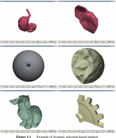
1.1 Example of dynamic selection based method. 9 2.1 Taxonomy of deformable objects for this thesis. 14 2.2 Catheter Angiography : X-ray equipment is mounted on a C-shaped
gantry with the x-ray tube itself beneath the table on which the patient lies. Above the patient is an image intensifier that receives the x-ray signals, amplifies them, and sends them to a TV monitor.
(http://www.radiologyinfo.org/content/diagnostic/diagnostic.htm)
16
2.3 CTA scan equipment.
(http://www.radiologyinfo.org/content/diagnostic/diagnostic.htm)
17
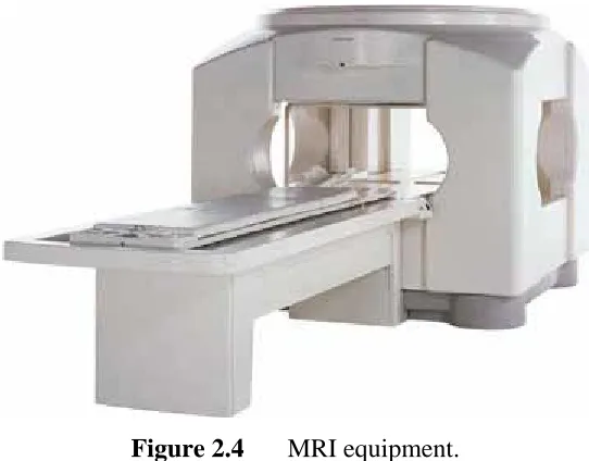
2.4 MRI equipment.
(http://www.radiologyinfo.org/content/diagnostic/diagnostic.htm)
17
2.5 Ultrasound (sonography) equipment.
(http://www.radiologyinfo.org/content/diagnostic/diagnostic.htm)
18
2.6 Voxelman showing registration of several data sources.
(http://biocomp.stanford.edu/3dreconstruction/software/voxelman.html)
18
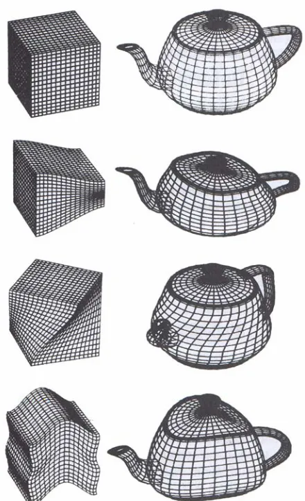
2.7 Stress strain graph indicates elastic and plastic (inelastic) deformations. 19 2.8 Stress strain graph showing multiple type of relation for deformations. 20 2.9 Structures deforming global deformation example. Top, original cube
and Utah teapot followed by tapering, twisting and bending deformations. (Watt and Watt, 1992)
26
2.10 Example of NURBS surface 27
(Sederberg et al., 1986)
2.12 Extended free form deformations (Coquilart, 1990). Top left, a sphere deformed with a parallelepiped lattices. Top right, a sphere deformed with a cylindrical lattice. Middle left and right, deformed lattice and the deformed surface. Bottom left and right, resulting sand pie.
29
2.13 Hirota’s volume preserving method. Letf, original shape. Center, after free form deformation is applied. Right, unconstrained lattices are displaced to preserve original volume(Hirota et al, 1999)
31
2.14 Deformable teapot is animated using dynamic global free form deformation. ( Faloutsos et al., 1997)
32
2.15 Three type of geometry discretization using gmesh (Geuzaine and Remacle, 2005).
37
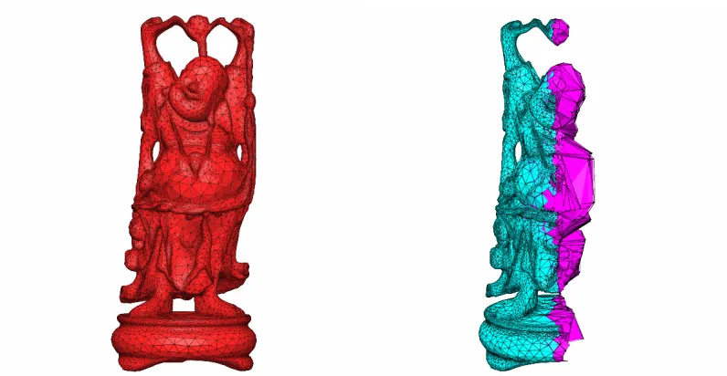
2.16 Original happy buddha and its sliced tetraheralized version. Happy buddha is discretized using tetgen application(Si, 2005)
37
2.17 Taxonomy for finite element method from mechanical physics view. (http://caswww.colorado.edu/courses.d/AFEM.d/Home.html)
38
2.18 Top,the three standard solid element geometries: tetrahedron (left), wedge (center) and brick (right). Only elements with corner nodes are shown. Middle, regular 3D meshes can be built with cube-like
repeating mesh units. Meshes are built with bricks, wedges or
tetrahedra. Bottom, two nonstandard solid element geometries: pyramid and wrick (w(edge)+(b)rick). Four faces meet at corners 5 and 7,
leading to a singular metric.
(http://caswww.colorado.edu/courses.d/AFEM.d/Home.html)
39
2.19 A simple finite element method deformable object in action. Image is taken from project Xplodar
(http://nesnausk.org/nearaz/projXplodar.html). High contrast red denotes high stress area while bright white denotes less stress area. Even though the simulation is performed in real time manner, notice that the deformable object is low in polygons.
41
neighboring points, displacing the points from its rest position. (Gibson and Mirtich, 1997)
2.21 Example of gaseous pressure method for simple two dimensional meshes. The mesh must be manifold, represented as wrapped cloth which will have ideal gas pressure inside. (Matyka and Ollila, 2003)
49
2.22 Screen shot of of gas pressure method for three dimensional volumetric deformable objects (Matyka and Ollila, 2003). The simulation is fast enough to be performed in real time.
50
2.23 Rendering techniques for particle based surface; axes, discs, wireframe triangularion and flat shaded triangulation (Tonnesen and Szeliski, 1992)
53
2.24 Left, deforming. Center, deforming and surface restructuring by adding new points. Right, deforming and tearing. (Tonnesen and Szeliski, 1992)
53
2.25 Fusioning deformable objects (Tonnesen and Szeliski, 1992) 54 2.26 Deformable object are splitted and then fused together. (Desbrun and
Cani, 1996)
55
2.27 Target morph using point based method. (Keiser et al., 2004) 56 2.28 Debunne et al. uses local refinement of multiresolution models to
reduce computation time by reducing geometry for run time dynamics processing. (Debunne et al., 2001)
60
2.29 Dynamic progressive meshes is used to refine local contact area to enhance dynamics computation (Wu et al., 2001)
61
2.30 Vertices of the surface mesh are displaced according to the displacement field of the tetrahedron in which they lay using barycentric coordinate system (Muller and Gross, 2004).
58
2.31 Chen et al. mass spring systems lattice configurations adapted from Provot cloth mass spring configurations (Chen et al., 1998).
63
2.32 A low resolution tetrahedral mesh and a high resolution surface mesh of a snake. Deformation is computed for low resolution tetrahedral mesh using mass spring systems and high resolution mesh is used for
rendering.(Teschner et al, 2004).
2.33 Chainmail works by constraining distances between neighboring points (Gibson 1997). Upper left image shows initial state of the chainmail systems. Upper right image shows deformed chainmail systems. Lower left image shows chainmail systems at its initial state. Lower middle image shows maximally compress chainmail and lower right shows maximally stretch chainmail.
65
3.1 Conceptual diagram of the deformable object systems. 68 4.1 Stereolithography file format requirements. 1. No open edge. 2. No
double face. 3. No spike. 4. No multiple edges. (Images from 3D Studio Max 7.0 Reference Manual)
77
4.2 Example of tetrahedral with no quality enforcement. (Images from Tetgen 1.3 Manual)
78
4.3 Example of tetrahedral with quality enforcement. (Images from Tetgen 1.3 Manual)
78
4.4 Some example of tetrahedral meshes viewed with Tetgen viewer. In top-left to top right order, the data are Stanford bunny, Stanford bunny internals, human stomach, human stomach internals, sphere and human liver. All of them are freely available on the internet except for sphere which is generated using discreet 3D Studio Max 7.0. Screenshots were taken using Tetgen Viewer.
80
4.5 Conceptual flow of common physical simulation after inserting optimization algorithm.
81
4.6 Example of activation systems in 2d. (1) Concentrated loads are applied to a node. (2) When the node reaches its non-equilibrium state, it will activate its neighbor. (3) The activation process continues until the node reaches its equilibrium state. Inactive nodes will act as constraint. Active nodes reaching equilibrium state will be deactivated.
84
4.7 Activation test. If (|sr(t1)-sn(t1)| > dcache*threshold || |sr(t1)-sn(t1)| <
dcache*threshold), activates its neighbor, sn(t1). In other words, if current
distance, dcurrent is more than dcache multiplied with threshold or current
distance, dcurrent is less than dcache multiplied with threshold, activate the neighbor, sn.
4.8 Deactivation test. If (|sr(t1)-sr(t0)| > threshold), deactivate itself, sr. In other words, if current distance, dcurrent is less than threshold, deactivate the actor sr.
88
4.9 Activation test. If (|sr(t1)-sr(t0)| > threshold). In other words, if current
distance, dcurrent is greater than threshold, activate all neighbors.
Deactivation test is exactly the same from previous method (see Figure 4.8).
90
4.10 Inconsistencies of using simple magnitude measuring by using per axis test. v1 and v2 are linear velocities with the same magnitude, tx and ty are axis threshold and x and y are axis. v2 passed the non equilibrium test while v1 failed the non equilibrium test even when both share the same magnitude.
92
4.11 Activation test. If (|sv(t1)| > threshold), activate all its neighbors. In other
words, if current node velocity, sv(t1) is greater than threshold, activate
all its neighbors.
92
4.12 Deactivation test. If (|sv(t1)| < threshold), deactivate itself, sr. In other words, if current node velocity, sv(t1) is lesser than threshold, deactivate
itself, sr.
92
4.13 Example deformations of Stanford bunny data.(Top left image is the undeform pose)
96
5.1 The statistic comparison of benchmark input data. 102 5.2 Input data for benchmark are bunny100 (top left), bunny500 (top right),
bunny1000 (bottom left) and icosa12 (bottom right).
103
5.3 Benchmark charts for bunny100. 106
5.4 Benchmark charts for bunny500. 108
5.5 Benchmark charts for bunny1000. 109
5.9 Total active nodes benchmark result for icosa12. 115 5.10 The higher the number of active nodes, the lower the performance for
simulation systems with optimization algorithm.
117
5.11 The optimal threshold must suited for the node to be displaced to the imaginary position which is the position where the node will be render at adjacent pixel.
118
5.12 When node and its neighbor occupy the same pixel in the viewing device, the optimal threshold must suit for the smallest distance from node to neighbor between all neighbors.
LIST OF APPENDICES
CHAPTER I
INTRODUCTION
This chapter describes the context of the work, presents the research statement, and provides an overview of the report.
1.1 Introduction
Achieving interactive deformation is a crucial part in computer animation and medical applications. Deformable modeling can assist artist in modeling 3D content for computer animation by enabling higher degree of controls for modeling tools. These tools reduce artist workload and provide better results in less time compared to traditional method without deformation tools. Another form of deformation
modeling, physical based deformation, used by computer animation to provide a method to simulate the behaviour of real world materials. The results are visually convincing in terms of realistic depiction of the real world compared to traditional animation method. With physical based animation, artists are no longer required to manually key framed the animation as the task has been shifted to the physical based animation system.
Deformation modeling also has found its way to medical field. It is used mainly to simulate the behavior of soft tissues of the human body. One example of medical application is virtual surgery which allows trainee surgeons to feel and see exactly what they would if they were operating on real patient. This may help improve surgical skills of the surgeons as it would with pilot trained in flight simulator. The use of virtual objects reduces the cost of obtaining real material for surgical training and reduces the offensive nature of using real dead bodies for training. With virtual surgery application, surgeons can plan ahead the surgical procedures and perform surgical test without the risk of failure. However, the
complex nature of the human tissue and the demanding accuracy required by medical application makes it a very challenging domain.
The field of deformable object modeling has seen many improvements throughout the years. This will be discussed in Section 1.2 (background and previous works that are related to this research). This is followed by the problem statement in Section 1.3, Section 1.4 lists the research objectives, Section 1.5
1.2 Background
Computer graphics modeling had only been for rigid objects until Barr introduced global deformation technique, more than two decades ago (Barr. 1984). The idea behind this method is to apply another transformation to existing
transformation before transformation is applied to the objects. In order to allow more deformation control over the objects, Sederberg introduced free form deformation (Sederberg et al. 1986). The method models non solid object behaviour by changing the object according to the changes experience by enclosing lattices. Both methods have been used extensively in 3D modelling tools and CAD tools. However, both deformation methods lack one crucial feature, and that is physical behaviour.
In order to allow physical behaviour to the deformable object, Terzopoulos proposed an elastic physical based deformation method in 1987 for use in pre-computed computer generated animations (Terzopoulos et al. 1987). Later, he introduces inelastic physical behaviour such as viscoelasticity, plastic and fracture (Terzopoulos and Fleischer, 1988). Then in 1989, he presents a method to model the behaviour of fluid like molten objects (Terzopoulos et al. 1989). Generally,
Terzopoulos and his colleagues proposed methods that are based on simplification of elasticity theory to model various physical behaviours for use in pre-computed computer generated animations.
The behaviour of deforming objects is the topic of continuum mechanics, a branch of mathematics that tries to capture physical phenomena of continuous media in precise mathematical formulations. One branch of continuum mechanics,
deformation behaviour. However, due to the nature of the system and the complexity of the method, the method cannot be applied directly to real time animation systems.
Thus, Bro-Nielsen proposed a fast finite element method for use in virtual surgery environment (Neilson and Cotin, 1996). He uses condensation techniques to reduce the complexity of the system equations and thereby achieve a considerable speed-up compared to the volumetric models in (Cotin et al. 1996). The effect of using condensation techniques is low generality of the simulations, i.e. no rapid displacement, no great displacement. Based on the principle of superposition, Cotin proposed a higher generality deformation system (Cotin et al. 1999). Although the method experienced high frame rate, it was implemented on low resolution mesh. Furthermore, pre computation method used does not permit topological changes to the deformable objects.
By using high resolution mesh, the deformation behaviour can be modeled in higher accuracy. The problem with high resolution mesh is that it costs more
computational resources. To reduce computational resources, several researchers have opted to use multi-resolution method in the mesh domain. Debunne uses automatic space and time adaptive object representation level of detail technique to allow local refinement or simplification of the computation model based on local error measurement (Debunne et al. 2001). Krysl uses adaptive local finite element mesh refinement using wavelet theory to accelerate finite element deformation (Krysl et al. 2003). Although both methods produce acceptable frame rates on high resolution mesh, they still suffer from high computation required by finite element method.
2003). To model deformation for volumetric objects, the deformable object must first be discretized as one would with finite element method. The prominent problem of mass-spring systems is numerical instability under large time step (Baraff and Witkin, 1998). For large number of mass-spring nodes, the simulation system
quickly converges error and became unstable. One solution to the stability problem is Verlet integrator, which capable of maintaining stability even for large number of nodes (Jacobsen 2003). Unfortunately, for deformable object with extremely large number of nodes, mass spring system is still too slow to be used for interactive systems.
By using simple mathematical approach for deformation processing, Gibson proposed a fast deformation method for extremely large number of nodes (Gibson, 1997). The method known as ChainMail, perform deformation based on nodes distance constraint. However, due to the used of simple distance constraints for deformation instead of continuum-based physics, the resulting behaviors are not physically convincing. Plus, it is hard to define real world materials. Nevertheless, ChainMail contributed new approach in the field of deformable object modeling by introducing force propagation method. Force propagation method works like sound wave effect in the sense that areas near contact are first displaced and displacements are propagated throughout the object.
algorithm was tested for surface deformation only. Choi et al. used static selection of neighbouring nodes to handle deformation (Choi et al. 2002, Choi et al. 2003). One critical problem of the algorithm is that the deformation area cannot be scaled as needed. A special method is required to handle multiple contacts. Another improvement to the ChainMail algorithm is made by Park et al. who extended ChainMail algorithm by preserving original shape by keeping track of the direction vector from current node position to the original node position (Park et al. 2002).
This research tries to find solutions to the above mentioned problems noted by previous researchers.
1.3 Problem statement
The advent of hardware acceleration rendering support has made geometry a popular choice for real time and interactive applications rendering. With increasing complexity of 3D geometric data and growing demand for realistic deformation functionality, significant effort is being devoted to the design of robust, fast, and scalable algorithms for geometry deformation processing. The problem for
For small deformation based on concentrated loads, the largest primitive elements’ (vertices) displacements are on the area near applied concentrated loads. The further the elements distance from the contact point centre, the lesser force experienced by the elements. This is due to the damping forces conducted by every passing element during force propagation. Similar phenomena can be observed by softly touching a pillow. Notice that only small area near touched area are deformed. Traditional deformation methods perform deformation processing throughout the object even if the vertices did not experience noticeable deformation or if the vertices did not experience any deformation at all. Based on this observation, this research proposed a deformation method where deformation will be process on the areas that are most likely to experience noticeable deformation for non critical interactive applications. This way, the effect upon having high geometry deformable objects seems transparent for total application performance as the system only process deformation for a limited sets of elements.
This research addresses the deformation processing problem for small deformation situations. The hypothesis is stated as:
The cost of deformation processing can be reduced by only deforming small
1.4 Objectives
It is desirable to put computation resources where it will be most beneficial. To this effect, this research outlines the most critical objectives as follows:
1. To inquire into appropriate deformable objects representation.
2. To investigate, analyze and formulate an appropriate technique for collision response encompassing deformable objects adequate for interactive
application.
3. To develop an algorithm of collision response for deformable body motion. 4. To design and develop a real-time simulation model based on objects
representation and handling of real-time collision response.
1.5 Scopes
The scopes of this project are as follows:-
• Deformable volumetric objects are represented geometrically.
• Objects are manifold and do not experience topological changes such as
cutting and fracture.
• Deformations are performed based on concentrated loads.
• Object deformations are fully elastic. Deformed objects should return to its
original state after removal of applied external forces.
• Interactions are described as single manipulator tool versus deformable object
vertex.
• No volume preservation.
1.6 Dynamic selection-based method
This research proposed an algorithm known as dynamic selection-based method. In short, the algorithm reduces the cost of deformation processing by
dynamically select small areas for deformation. It is used with mass-spring system as the main deformation system.
Dynamic selection based method is highly inspired by force propagation theory. Known as ChainMail, it was first introduced for deformable modeling by Sarah F. Gibson (Gibson. 1997). Based on the reviews, ChainMail doesn’t seem to include any physical based justification in its deformation. In depth discussion of this topic are available in Chapter 4.
1.7 Results
The results from this research are summarized as follows:
Object representation: Deformable objects are represented using mass-spring model.
Reduced area for deformation: For every frame, deformable object is evaluated for deformation. The result from the evaluation is a small area of deformable object that will be selected for deformation. Similar in nature to
ChainMail (Gibson 1997), this will reduce required deformation processing time as only small areas are actually deformed per frame.
Dynamically enlarge or shrink deformation area: Unlike previous
deformation method inspired by force propagation, dynamic selection based method can dynamically enlarge or shrink deformation areas. Previous works usually either resort to static range of areas (Choi et al. 2003) or propagate over the deformable object infinitely (Dusyak and Zhang. 2004). Other methods that can dynamically enlarge or shrink deformation area do not have physical-based justifications in their deformations.
1.8 Summary of chapters
This section presents a brief overview of the content of this report.
Chapter II: An overview of previous works on deformation method, real-time performance strategy and force propagation-based method.
Chapter III: Implementation planning was outlined here. Acceleration strategies were described along with its justifications. Both hardware and software specification requirements are discussed here.
Chapter IV: Detail discussions on implementation starting from building the data, algorithm loops and algorithm.
Chapter V: Results and benchmarks of the research. It provides analytical performance results, discussion of various issues regarding the performance and quality of deformation behaviors of the proposed algorithm.
CHAPTER II
LITERATURE REVIEW
2.1 Overview
In this chapter, elementary theories and techniques that are relevant in volumetric object deformation are discussed. Presented next are literatures for both non-physical-based modeling and physical-based modeling of deformable objects. Then, the discussion will cover previous work on real-time acceleration techniques.
2.2 Introduction
most 3D animation package where cloth deformations are simulated for scene environment throughout animation time. Often considered as physical-based
deformations, the cloth tools tries to find the equilibrium state for the cloth based on interacting forces. For deformable objects editing, there will be a mechanism or method which facilitates the deformation of object deformations. For example, free form deformation tools available in most 3D animation packages where the objects are deformed to satisfy constraint that are manipulated by user. Often considered as non-physical based deformation, the free form deformation method will displace primitives (with specific constraints) until it reached a new position which satisfies the constraints.
Physical-based deformation for solid objects (non-liquid and non-gaseous matter), based on theory of elasticity, can be either be elastic or inelastic (plastic). Elastic objects are objects that return to their original states after removal of applied forces. Contrary to elastic objects, inelastic objects are objects that do not return to their original state after applied forces have been removed due to atomic plane dislocation in the real materials. Technically, all objects should be considered inelastic, due to the fact that every object can experience atomic plane dislocation. But due to performance reason, most objects that behave elastically during the simulation can be considered as elastic objects. Fundamental measurements of deformed object are by its dimension; length for one dimensional objects, surface area for two dimensional objects and volume/bulk for three dimensional objects. For three dimensional cases, deformable objects are represented with volumes that have both surface structure and internal structure. There are three types of forces;
concentrated loads, distributed loads over the body and distributed loads over the surface of on object. Concentrated loads are forces applied at discrete points. Example of concentrated loads is force exerted when a pencil tip is pressed onto a pillow. The second type of force is loads distributed over the body. Such is
Volumetric deformable objects can be represented by geometric mesh, iso-surface, voxels, points etc. Geometric mesh-based rendering can be accelerated efficiently by 3D hardware compared to other methods of rendering.
Figure 2.1 Taxonomy of deformable objects for this research.
2.3 Deformable objects modeling
application requirements, the application traded off less important simulation features to provide the desired features more computational power.
2.3.1 Input data
Since current 3D hardware has matured enough to support geometric
rendering, the focus of this research will be on techniques to acquire geometric data. Geometric data can be acquired by designing, 3D scanner, diagnostic radiology or from mathematical models. Modeling tools such as Autodesk® 3ds Max®, Autodesk® Maya®, NewTek Lightwave 3D®, Robert McNeel & Associates Rhinoceros®
NURBS modeling allow designers to create, edit and analyze vertices, lines, curves, planes, surfaces and solids to produce the desired objects. These data can be saved as geometry, mathematical parameters or boundary elements (constructive solid
geometry, boundary representations). To acquire data from real world object, one can use 3D scanners available from Cyberware, Northern Digital Inc. and Cognitens Ltd., to name a few. Data acquired using laser scanning, electromagnetic resonance or multiple sets of 2D images reconstruction, are highly accurate compared to artist impression of the objects. Diagnostic radiology enables one to get information of a particular object including both surface and its underlying structure. By analyzing reflection, penetration or emitted energy of transmitted light wave (x-ray),
electromagnetic wave, sound wave (ultrasound) or nuclear energy, underlying structure can be constructed without the need to cut the physical objects. These methods of data acquisition are very useful in medical applications as no significant harm done to the patient to get the underlying structure image. Some example of x-ray imaging equipment is computer tomography scan (CT scan), athrography and mammography. Hysterosonography use ultrasound waves to show structures in the human body. The sound waves reflect off internal organs and other anatomic structures to create images. Magnetic resonance imaging (MRI) is a method of producing extremely detailed pictures of body tissues and organs using
patient to radiofrequency waves in a strong magnetic field is measured and analyzed by a computer, which forms two- or three-dimensional images that may be viewed on a TV monitor. Nuclear medicine is a subspecialty within the field of radiology. It comprises diagnostic examinations that result in images of body anatomy and function. The images are developed based on the detection of energy emitted from a radioactive substance given to the patient, either intravenously or orally. Voxelman register together data from various sources (CT, MRI, X-ray) to create visualization of human skull anatomy. Data acquired using diagnostic radiology has to be
reconstructed as geometric data before performing geometric deformation.
Geometric data can also be generated by mathematical models using fractal, implicit method or by spline-based technique.
Figure 2.2 Catheter Angiography : X-ray equipment is mounted on a C-shaped gantry with the x-ray tube itself beneath the table on which the patient lies. Above the patient is an image intensifier that receives the x-ray signals, amplifies them, and
Figure 2.3 CTA scan equipment.
Figure 2.5 Ultrasound (sonography) equipment.
Figure 2.6 Voxelman showing registration of several data sources.
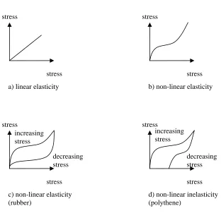
Breen, 2000) is a standard set of fabric measuring equipment that can measure the bending, shearing and tensile properties of cloth. The equipment measures force or moment that is required to deform a fabric sample of standard size and shape, and produces plots of force or moment as a function of measured geometric deformation. From physics literature (Yong and Nagappan, 2003) (Cutnell and Johnson, 1995), material properties can be divided into five phases; limit of proportionality, elastic limit, yield point, breaking stress and breaks (as illustrated in Figure 2.7).
stress
plastic deformation elastic deformation
A = limit of proportioanlity B = elastic limit
C = yield point D = breaking stress E = breaks
strain O
ABC D E
stress stress
stress stress
b) non-linear elasticity a) linear elasticity
stress stress
Figure 2.8 Stress strain graph showing multiple type of relation for deformations.
Table 2.1 Values for the Young’s modulus of multiple solid materials. (Cutnell and Johnson, 1995)
Material Young’s Modulus Y (N/m2) Aluminium 6.9 x 10¹⁰
Bone Compression 9.4 x 10⁹ Bone Tension 1.6 x 10¹⁰
Brass 9.0 x 10¹⁰
Brick 1.4 x 10¹⁰
Copper 1.1 x 10¹¹
Mohair 2.9 x 10⁹
Nylon 3.7 x 10⁹
Pyrex glass 6.2 x 10¹⁰
Steel 2.0 x 10¹¹
Teflon 3.7 x 10⁸
Tungsten 3.6 x 10¹¹
stress stress
increasing increasing
stress stress
decreasing decreasing
stress stress
c) non-linear elasticity (rubber)
2.3.2 Data complexity
Usually, in computer graphics term, complex polygonal object refers to object with large number of polygons. Since computers have limited total triangle fill rate per second, reducing the poly count is always a better choice, as long as the object maintains its original looks. For deformable object modeling, this is not
usually the case. Object with low poly counts can still slows the system down. This is due to the cost of deformation calculation for every primitive element of the objects, which is expensive. Different algorithm varies in its computation cost, but at the end, the bottleneck is usually the CPU processing power, not the GPU processing power. Thus, for deformable object, it is recommended to reduce the geometry of
deformable object representation as long as it can undergo deformation to the required extent with acceptable results.
Another thing to consider is mathematical complexity of the deformation process. To achieve accurate results, one has to resort to use accurate computation techniques usually originated from mechanical dynamics in physics. These accurate techniques are suitable for highly risky simulation such as virtual surgery. But, a large number of computation tends to prevent the simulation to be performed in interactive manner. Mathematical complexity can be reduced by using simpler ordinary differential equation solver (Teschner et al. 2004), assuming fixed state (Matyka, 2003), pre-compute complex computation (D. L. James and Fatahalian, 2003) etc..
Different deformation techniques vary in its object representation memory consumption. Complex object requires enough memory to store its large geometric structure including internal geometric structure and its material properties.
2.3.3 Accuracy
Required accuracy varies between different types of applications. Depending on the application requirements and involved risk, end results can either be
interactively manipulated, physically realistic or physically plausible. Deformation accuracy can be divided into three; geometric accuracy, mathematical accuracy and physical accuracy. To achieve high geometric accuracy, virtual object must closely resemble its real world counterpart. High mathematical accuracy can be achieved by using accurate computation technique. For example, there are multiple ordinary differential equation solvers, and most of them will accumulate precision error over time. Choosing the most precise technique will delay noticeable inaccuracies and maintain the system stability for a longer period of time. Simulating deformation true to the atom level is very expensive as even the smallest visible object contains large number of atoms. Even when the technologies are able to simulate deformation by displacing atoms, the visual difference is hardly noticeable and less required for mainstream applications. Approximating physical accuracy can be done in various ways such as neglecting small deformation factor, assuming the material is a
anisotropic or non-heterogenous material and assuming linear elasticity deformation.
2.3.4 Interactivity
In computer graphics modeling, it is essential to have deformation tools that are robust and fast enough to be used interactively. Simple deformation technique like global deformation (Barr, 1984) is very limited in its deformation ability compared to free form deformation (Sederberg and Parry, 1986). Unlike
the interactions are known and limited, deformation can be pre-computed to enable user interaction.
It is desirable to have user control (to some degree) over the deformable objects deformation motion instead of giving the dynamics formulation a total control. This is especially true for computer animation and cartoon animation as it can give animated characters unique behaviors.
2.3.5 Flexibility
Deformation robustness and flexibility are the ability of the deformation technique to support heterogeneous tissues, topological changes and material parameters changes. Human tissues consist of multi-layered, varied stiffness materials. Terzopoulos and Waters apply dynamic mass-spring system to facial modeling by constructing a three layer mass-spring mesh of dermal, fatty and muscle layer (Terzopoulos and Waters, 1990). Under certain conditions such as when
2.4 Non-physical based modeling
3D designers require precise deformation tools which give them total deformation control. These tools usually come as purely geometric modification tools which do not include any physical justifications in its deformation process. The output relies on the skill of the designer and how much control the deformation technique provides. Three most popular non-physical based modeling techniques are discussed as follows; global deformation, parametric representation and free form deformation.
2.4.1 Global deformation
In 1984, Barr introduced global deformation technique by extending the classical linear transformation operation (Barr. 1984). The idea behind this method is to apply another transformation to existing transformation before it is applied to the object. The available deformations are tapering, twisting and bending. Given a function for the transformations:
) ( ),
( ),
(x Y F y Z F z F
X = x = y = z ,
where (x, y, z) are vertices in undeformed state, and (X, Y, Z) is the deformed vertex.
Object is tapered by choosing a tapering axis and differentially scales the other two axis components, setting up a tapering function along tapering axis. For example of tapering an object along its z-axis, X =rx,Y =ry,Z = z, where
is the tapering function either linear or non-linear. To globally twist the
object, use differential rotation just as tapering is a differential scaling. To twist an object through an angle
) (z f r=
θ about the z-axis, we apply
) , cos sin , sin cos ( ) , ,
By varying the amount of rotation as a function of z, the object will become twisted. This is done by setting θ = f(z) where f(z) specifies the rate of twist per unit length
along the z-axis. To bend an object along y-axis, the deformation transformation is given by x X = ⎪ ⎩ ⎪ ⎨ ⎧ > − + + − − < − + + − − ≤ ≤ + − − = − − − max max 0 1 min min 0 1 max min 0 1 ) ( cos ) ( sin ) ( cos ) ( sin ) ( sin y y y y y k z y y y y y k z y y y y k z Y θ θ θ θ θ ⎪ ⎩ ⎪ ⎨ ⎧ > − + + − < − + + − ≤ ≤ + − = − − − − − − max max 1 1 min min 1 1 max min 1 1 ) ( sin ) ( cos ) ( sin ) ( cos ) ( cos y y y y k k z y y y y k k z y y y k k z Z θ θ θ θ θ
where is the bending region, is the radius of curvature of
the bend, the center of the bend is at
max
min y y
y ≤ ≤ k−1
0
y
y = , the bending angle is θ =k(y'−y0)and
⎪ ⎩ ⎪ ⎨ ⎧ ≥ < < ≤ = max max max min min min ' y y y y y y y y y y y
Baraff and Witkin (Baraff and Witkin, 1992), uses connected global deformation elements to create flexible object deformation systems.
Figure 2.9 Structures deforming global deformation example. Top, original cube and Utah teapot followed by tapering, twisting and bending deformations. (Watt and
Watt, 1992)
2.4.2 Parametric representation
Figure 2.10 Examples of NURBS surface.
Given a set of n + 1 control points the corresponding Bézier
curve (or Bernstein-Bézier curve) is given by
, ,..., , 1
0 P Pn
P
∑
= = n i n i iB tP t C 0 , ( ), ) (
where Bi,n(t) is a Bernstein polynomial and t∈[0,1]. These functions are scaled or
weighted by , the network of control vertices, to form the surface patch. A cubic
Bézier patch, an extension to the Bézier curve, is given by, i P
∑
∑
= = = 3 0 3 0 ) ( ) ( ) , ( j j i ij i v B u B P v u Q .A generalization of the Bézier curve is the B-spline curve. As an
improvement over the Bézier representation, B-spline are superior over the Bézier method within the context of deformation as B-Spline does not require continuity constraint and this gives the user the ability to perform localize deformation. Since the absence of continuity constraint, B-spline curve restricted the deformation by control points to only specific known region thus giving better control to the deformation made by the user.
2.4.3 Free form deformation
Figure 2.11 Right, local free form deformation. Left, global free form deformation. (Sederberg et al., 1986)
undergoes. The embedding space called FFD block, are actually hyperpatches connected together to form a piecewise Bézier volume.
Figure 2.12 Extended free form deformations (Coquilart, 1990). Top left, a sphere deformed with a parallelepiped lattices. Top right, a sphere deformed with a cylindrical lattice. Middle left and right, deformed lattice and the deformed surface.
Bottom left and right, resulting sand pie.
A single tricubic Bézier hyperpatch is defined as
where , and are the Bernstein polynomials of degree 3. The
undeformed FFD block consists of a rectangular lattices of control points arranged along three mutual perpendicular axes. The end result is a parallelepiped with lattices as control points attached. To deform an object using free form deformation method, we must first determine the positions of the vertices in the lattice space. Then deform the FFD block by displacing the control points from the undeform lattice positions. Finally, determine the deformed positions of the vertices by finding the relevant hyperpatch within which the vertex is located and convert to the local coordinate system of the hyperpatch.
) (u
Bi Bj(v) Bk(w)
This method can be used to apply localized deformation or to deform the whole object. Multiple FFD block can be defined in piecewise manner to perform deformation that is not possible to be done by using just a single FFD. For modeling complex deformation and specific small region of deformation, careful placement of FFD block by the user is required. However, the large number of FFD blocks would be inefficient to render.
Unlike free form deformation by Sederberg, Coquilart’s extended free form deformation does not define any specific FFD lattice space (Coquillart, 1990). Coquilart states that parallelepiped shaped FFD block puts constraints onto the shape of the deformation and introduced nonparallelepiped lattices as the EFFD lattice space. To construct the EFFD block, users are required to weld several elementary blocks, which is the classic FFD blocks, together. As with FFD, to perform
Figure 2.13 Hirota’s volume preserving method. Letf, original shape. Center, after free form deformation is applied. Right, unconstrained lattices are displaced to
preserve original volume (Hirota et al, 1999)
To preserve the total volume of solids undergoing free form deformation, Hirota uses discrete level of detail representations (Hirota et al., 1999). Given the boundary representation of a solid and user-specified deformation, the algorithm computes the new node positions of the deformation lattice, while minimizing the elastic energy subject to the volume-preserving criterion. During iterations, a non-linear optimizer computes the volume deviation and its derivatives based on a triangular approximation, which requires a finely tessellated mesh to achieve the desired accuracy. To reduce the computational cost, Hirota exploit the multi-level representations of the boundary. This technique also provides interactive response by progressively refining the solution. Furthermore, it is generally applicable to lattice-based free-form deformation and its variants. This method is capable of large deformation, efficiently. It gives designers and engineers real-time visual feedback and an intuitive physical feel of free-form solids, during geometric design and shape modification.
Exact shape and point placement is difficult to achieve with traditional free form deformations. This is due to the free form deformation interface which permits users to deform using only control points. Hsu et al. introduced a free form
Figure 2.14 Deformable teapot is animated using dynamic global free form deformation. (Faloutsos et al., 1997)
Faloutsos et al. extends the use of free form deformation to a dynamic setting by coupling physical dynamics with free form deformation (Faloutsos et al., 1997). The method is based on parameterized hierarchical FFDs augmented with
Lagrangian dynamics, provides an efficient way to animate and control the simulated characters. Objects are assigned mass distributions and elastic deformation
properties, which allow them to translate, rotate, and deform according to internal and external forces. First, the dynamics generalization of conventional geometric free form deformation is formulated. The formulation employs deformation modes which are tailored by the user and are expressed in terms of free form deformations.
deformations that can be used to model local as well as global deformations. Third, the deformation modes can be active, thereby producing locomotion.
2.4.4 Pros and Cons
The main strength in parametric representation-based surface deformation is the ability to maintain object smoothness under any deformation complexity. Users are given total deformation control up to the control point complexity level. Due to this feature, parametric-based surface deformation is widely used in computer-aided design and model editing application.
Parametric-based surface deformation is not without its limitation. Since the object representations are defined as sets of parametric surfaces, the deformation detail level depends on the quantity of the control points. It is impossible to apply localized deformation in between control points. Re-meshing the parametric surfaces introduced aliasing that may not accurately reflect the intended deformation due to continuity of the constraints. It is difficult to represent object parametrically especially for objects possessing complicated topology. It is impossible to deform volumetric object while at the same time preserve its volume, since objects represented as parametric surfaces hold no volume information whatsoever.
Eventually, simple deformation requires the adjustments of multiple control points or reconstructing the control points altogether which is very tedious.
Global deformation, FFD and EFFD provide higher level control than deformation based on parametric surfaces. While global deformation only provides limited sets of deformations, FFD allows user to manipulate its deformation
deformation with its static deformation constraint but the latter provides a powerful tool as it gives the user the ability to construct the deformation constraint.
2.5 Physical-based modeling
Physical-based modeling uses physical principles to model realistic behavior of deformable models. This method uses more computational power than physical based method but the result is more convincing compared to the non-physical based method. Integration between non-physical principle and computer graphics for deformable object modeling was pioneered by Terzopoulos
(Terzopoulos et al. 1987) (Terzopoulos et al. 1988) (Terzopoulos et al. 1989). Two most common and well known physical-based methods are finite element method and mass-spring method. On the other hand, two of the most recently proposed methods for physical-based modeling are known as mesh-free method and gas-based method. Here, basic physical-based method for deformable object will be discussed along with each method subsequent extension techniques.
2.5.1 Finite element method
The behavior of deforming objects is the topic of continuum mechanics, a branch of mathematics that tries to capture physical phenomena of continuous media in precise mathematical formulations. One branch of continuum mechanics,
Continuum mechanics describes materials in terms of partial differential equations. The Finite Element Method (FEM) is a discretization method. It
transforms a continuous, infinite-dimensional problem into systems of equations with a finite number of variables. For mechanical problems, the FEM discretizes the equations of motion; hence it delivers a system of ordinary differential equations, i.e., equations where time still has a role. There are two ways to deal with these systems: compute the evolution of the system, or try to find the final equilibrium solution directly. If the final state of the system is all that matters, a static method can be used. By assuming that velocity and acceleration are null, the system of
differential equations is changed into a normal system of equations. For many mechanical problems, these equations can be stated in terms of finding minimum energy solutions. If transient effects do matter, then the evolution of the differential equations must be calculated using a time-integration method. Basically, the
problems come from the simulation of soft tissue. Although simulating the full mechanical characteristics of soft tissue is not possible in an interactive setting, it is instructive to study exactly what kinds of characteristics are ignored in the
simulations. It is not surprising when most implementation tends towards
simplifications since the constraints of an interactive simulation do not allow for much sophistication.
To sum it up, the finite element method finds an approximation for a continuous function that satisfies an equilibrium condition which follows from the variation or weak formulation of the problem. The discretization of the problem consists of decomposing its domain into a mesh of carefully selected elements, joined at discrete nodes. The solution of the variational equation is expanded as a weighted sum of finite element basis or shape function on each element. Continuity across element boundaries is achieved by sharing discrete nodes and thus finite element weights. As a next step, the contributions of each element are assembled into a global system of equations which then can be solved for the shape function
To analyze the stress in various elastic bodies, calculate the strain energy of the body in terms of nodal displacements and then minimize the strain energy with respect to these parameters - a technique known as the Rayleigh-Ritz. In fact, this leads to the same algebraic equations as would be obtained by the Galerkin method but the physical assumptions made (in neglecting certain strain energy terms) are exposed more clearly in the Rayleigh-Ritz method.
In all cases, the finite elements steps are:
1. Evaluate the components of strain in terms of nodal displacements. 2. Evaluate the components of stress from strain using the elastic material
constants.
3. Evaluate the strain energy for each element by integrating the products of stress and strain components over the element volume.
4. Evaluate the potential energy from the sum of total strain energy for all elements together with the work done by applied boundary forces. 5. Apply the boundary conditions, e.g., by fixing nodal displacements. 6. Minimize the potential energy with respect to the unconstrained nodal
displacements.
7. Solve the resulting system of equations for the unconstrained nodal displacements.
8. Evaluate the stresses and strains using the nodal displacements and element basis functions.
Figure 2.15 Three type of geometry discretization using gmesh (Geuzaine and Remacle, 2005).
Figure 2.18 Top,the three standard solid element geometries: tetrahedron (left), wedge (center) and brick (right). Only elements with corner nodes are shown. Middle, regular 3D meshes can be built with cube-like repeating mesh units. Meshes
are built with bricks, wedges or tetrahedra. Bottom, two nonstandard solid element geometries: pyramid and wrick (w(edge)+(b)rick). Four faces meet at corners 5 and
7, leading to a singular metric.
Another attractive feature is that the finite element mesh visually looks like the physical system. This directness does not come for free. It is paid in terms of modeling, mesh preparation, computing and post-processing effort. To keep these within reasonable limits it may be necessary to use coarser meshes than with two dimensional models, which in turn may degrade accuracy. Its use should be restricted to problems and analysis stages, such as verification, where the generality and
flexibility of full 3D models is warranted.
Two dimensional (2D) finite elements have two standard geometries:
quadrilateral and triangle. All other geometric configurations, such as polygons with five or more sides, are classified as nonstandard or special. Three dimensional (3D) finite elements offer more variety. There are three standard geometries: the
tetrahedron, the wedge, and the hexahedron or “brick”. These have 4, 6 and 8
Consider isoparametric solid elements with three translational degrees of freedom (DOF) per node. Most of the development of such elements can be carried out assuming an arbitrary number of nodes n. In fact a general “template module” can be written to form the element stiffness matrix and mass matrix. Nodal quantities will be identified by the node subscript. Thus {xi , yi , zi } denote the node
coordinates of the ith node, while {uxi , uyi , uzi } are the nodal displacement DOFs.
The shape function for the ith node is denoted by Ni . These are expressed in term of
natural coordinates which vary from element to element.
Figure 2.19 A simple finite element method deformable object in action. Image is taken from project Xplodar (Pranckevicius). High contrast red denotes high stress
area while bright white denotes less stress area. Even though the simulation is performed in real time manner, notice that the deformable object is low in polygons.
Forces must be numerically integrated over volume or surface at each
timestep, requiring a lot of computation. This limits the use of finite element method (FEM) for real time application despite the fact that FEM provides better
requires the system to recompute the large stiffness matrix. Finite element method requires less node points compared to mass-spring systems to achieve similar degree of deformation accuracy. This results to a smaller linear system which can be solved in less time.
Terzopoulos used finite element modeling technique to discretize the
deformable objects for its offline simulator (Terzopoulos et al. 1987). The idea is to model deformable objects using differential equation analogous to the standard mass-spring-damper equation. Dynamics are computed from the potential energy stored in the elastically deformed body using finite difference discretization method. Later on, Terzopoulos extends the work to include simulation of inelastic object behaviour such as plasticity, fracture (Terzopoulos et al. 1988), heating and melting
(Terzopoulos et al. 1989).
Neilson and Cotin achieved real time finite element method deformation by implementing preprocessing and equation systems condensation (Neilson and Cotin, 1996). By solving a smaller linear system, the implemented systems achieved 20 frames per second for models with 250 nodes on four Mips R4400 processor Silicon Graphics ONYX.
Although fast finite element models have been developed for medical applications (Nielsen and Cotin, 1996)(Berkley et al., 2000), less attention has been paid to displaying time dependentdeformations of large size finite elements models in time. (Basdogan, 2001) introduces two numerically fast techniques for real-time simulation of dynamically deformable (i.e. real-time dependent deformations) 3D objects modeled by FEM; modal analysis and spectral Lanczos Decomposition.
(FEM) are globally accurate, but conventional FEM is not real-time. (Wu et al., 2001) apply nonlinear FEM using mass lumping to produce a diagonal mass matrix that allows real-time computation. They proposed a scheme for mesh adaptation based on an extension of the progressive mesh concept, called dynamic progressive meshes to minimize unnecessary computations.
Krysl et al. uses adaptive local finite element mesh refinement using wavelet theory to accelerate finite element deformation (Krysl et al., 2003). The refined mesh is nested in the refinement hierarchy, which simplifies the incorporation of multi-grid solvers. The method exploits refinement of basis functionsrather than refinement of elements. It is in spirit much closer to some recent developments in the design of meshless methods. It is suitable in any number of spatial dimensions, and for a much wider variety of finite element types than any standard mesh refinement algorithm.
Finite elements method benefits from a solid background and established technique, books and vast literature. For computer applications, there are a variety of libraries for solving finite elements. Applications to discretize geometric object into sets of elements are also widely available. Compared to mass-spring method, integrating actual tissue properties are easier with finite element method. Solutions for large linear or non-linear systems using numerical techniques already exist. With constraint, some assumption and optimization, real-time computation is possible with current mainstream hardware. Finite element method allows parallel computing techniques for its simulation; enabling scalable simulations.
Finite element method is not without its drawbacks. Simulation time is slow even for linear elasticity deformation. For non linear deformation, it is even slower. To permit real-time performance, multiple accelerating strategies should be
2.5.2 Mass-spring method
Mass-spring method is one of the physical-based methods that have been extensively used in the field of real-time deformable object modeling. The surface or volume is discretized into a set of mass points. Each mass point is linked to its neighbors by one dimensional spring. Deformation is computed by finding
equilibrium state between interconnected points after application of external force. The spring is often linear, but non-linear elasticity can be simulated by applying multi-varied stiffness springs. Mass-spring systems can also be modeled as either static or dynamic system (where time has influence).
There are multiple ways to construct the mass-spring lattices. One can construct the springs manually or discretize the object into sets of tetrahedrons (Teschner et al., 2004) (Mollemans et al., 2003) or cubes. Acquired geometry topology (tetrahedrons or cubes) are represented as configuration of point masses connected by springs.
Basically, as spring experiences external forces, the spring is either
compresses or extends to the direction of the force and this creates a repulsive force to the opposite direction of the force. The created force is described mathematically by i c x x x x k F − = ∆ ∆ − = *
where F is the resultant force, k is the spring coefficient, and ∆xis the distance between the two points (xc = current distance, and xi = distance at the inertial
position). Inertial position is the distance between two separated points. No force will be generated if the points are not displaced. If the spring is compressed, then will be negative, generating a positive force (expansion). If the spring is expanded, then will be positive, generating a negative force (compression). Elasticity coefficient is represented by k. Also known as Young’s modulus, one dimensional deformation coefficient weights the spring final force. Stiffer spring have bigger k as
x ∆
it creates a larger force from its inertial state. Conversely, a spring with a smaller k is more flexible because it creates a smaller force from its inertial state.
Figure 2.20 An example of mass-spring model. Connected spring exerted forces on neighboring points, displacing the points from its rest position. (Gibson and
Mirtich, 1997)
To compute the distance between two points, one can use Pythagoras’
theorem. Then, multiply with k coefficient and finally use the inverse of this value to compute the force. Spring force alone is not enough to produce realistic
simulation. Other forces can be applied into the system such as damping force. This is to simulate the energy loss experience by the springs. This results into an extended equation
x ∆
bv kx
F =− −
where b is the coefficient of damping and v is the relative velocity between the two connected points.
In a dynamic three dimensional deformable system, where time is integrated
into the system, the mass mjat position at time t are governed by Newton’s
second law of motion
3 ℜ ∈ i x ) ( ) ( ) ( ) ( int t f t f t x t x m ext i i i i i
i && +γ & + =−
whereγ denotes a damping factor, refers to the internal forces resulting from
spring interconnection and represents the sum of external forces applied by
the user or due to gravity or collision. The equations of motion for the entire system result from assembling the equations of all masses m
) ( int t fi ) (t fiext
i in the lattice. Writing the positions of all m masses component-wise into a position vector x of size 3n, we can state a matrix equation for the entire mass-spring system as
f Kx x D x
M&&+ &+ =−
where M, D, and K are 3n×3n matrices representing mass, damping and stiffness, respectively. Although possibly large, these matrices are very sparse. M and D are diagonal, where K in a regular lattice is banded according to adjacency between masses. The equation is reduced into two coupled systems of first order differential equations to numerically integrated through time as
v x& =
) ( 1 f Kx Dv M
v&= − − − −