ABSTRACT
RAMSEY, ELIZABETH VIRGINIA. Coupling Agent-Based Modeling and a Genetic Algorithm to Simulate Adoption of Dual-Flush Toilets Using Household Survey Data (Under the direction of Dr. Emily Z. Berglund).
The spread of individual water conservation behaviors within a population can have large
cumulative impacts on overall water demand. Agent-based models (ABMs), in which agents
represent individual actors and update their behaviors over time in response to their environment
and each other, have been applied to model the adoption of water conservation behavior.
Existing ABM approaches are parameterized based on cumulative water demand data and use
assumptions about household-level adoption behaviors. This research uses real world survey data
on water conservation technology adoption to develop an ABM of residential water use. An
ABM is developed to simulate adoption of dual-flush toilets based on interactions among
population members and drought. This research couples an ABM with a noisy genetic algorithm
(NGA) to parameterize the residential water use ABM using a real world household survey data
on conservation behavior adoption. The ABM is applied to Jaipur, India as a case study, using
household survey data collected in 2015 in Jaipur on dual-flush toilet installation trends as a
measure of the adoption of water conservation behavior. The accuracy of the ABM is highly
sensitive to the frequency of the agents’ updating behavior, which drives adoption. The ABM is
applied for population change projections and varying frequency of drought. Projections
forecast significant water savings of nearly 2.3 billion liters of water per year due to the adoption
© Copyright 2018 by Elizabeth Ramsey
Coupling Agent-Based Modeling and a Genetic Algorithm to Simulate Adoption of Dual-Flush Toilets Using Household Survey Data
by
Elizabeth Virginia Ramsey
A thesis submitted to the Graduate Faculty of North Carolina State University
in partial fulfillment of the requirements for the degree of
Master of Science
Civil Engineering
Raleigh, North Carolina
2018
APPROVED BY:
_______________________________ _______________________________ Dr. Emily Z. Berglund Dr. Tarek Aziz
Committee Chair
ii
DEDICATION
To Dr. Berglund, for all of your guidance and support. Thank you for your outstanding
mentorship and leadership, and for encouraging me when I needed it the most.
To my mom and dad, who have supported me through every wild career decision and
encouraged me to continue pursuing my education.
To Oliver and Hawkeye, who pushed me to explore all of my options before making my career
switch.
To Emilee, Melanie, Bettie, Courtney, Amanda, Christopher, Sorrel, Lillian, and Matt, thank you
for always being there when I needed you.
iii
BIOGRAPHY
Liz Ramsey was born and raised in Statesville, NC. She obtained her B.A. in Peace, War, and
Defense at the University of North Carolina at Chapel Hill, and her M.S. in Strategic Intelligence
at the National Intelligence University. She worked for the Department of Defense (DoD) for
five years as a South Asia analyst, where she became passionate about water resource
management as a national and international security concern. She left her position with DoD and
iv
ACKNOWLEDGMENTS
This work was supported by the National Science Foundation Graduate Research Fellowship
Program under Grant No. DGE-1252376 and the Fulbright–Nehru Student Research Grant,
which is administered by the United States Indian Educational Foundation and funded by the
v
TABLE OF CONTENTS
List of Tables ... vi
List of Figures ... vii
Chapter 1: Introduction ... 1
Chapter 2: Background ... 4
Chapter 3: Methods and Materials ... 8
3.1 Survey Data Collection ... 8
3.2 ABM Framework ... 10
3.2.1 Overview ... 11
3.2.2 Design ... 16
3.2.3 Details ... 17
3.3 Population Growth Module ... 19
3.4 Drought Module ... 19
3.5 Parameterization with Genetic Algorithm ... 19
Chapter 4: Case Study—The City of Jaipur ... 22
Chapter 5: Results... 26
5.1 Survey Results ... 26
5.2 Initialization of the ABM... 27
5.3. Genetic Algorithm Performance ... 28
5.4 Simulation Using Parameter Set 1... 38
5.5 Simulation Using Various Drought Scenarios ... 44
5.6 Sensitivity Analysis ... 48
5.6.1 Sensitivity of fupdate parameter ... 48
5.6.2 Sensitivity of edrought parameter ... 51
Chapter 6: Conclusions ... 54
vi
LIST OF TABLES
Table 1. ABM state variables... 12
Table 2. Parameter ranges for the ABM set by the GA ... 21
Table 3. Water demand data ... 27
Table 4. GA settings and values ... 29
Table 5. Parameters generated by GA for independent trials ... 29
Table 6. Ranges of parameters for the best solutions generated by GA Trial 1... 32
Table 7. Maximum difference in WC adoption between drought scenarios and Stationary Climate scenario and time step of occurrence ... 45
Table 8. Maximum rate of WC behavior adoption in drought scenarios and time step of occurrence... 47
Table 9. Maximum difference in WC behavior adoption between fupdate value and Stationary Climate scenario and time step of occurrence ... 49
Table 10. Maximum rate of WC behavior adoption for fupdate values and time step of ... occurrence... 49
Table 11. Maximum difference in WCs adoption between edrought values and Stationary Climate scenario and time step of occurrence ... 52
vii
LIST OF FIGURES
Figure 1. A schematic of the GA-ABM interface ... 8
Figure 2. Watts-Strogatz small world network structure ... 18
Figure 3. Population data and projections for Jaipur City, 1991-2100 ... 26
Figure 4. Location of Jaipur, India ... 23
Figure 5. Precipitation in Jaipur City (1957-2015) ... 25
Figure 6. Household survey locations in Jaipur, India ... 26
Figure 7. Number of households adopting dual-flush toilets in Jaipur City, India by year 27 Figure 8. Fitness of parameter sets generated by GA, as measured by S ... 30
Figure 9. Average number of conserver agents for 30 simulations of parameter sets 1-5 . 31 Figure 10. Average percentage of population as water conservers for 30 simulations of parameter sets 1-5... 31
Figure 11. Relationship between a and S for each chromosome in GA Trial 1 ... 34
Figure 12. Relationship between b and S for each chromosome in GA Trial 1 ... 34
Figure 13. Relationship between eother and S for each chromosome in GA Trial 1 ... 35
Figure 14. Relationship between edrought and S for each chromosome in GA Trial 1... 35
Figure 15. Relationship between fcommunicate and S for each chromosome in GA Trial 1 ... 36
Figure 16. Relationship between fupdate and S for each chromosome in GA Trial 1, by select generation number ... 37
Figure 17. Range of performance for WC behavior adoption projection, 1997-2100... 38
Figure 18. Monthly projected water demand for Jaipur City ... 39
Figure 19. Difference in water demand between model and static per capita demand ... 40
Figure 20. Adoption of WC behavior--best, worst, and average performances ... 41
Figure 21. Rate of WC behavior adoption, 1997-2100 ... 43
Figure 22. WC behavior adoption under varying drought scenarios ... 44
Figure 23. WC behavior adoption rate under varying drought scenarios ... 46
Figure 24. WC behavior adoption with decreasing fupdate values ... 49
Figure 25. Monthly rate of WC behavior adoption for fupdate values ... 50
Figure 26. Number of conservers with varying edrought terms ... 51
1
CHAPTER 1: INTRODUCTION
In rapidly growing cities around the world, a fundamental challenge facing water
resource managers is ensuring adequate potable water supply in the future while simultaneously
limiting cost (Chikozho and Kujinga 2017; Jamieson 1986). When considering infrastructure
development, water resource planners have often based water demand projection models on
population growth rates and assumed per capita consumption rates because of their ease of use
(United States Geological Survey 2002). However, water systems are complex adaptive systems,
in which the interactions and decisions of individual actors can contribute to system-level
dynamics in unforeseen ways (Berglund 2015). For example, the adoption of water conservation
technology by a few individuals can create feedback loops in which social interactions may
actively encourage the adoption of water conservation technology among neighbors, and tipping
points emerge at which water conservation technology is universally adopted (Young 1996).
These individual dynamics have a broad impact on overall water demand, given that a decline in
per capita indoor residential water demand has been attributed to the adoption of water-efficient
appliances (DeOreo and Mayer 2012; Willis et al. 2009). A model of the dynamics of water
conservation technology diffusion could thus help provide more accurate predictions of
cumulative water demand, and potentially reduce the expense of building unnecessary capacity.
Agent-based models (ABMs), in which agents represent individual actors and
autonomously update their behaviors over time in response to their environment and each other,
can provide more insight into the role social dynamics play on adoption of conservation behavior
(Edwards et al. 2005; Srbljinovic and Skunca 2003). ABMs have been applied to a variety of
systems to explore emerging dynamics, which include diffusion of innovation (Kiesling et al.
2 coupled human and environmental systems (An 2012). ABMs have been widely used to model
water supply systems (Ali et al. 2017; Berglund 2015; Chu et al. 2009; Giacomoni and Berglund
2015; Kanta and Zechman 2014; Srinivasan et al. 2010; Tillman et al. 1999, 2005) and
residential water demand (Klassert et al. 2015; Linkola et al. 2013; Yuan and Wei 2014). ABMs
have also been applied to model the adoption of water conservation behavior, and most of the
existing models have been parameterized based on cumulative water demand data and
assumptions about household-level adoption behaviors (Athanasiadis and Mitkas 2005; Edwards
et al. 2005; Galán et al. 2009; Koutiva and Makropoulos 2016; López-Paredes et al. 2005). A
proprietary survey was conducted and used to calibrate a model of water conservation
technology adoption trends based on lifestyles (Schwarz and Ernst 2009). The survey questions
used are not freely available, limiting the replicability of their methodology.
This paper presents a methodology for using real world data on water conservation
technology adoption to model water demands more accurately. The framework presented here is
based on a sociotechnical modeling approach used by Edwards, Ferrand, Goreaud & Huet (2005)
and Galán, Lopez-Paredes, and del Olmo (2009) to model the spread of water conservation
behavior. Their framework simulates the diffusion of a binary water conservation status
throughout a social network. Agents examine the status of all neighboring agents and calculate
the utility of keeping and changing their water conservation status, based on the ratio of all
neighboring agents exhibiting each conservation status and an exogenous term that represents
external pressures to adopt conversation behavior. Agents then compare utilities and update their
status to the one with the highest utility. This research applies their framework to a set of data
collected about the adoption of dual-flush toilets. The existing framework is extended to
3 behavior updates, communication function that limits agents’ awareness of their neighbors’
behaviors, and population change. This research applies a noisy genetic algorithm (GA) to
parameterize the ABM using data on conservation behavior adoption. The ABM is applied to
Jaipur, India as a case study, using household survey data collected in 2015 in Jaipur, India on
dual-flush toilet installation trends as a concrete measure of the adoption of water conservation
behavior. The ABM produces a conservative estimate of water savings of nearly 2.3 billion liters
4
CHAPTER 2: BACKGROUND
Models that address variability in water demands among consumers have been widely
explored for several decades, using an assortment of variables to account for variations in
residential demand. Early models assumed pricing was the primary driver of changes in water
demand (Gibbs 1978; Young 1973). Agthe and Billings (1980) introduced one of the first
dynamic econometric models of residential water demand which incorporated past water
consumption levels and household incomes as variables. Models that attempted to capture the
impact water policies had on water consumption emerged later. Renwick and Archibald (1998)
present an econometric water demand model to evaluate the extent to which water pricing and
policy instruments such as water pricing or rebates may have on consumption in two cities in
California, and find that household demand was responsive to price changes, but that wealthier
households were significantly less price responsive than poorer households. Fan et al. (2013)
used a survey conducted in Wei River Basin, China, to develop a model of water consumption
based on ownership of a solar water heater, household income, vegetable garden area, household
head age, family size. Zhang and Brown (2005) developed a model of urban residential water use
in Beijing and Tianjin based on socioeconomic backgrounds, appliances, water use habits, and
water perception (knowledge of shortages and education/public info campaigns). Choudhary,
Sharma, & Kumar (2012) presented an econometric demand model based on wealth indicators
and household size.
Econometric and regression models are not dynamic and do not capture the influence of
social norms and interactions between community members, which have been empirically shown
to influence individual behavior. In a study in Zhangye City, China, Chang (2013) explored
5 behavior, which were found to have a significant influence on water conservation behavior.
McKenzie-Mohr and Smith (McKenzie-Mohr and Smith 1999) demonstrated in a study at
University of California Santa Cruz that witnessing another individual engaging in conservation
behavior increases the likelihood of participants momentarily mimicking the behavior.
ABM has been an effective methodology to bridge that gap and represent the process of
communication and its effects on the adoption of water conservation technology and reduction of
water demands. Koutiva and Makropoulos (2016) developed the Urban Water Agents’ Behavior
model, which simulates the change in water consumption behavior over time using water pricing
as a variable within the agents’ utility function. Athanasiadis & Mitkas (2005) developed a model
of the spread of conservation behavior through a population, the Distributed Agents for Water
Simulation, which combined a conventional price based model with a social network model.
Innovation diffusion has been more widely studied in the fields of economics and
marketing. Kiesling et al. (2012) and Perez (2015) provide a synopsis of the variety of
approaches for modeling innovation diffusion. Earlier models of diffusion innovation simulated
overarching adoption trends, but provided little insight into the drivers of innovation adoption or
predictive capabilities (Bass 1969; Valente 1996). ABMs provide a way to explore how network
structure and individual behaviors and beliefs can impact adoption trends (Garcia 2005). Some
studies have used ABMs to explore the impacts of social network structure and influence on
adoption of innovation (Abrahamson and Rosenkopf 1997; Midgley et al. 1992). Delre, Jager,
Bijmolt, and Janssen (2010) found that networks with high levels of social influence reduce the
likelihood of an innovation being adopted by the majority of the market, and Choi, Kim, and Lee
(2010) found that innovation diffusion is more likely to fail in random networks than in
6 incorporating utility functions has not been widely explored (Kiesling et al. 2012). Two notable
exceptions are models by Choi et al. (2010) and Young (1996), who both explored the spread of
behavior among agents within a network using utility functions based on internal and external
pressures.
Models of the spread of environmental behaviors and technology are also limited. Some,
such as Weisbuch, Gutowitz, and Duchateau-Nguyen (1996), model the spread of
environmentally-friendly behaviors based on information contagion. Others, such as Jager
(2006), explore theories about the influence of social psychology on adoption of eco-innovations.
Edwards et al. (2005) expanded on Young’s model of innovation diffusion to incorporate
adoption of environmentally conscientious behaviors.
Linkola, Andrews, & Schuetze’s ABM (2013) of residential water demand featured
agents that updated end-use behaviors based on their environment and an internal
decision-making process. Schwarz and Ernst (2009) designed an agent-based model that simulated the
diffusion of water-saving shower heads, toilets, and rain-harvesting systems and applied it to
southern Germany based on individual characteristics, communication, innovation
characteristics, and decision-making. Galan et al. (2009) coupled models of technological
diffusion, behavioral diffusion, and urban residential movement dynamics, which was an
expansion of the Edwards et al. (2005) model, itself an adaptation of Young’s sociologic
diffusion model (1996) for environmental behavior. Koutiva and Makropoulos (2017) developed
an ABM exploring “social impact theory” influence on water conservation attitudes.
While using real world data to validate water conservation diffusion models is common,
parameterization approaches are often limited. Edwards et al. (2005) uses pre-defined parameters
7 (2009) uses these same parameters in their model. Schwarz and Ernst (2009) provide an
explanation of their parameterization approach, but used a proprietary Sinus-Milieus data
collection, which limits its utility for other applications. Koutiva (2017) parameterized their
model using a Latin hypercube sampling process to match aggregated water consumption data.
This research explores the use of genetic algorithms (GA) to parameterize an ABM. GAs
have been used to find optimal solutions to a wide variety of problems within water resources
including pipe placement (Savic and Walters 1997), water reuse networks in industry (Halim et
al. 2015), reservoir rules (Suiadee and Tingsanchali 2007), watershed management (Arabi et al.
2006), and groundwater remediation (Mirghani et al. 2009). Within diffusion of innovation
literature, GAs have been applied to parameterize Bass diffusion models for LCD screen
diffusion (Savic et al. 2006) and notebook shipping problems (Wang et al. 2013) but have not
8
CHAPTER 3: METHODS AND MATERIALS
This research develops an ABM to simulate the adoption of dual-flush toilets. A survey
was developed and conducted to collect data about adoption rates of dual-flush toilets. The ABM
was developed to simulate the influence of communication within a social network and the
occurrence of dual-flush toilet adoption decisions, and a population growth module is included in
the simulation. A GA is coupled with the ABM to identify parameter values to minimize error
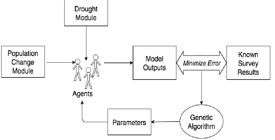
between model outputs and survey results (Figure 1). This chapter is organized as follows: first,
the survey data collection methodology is discussed; second, the ABM structure is presented;
third, a new drought module is described; next, the population growth module is presented; and
finally, the parameterization of the model with the GA is described.
Figure 1. A schematic of the GA-ABM interface
3.1 Survey Data Collection
Surveys were administered throughout an urban population center. To determine the
9 𝑆 = 𝑍2 𝑝(1−𝑝)
𝐶2 (3.1)
𝑆𝑎𝑑𝑗𝑢𝑠𝑡𝑒𝑑 = 𝑆
1+𝑆−1𝑃 (3.2)
where S is the sample size, Z is the z-score, p is the estimated value of the proportion of
population needed to be surveyed (p = 0.5 is most conservative assumption and is used when the
proportion is unknown), C is the confidence level, Sadjusted is the adjusted sample size, P is the
population size.
Neighborhoods were selected for this study based on their water supply’s original source
(groundwater or surface water) and to ensure the widest geographic coverage around the city.
Once neighborhoods were identified, survey administrators selected streets and homes from
those neighborhoods at random. Surveys were conducted on weekends to ensure better
representation of working citizens. If the occupant of a home was not available or declined to
take the survey, the next house was selected. For a thorough description of the survey
methodology and analysis of results, see Ramsey, Berglund, & Goyal (2017).
Identifying water-conservation behaviors is inherently difficult because many personal
water-consumption behaviors are unverifiable within a simple written survey, such as turning off
the tap when washing dishes. Consequently, this study explored the installation of dual-flush
toilets as a concrete measure of conservation behavior adoption. The two survey questions used
to parameterize this study based on dual-flush toilet installation:
1.) How many of each toilet do you have? a.) Dual-Flush
b.) Single-Flush c.) Pour-Flush d.) Other/don’t know
10 The responses to these questions were used to derive the expected number of WC agents at every
twelfth time step as follows:
𝑛𝑊𝐶,𝑡
𝑛𝑟𝑒𝑠𝑝𝑜𝑛𝑑𝑒𝑛𝑡𝑠 × 𝑁𝑡 = 𝑁𝑒𝑥𝑝𝑒𝑐𝑡𝑒𝑑 𝑊𝐶,𝑡 (3.3)
where nWC,tis the total number of survey respondents who had adopted dual-flush toilets by time
step t, nrespondentsis the total number of survey respondents, Nt is the total number of agents
interacting in the model at time t, and Nexpected WC, t is the number of expected WC agents at time
step t based on survey data.
3.2 ABM Framework
The framework presented here is an extension of the behavior diffusion ABM developed
by Young (1996) and expanded by Edwards et al. (2005) and Galán et al (2009).
Their framework models the diffusion of water conservation technology throughout a network of
agents. Agents are programmed as either adopters or non-adopters, and at each time step they
examine the adoption status of all of their neighbors and then compute the utility of updating
versus maintaining their adoption status. Agents then update their status based on the highest
utility. This research extends the model to include time delays in decision making and a separate
communication function that limits agents’ awareness of their neighbors’ behaviors. It also
incorporates drought and population growth modules and a Watts-Strogatz small world network
structure. The ABM is programmed in MASON, a Java-based discrete-event multi-agent
simulation library (Luke 2004) and presented in accordance with the ODD (Overview, Design
concepts, and Details) protocol introduced by Railsback and Grimm as a standardized method of
describing an ABM (Railsback and Grimm 2012). In the Overview section, the model purpose,
entities, state variables, temporal scales, and process overview and scheduling are introduced.
11 and objectives, sensing, interaction, stochasticity, and observation capabilities within the model
are discussed. In the Details section, the state of the model at initialization and inputs to the
model are described.
3.2.1 Overview
The purpose of the model is to simulate the spread of residential water conservation
behavior over time within a population and to evaluate the potential impacts it may have on
water demand. The entities in the model are agents, which each represent 100 households (to
reduce computational complexity). The agents have several state variables, which distinguish
entities from each other or trace how the entity changes over time. These include a binary
consumption behavior of either Water Conserver (WC) or Non-Water Conserver (NWC); a
weight for susceptibility to extrinsic pressures other than drought, eOTHER; a weight for
importance assigned to drought occurrence, eDROUGHT; a frequency of communication with
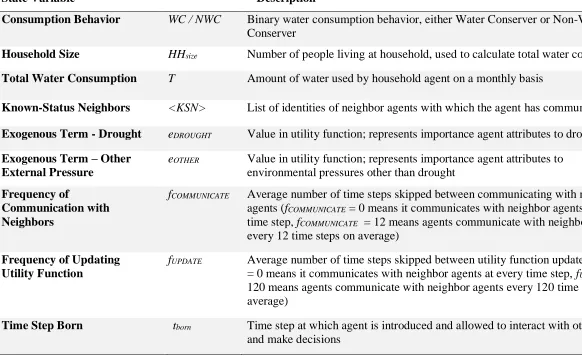
neighbors, fCOMMUNICATE; and a frequency of updating utility function, fUPDATE. A full list of the
12
Table 1. ABM state variables
State Variable Description
Consumption Behavior WC / NWC Binary water consumption behavior, either Water Conserver or Non-Water Conserver
Household Size HHsize Number of people living at household, used to calculate total water consumption
Total Water Consumption T Amount of water used by household agent on a monthly basis
Known-Status Neighbors <KSN> List of identities of neighbor agents with which the agent has communicated Exogenous Term - Drought eDROUGHT Value in utility function; represents importance agent attributes to drought
Exogenous Term – Other External Pressure
eOTHER Value in utility function; represents importance agent attributes to
environmental pressures other than drought Frequency of
Communication with Neighbors
fCOMMUNICATE Average number of time steps skipped between communicating with neighbor
agents (fCOMMUNICATE = 0 means it communicates with neighbor agents at every
time step, fCOMMUNICATE = 12 means agents communicate with neighbor agents
every 12 time steps on average) Frequency of Updating
Utility Function
fUPDATE Average number of time steps skipped between utility function updates (fUPDATE
= 0 means it communicates with neighbor agents at every time step, fUPDATE =
120 means agents communicate with neighbor agents every 120 time steps on average)
Time Step Born tborn Time step at which agent is introduced and allowed to interact with other agents
13 The process overview and scheduling of the model, which are repeated at each time step,
are outlined below.
Step 1:
The model calls the population module and determines how many agents have a tborn at the
current time step, and then introduces them into the population. Once introduced, agents are
allowed to interact and update their own behaviors.
This population module adds to the Edwards model, which keeps population static.
Galan’s model includes population growth, but the social network structures differ between this
approach and Galan’s model, which results in a difference in the way agents are introduced.
Step 2:
The model calls the drought module to determine if the previous year was a drought and sets the
dummy drought variable, d, to 1 or 0 if the previous year was a drought or was not a drought,
respectively. This module is a new extension of the Edwards model.
Step 3:
Each agent determines whether it communicates with a neighbor at the current time step as
follows:
IF 𝑥 ≤ 1/𝑓𝐶𝑂𝑀𝑀𝑈𝑁𝐼𝐶𝐴𝑇𝐸 THEN:
FOR all neighbors of current agent:
Select a random agent from neighbors
IF selected neighbor agent 𝑡𝑏𝑜𝑟𝑛 ≤ 𝑡 THEN:
IF selected neighbor agent is not in <KSN>THEN: Add neighbor agent to <KSN>
14 Exit loop
where x is a randomly selected number in the interval [0,1). Agents are allowed to communicate
only with agents that have a tbornless than or equal to than the current model time step. It the
selected agent has a higher tborn,(i.e. it has not been introduced yet), then it is discarded and the
agent iterates through neighbor agents randomly until either an agent with a lower tbornis found
or all neighbors have been discarded, at which point the next agent starts Step 3. The ability of
agents to decide when to communicate with other agents and the limited scope of their awareness
of their neighbors’ behaviors is an adaptation of the Edwards model.
Step 4:
Each agent determines whether it updates its utility functions at the current time step. For a given
agent, A, 𝜈𝐴(𝑊𝐶 → 𝑊𝐶) is the utility of maintaining WC behavior, 𝜈𝐴(𝑊𝐶 → 𝑁𝑊𝐶) is the
utility of switching from WC to NWC behavior, 𝜈𝐴(𝑁𝑊𝐶 → 𝑊𝐶) is the utility of switching from
NWC to WC behavior, and 𝜈𝐴(𝑁𝑊𝐶 → 𝑁𝑊𝐶) is the utility of maintaining NWC behavior. The
agent computes if it should update its utility functions and, if so, calculates them as follows:
IF WC:
IF 𝑥 ≤ 1/𝑓𝑈𝑃𝐷𝐴𝑇𝐸 THEN:
𝜈𝐴(𝑊𝐶 → 𝑊𝐶) = 𝑎 ∙ 𝑉(𝐴, 𝑊𝐶) + 𝑒𝑂𝑇𝐻𝐸𝑅+ 𝑑 ∙ 𝑒𝐷𝑅𝑂𝑈𝐺𝐻𝑇 (3.4)
𝜈𝐴(𝑊𝐶 → 𝑁𝑊𝐶) = 𝑏 ∙ 𝑉(𝐴, 𝑁𝑊𝐶) (3.5)
ELSE:
IF 𝑥 ≤ 1/𝑓𝑈𝑃𝐷𝐴𝑇𝐸 THEN:
𝜈𝐴(𝑁𝑊𝐶 → 𝑊𝐶) = 𝑎′∙ 𝑉(𝐴, 𝑊𝐶) + 𝑒
𝑂𝑇𝐻𝐸𝑅+ 𝑑 ∙ 𝑒𝐷𝑅𝑂𝑈𝐺𝐻𝑇 (3.6)
15 where x is a randomly selected number from the interval (0,1], a and a' are the weights used to
evaluate conservation behavior when Agent A is a WC or WNC, respectively; b and b' are the
weights used to evaluate non-conservation behavior when Agent A is a WC or NWC,
respectively; 𝑉(𝐴, 𝑊𝐶) is the ratio of WCs within their Known Status Neighbor list, <KSN>, to
total number of neighbors; 𝜈(𝐴, 𝑁𝑊𝐶) is is the ratio of NWCs within <KSN> and assumed NWC
neighbors to the total number of neighbors, and d is a dummy variable (d = 1 if previous year
was a drought year, d = 0 otherwise). Agents assume that any agent with which they have not
communicated exhibits a NWC behavior when calculating these ratios.
This approach builds on the Edwards and Galan models by designating two separate
exogenous terms eDROUGHT and eOTHER, to represent a change in external pressures due to
climatological changes. The approach also separates the communication function from the utility
update function and implements a delay in both functions to represent the delays involved in
deciding to adopt dual-flush toilets, due to their expense and the effort required to install them.
Step 5:
To allow for some stochasticity in the model, the agent calculates a probability function based on
the utility function and updates its behavior with probability P. P(WC→WC) and P(NWC→NWC)
are the probabilities of maintaining current WC or NWC behavior, respectively. P(WC→NWC)
and P(NWC→WC) are the probabilities of switching behaviors, either from WC to NWC or NWC
to WC, respectively. The probability functions are as follows:
IF WC THEN:
P(WC→WC) = 𝑒𝛽∙𝜈𝐴(𝑊𝐶→𝑊𝐶)𝑒𝛽∙𝜈𝐴(𝑊𝐶→𝑊𝐶)+𝑒𝛽∙𝜈𝐴(𝑊𝐶→𝑁𝑊𝐶) (3.8)
P(WC→NWC) =𝑒𝛽∙𝜈𝐴(𝑊𝐶→𝑊𝐶)𝑒𝛽∙𝜈𝐴(𝑊𝐶→𝑁𝑊𝐶)+𝑒𝛽∙𝜈𝐴(𝑊𝐶→𝑁𝑊𝐶) (3.9)
16
P(NWC→WC) = 𝑒𝛽∙𝜈𝐴(𝑁𝑊𝐶→𝑊𝐶)𝑒𝛽∙𝜈𝐴(𝑁𝑊𝐶→𝑊𝐶)+𝑒𝛽∙𝜈𝐴(𝑁𝑊𝐶→𝑁𝑊𝐶) (3.10)
P(NWC→NWC) =𝑒𝛽∙𝜈𝐴(𝑁𝑊𝐶→𝑊𝐶)𝑒𝛽∙𝜈𝐴(𝑁𝑊𝐶→𝑁𝑊𝐶)+𝑒𝛽∙𝜈𝐴(𝑁𝑊𝐶→𝑁𝑊𝐶) (3.11)
where ß is a measure of the randomness of Agent A’s decision-making process. If ß = 1, the
process is completely stochastic, and if ß = 100, the process is largely deterministic.
Step 6:
The model aggregates data about the number of WC agents, total monthly water consumption
(T), the number of total agents, and the ratio of all WC agents to the total number of agents. T is
calculated as follows:
𝑇 = ∑𝑚𝑁𝑊𝐶𝐻𝐻𝑠𝑖𝑧𝑒𝑖 ∙ 𝐷
𝑖=0 + ∑𝑛𝑗=0𝑊𝐶𝐻𝐻𝑠𝑖𝑧𝑒𝑗(𝐷 − 𝑤𝑠) (3.12)
where mNWC and nWCare the number of WC and NWC agents at time step t, respectively, D is the
expected monthly demand used by water resource managers, and ws is the expected monthly
water savings generated from water conservation behavior adoption.
3.2.2 Design
Basic Principles: The model is an adaptation of the innovation diffusion model, which is often
used to simulate the adoption of technology within a population. This design incorporates
population growth and an element of timing in decision making and communication about
technology to allow for a closer approximation to reality.
Emergence: The interactions between water consumer agents drive the emergence of
conservation technology adoption.
Adaptation, learning and objectives: The water consumer agents have rules of adaptation based
on utility functions. The utility functions are designed to meet the agents’ objectives of adhering
to social norms and responding to external pressures, but they do not optimize any objective
17
Sensing: The consumer agents sense the behaviors of members of their social networks with
whom they have communicated at each time step after communication.
Interaction: Consumer agents are all connected via a Watts-Strogatz small world network, using
the GraphStream library (Balev et al. 2015). Agents store identities of known-status neighbors
and then check their status every time they recalculate their utility functions and reevaluate their
behavior. This network structure was added to the Edwards model.
Stochasticity: Stochasticity occurs in the model due to several factors: the decision to update
behavior based on a probability function, the connections between agents, the timing of
communication and updating of the utility function, and the order of agents selected to
communicate.
Observation: Results of the model are observed as the number of agents exhibiting WC behavior,
the number of agents introduced, the ratio of WC to total number of agents, assumed water
consumption, and assumed water savings. Results are collected at the end of each time step, after
all agents have completed their interactions.
3.2.3 Details
The model creates an entire population of agents equal to the maximum number of agents
for the scenario at initialization. All agents are assigned a conservation behavior of NWC, and a
household size drawn from a Poisson distribution with an average value taken from census data.
If the household size drawn is <1, then another household size is drawn. Agents are also assigned
a frequency of communicating with other agents, fCOMMUNICATE, and a frequency of updating their
utility functions, fUPDATE, drawn from Poisson distributions with an average of fcommunicate and
fupdate, respectively. The values for fcommunicate and fupdate are determined by the GA. If fCOMMUNICATE
18 values eDROUGHTand eOTHER, drawn from a normal distribution with standard deviations of 0.1
and an average of edrought and eother, respectively, which are also determined by the GA.
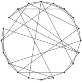
All agents are added as nodes to a Watts-Strogatz small world network (Figure 2). A
small world network consists of a ring of n nodes, each of which is connected to its k nearest
neighbors in the ring, and each of those nodes is rewired to another random node with a
probability of ßrewire. Each agent is assigned a time step, tborn, at which it is allowed to begin
interacting with other agents and making behavior decisions.
Figure 2. Watts-Strogatz small world network structure
The ABM reads in inputs from a precipitation sub-model every year (every twelfth time
step), and inputs from a population growth projection every month (each time step), which is
used to set tborn for each agent. If, for example, a total population of 100 agents is created and 10
agents are to be introduced at each time step, 10 agents would be assigned a tborn = 0, 10 agents
would be assigned tborn = 1, and so on. The agents with tborn = 1 only interact or update their
19 3.3 Population Growth Module
The population growth module uses linear interpolation to derive population increase or
decrease from census data, and then calculates the corresponding number of agents. The number
of agents at each time step is determined by:
𝑛𝑡= ℎℎ∙100𝑝𝑡 (3.13)
where ntis the number of agents with tborn ≥ t at time step t, pt is the population at time t, and hh
is the average household size. ptis divided by 100 to reduce computational complexity.
3.4 Drought Module
When called at each time step representing the beginning of a new year (every twelfth
time step), the drought module determines if the previous year was a drought year by the
following equation:
IF t/12 = 1 THEN: IF ∑𝑖= 12𝑝𝑡−𝑖
𝑖=1 ≤ 0.75𝑝𝑎𝑣𝑔 THEN:
d = 1
ELSE:
d = 0
where pt=iis precipitation at time step t - i, pavg is the long-term average precipitation, and d is
the dummy variable for drought used in the agents’ utility functions.
3.5 Parameterization with Genetic Algorithm
The ABM was parameterized using a GA which is implemented in Java and has been
applied to solve a range of environmental and water resources planning and simulation problems
20 rules at each generation to converge to an optimal or near-optimal solution. A solution is an array
of decision variables that can have binary, real, or integer values. After each generation of
solutions is created, the best performing solutions are selected for crossover, in which decision
values from the best performing solutions are combined to produce another generation of
solutions. Mutation is also applied, which makes random changes to existing solutions. This
approach uses a noisy GA, which is a GA that uses an average of fitness function values in order
to operate in a noisy or uncertain environment (Miller and Goldberg 1996).
A solution is represented as an array of six real-valued parameters. The GA is applied to
identify ABM parameters over a range of potential values (Table 2). The decision variable brep is
transformed to the parameter b in the ABM using Eqn. 3.14 to enforce that b is less than or equal
to a.
𝑏 = 𝑏𝑟𝑒𝑝× 𝑎 (3.14)
The parameters corresponding to the weights attributed to the same behaviors, a and b’, and
opposite behaviors, a’ and b, are set equal to each other (Eqn. 3.15 and 3.16), as was done in the
Galan and Edwards models.
𝑎 = 𝑏′ (3.15)
𝑏 = 𝑎′ (3.16)
Each solution is simulated for five random realizations, and the average standard error of
the regression, S, between the model outputs and the survey data is reported as the objective
function, which is minimized. S is used to represent error because it can be used to determine
error in non-linear models, and S is given in the same units as the model output, which is the
21
Table 2. Parameter ranges for the ABM set by the GA
Parameter Allowable Value Range
a 0 – 1
brep 0 – 1
eother 0 – 1
edrought 0 – 1
fcommunicate 0 – 36
22
CHAPTER 4: CASE STUDY—THE CITY OF JAIPUR
Jaipur is the capital and largest city in the state of Rajasthan in northwest India. It was
selected as a case study because it is both severely water stressed and growing rapidly, with an
annual growth rate of 5.3%. Jaipur’s population in 2011 was approximately 3.1 million, more
than triple its population in 1981 (Office of the Registrar General & Census Commissioner
2011). Projections of Jaipur’s population growth vary widely; the Jaipur Development Authority
(JDA), which is charged with planning for Jaipur’s development, projects the population will
grow to 6.5 million by 2025. Alternatively, the most aggressive projections from the Global
Cities Institute (GCI), which are based on the United Nations World Urbanization Prospects,
project the population will reach only 4.3 million by 2025, but hit 11.0 million by 2100. For this
model, the JDA projections for 2025 and the GCI projections for 2050 to 2100 are combined (see
Figure 3). This approach creates a lower growth rate for the time period between 2025 to 2050
than that of the GCI projections, but allows consistency with city plans.
Figure 3. Population data and projections for Jaipur City, 1991-2100
0 2 4 6 8 10 12
1991 2001 2011 2025 2050 2075 2100
Popul
at
ion
(in mi
lli
ons
)
Year
23
Figure 4. Location of Jaipur, India
The Public Health Engineering Department- Rajasthan (PHED) provides water to most of
Jaipur’s citizens. PHED draws water from the Bisalpur Reservoir and from 1897 wells
distributed throughout the city (Public Health Engineering Department 2011). The Bisalpur
Reservoir, which became operational in 2009, lies on the Banas River, a seasonal river that often
does not flow during the dry season. Previously, Jaipur’s water supply came from Ramgarh
Lake, which was created in the 1890s, but dried up in the late 1990s due to mismanagement and
excessive upstream diversions (Bhandari et al. 2012). Jaipur relied solely on groundwater to
meet its water demands during the interim between 1999 and 2009. According to a government
audit, Bisalpur Reservoir has only 40% dependability; that is, only 40% of the designed capacity
of the dam (317.2 million m3) can be expected to be continuously available under drought
conditions (Accountant General 2010). Consequently, PHED still relies heavily on groundwater
to meet Jaipur’s water demands, particularly when monsoon rains are low. Estimates show that
24 and in some areas of Jaipur District the groundwater table has dropped by over 25 meters since
2001 (“Jaipur: Groundwater table sinks 25 metres in 10 yrs” 2015).
Water supply is intermittent, and the majority of residents have access to running water
for less than two hours per day. Many residents cope with this intermittency by storing water in
tanks to use throughout the day. Select neighborhoods have been receiving 24-hour water supply
in 2011 as part of a pilot project. A small percentage of residents do not use PHED-supplied
water, relying instead on private wells. Wealthier residents often have both a PHED water
connection and a private well, which they use when PHED-supplied water does not meet
household demands.
The climate in Jaipur is semi-arid. Jaipur receives an annual average of 600.1 mm of rain
a year, 88.5% of which falls during the monsoon season (Government of Rajasthan 2016),
defined by the Indian Meteorological Department as June 1 to September 30. On average, Jaipur
experiences a drought (less than 75% of the long term average rainfall, or 450.1 mm) at least
25
Figure 5. Precipitation in Jaipur City (1957-2015) 0
200 400 600 800 1000 1200 1400
1957 1959 1961 1963 1965 1967 1969 1971 1973 1975 1977 1979 1981 1983 1985 1987 1989 1991 1993 1995 1997 1999 2001 2003 2005 2007 2009 2011 2013 2015
Preci
pi
ta
tio
n
(mm)
26
CHAPTER 5: RESULTS
5.1 Survey Results
A household survey was conducted on 248 households within Jaipur, India in 2015
(Figure 6). Responses on the year of installation of dual-flush toilets are shown in Figure 7.
Responses in which participants did not know the date of installation were not included in the
parameterization process. Because the model measures the installation of dual-flush toilets, a
decision that is irreversible for the life of the technology, once agents adopt WC behavior, they
do not update their utility function again.
The average assumed water savings, ws, per person are calculated as follows:
𝑤𝑠 = 5.1 × (6.06 − 4.54) = 7.75 𝑙𝑝𝑐𝑑 (5.1)
based on dual flush toilet data (Table 3).
27
Figure 7. Number of households adopting dual-flush toilets in Jaipur City, India by year
Table 3. Water demand data (Jaipur Development Authority 2011; McMordie-Stoughton et al. 2005; Vickers 2001)
Per Capita Demand 200 liters/person/day
Dual Flush Toilet Water Consumption 4.54 liters/flush
Regular Flush Toilet Water Consumption 6.06 liters/flush
Average Number of Flushes 5.1 flush/person/day
5.2 Initialization of the ABM
For parameterization, the model is initiated in January 1997 and ends at December 2015.
Using linear interpolation from census data, the population size at January 1997 is assumed to be
2.04 million, and 4.31 million at December 2015 (Office of the Registrar General & Census
Commissioner 2011). 8280 agents are initialized for the duration of the model, with 3,922 given
28 Agents are assigned a household size from a Poisson distribution with an average size of
5.2, which is the average urban household size in Jaipur (Office of the Registrar General &
Census Commissioner 2011), with a maximum size of 20 and a minimum of 1.
The Watts-Strogatz small world network is given an average number of connections of
k=48, and an average rewiring probability ß = 0.25, based on a social network study conducted in
southern India (Shakya et al. 2014).
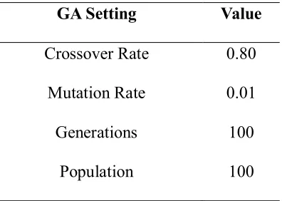
5.3. Genetic Algorithm Performance
The GA was run for five independent trials to parameterize the ABM using algorithmic
settings shown in Table 4. The results of the GA trials are listed in Table 5, ordered from best to
worst performance. The best set of parameters generated by the GA has a standard error of S =
574.403. The fitness convergence (as measured by S) of each of the five optimal parameter sets
for each generation is shown in Figure 8. The GA identifies a good solution early in the search
and makes minor improvements throughout the rest of the search. Each GA trial takes an
average of 12.8 hours to complete with the settings given in Table 4.
The GA was re-run for a single trial with a population of 1000 and five generations to
assess whether increasing the number of chromosomes allows a better exploration of the problem
space. While this approach generated marginal improvement in the model fitness, the returns for
the added computational time required (35.8 hours vs 12.8 hours per trial) are of negligible
29
Table 4. GA settings and values
GA Setting Value
Crossover Rate 0.80
Mutation Rate 0.01
Generations 100
Population 100
Table 5. Parameters generated by GA for independent trials
GA
Trial # a b eother edrought fcommunicate fupdate
Standard Error of the Regression
Number of Runs to Convergence
1 0.803 0.333 0.516 0.129 2 141 574.403 9887
2 0.955 0.310 0.725 0.112 7 154 576.073 9913
3 0.784 0.378 0.544 0.098 5 171 582.474 9892
4 0.449 0.192 0.276 0.042 10 148 592.994 9882
30
Figure 8. Fitness of parameter sets generated by GA, as measured by S
The ABM was executed for 30 random simulations using each of the GA-generated
parameter sets to assess stochasticity in the model’s performance. The average results from these
trials are presented alongside the household survey in Figure 9 as a number of raw agents and in
Figure 10 as a percentage of the total number of agents. The model performs well at the
beginning of each of the runs, but fails to keep pace with the real world reported adoption rate
that increased around 2013, suggesting that another driver of adoption behavior exists which is
not represented by social pressures, external pressure, and responses to drought. One possible
driver could be an increase in water awareness following the failure of Jaipur’s former surface
water source, Ramgarh Lake, to refill even during heavy monsoons in 2012 (Singh 2012).
550 560 570 580 590 600 610 620 630
0 10 20 30 40 50 60 70 80 90
S
Generation
31
Figure 9. Average number of conserver agents for 30 simulations of parameter sets 1-5
Figure 10. Average percentage of population as water conservers for 30 simulations of
parameter sets 1-5
The relationship between the model’s fitness and the six variables parameterized by the
GA (a, b, edrought, eother, fupdate, and fcommunicate) as found for Trial 1 were explored to identify the
ranges of parameters with the best performance and to analyze potential drivers behind the GA’s
behavior. The S values for each permutation within the GA are plotted against each of the
0 500 1000 1500 2000 2500 19 97 19 98 19 99 20 00 20 01 20 02 20 03 20 04 20 05 20 06 20 07 20 08 20 09 20 10 20 11 20 12 20 13 20 14 20 15 N umbe r of C ons er ver A gent s Year
Set 1 Set 2 Set 3 Set 4 Set 5 Survey results
0% 5% 10% 15% 20% 25% 30% 19 97 19 98 19 99 20 00 20 01 20 02 20 03 20 04 20 05 20 06 20 07 20 08 20 09 20 10 20 11 20 12 20 13 20 14 20 15 Cons er vers a s P er ce nt ag e of T ot al Ag ent s Year
32 variables in Figures 11-16. The ranges of the GA-generated parameters with the best solutions (S
< 1000) are given in Table 6.
Table 6. Ranges of parameters for the best solutions generated by GA Trial 1
Parameter Range
a 0.400-1.000
b 0.172-0.578
eother 0.067-0.613
edrought 0.018-0.501
fcommunicate 1-36
fupdate 12-179
The best performing values for a, the weight given to agents exhibiting the same behavior
as the agent updating its utility function, are greater than 0.400 (Figure 11). The best performing
values for b, the weight given to agents exhibiting the opposite behavior, are less than 0.578
(Figure 12). The best performing range for a - b was determined to be between0.109 and 0.531.
The best performing values of eotherrange from 0.067 to 0.613, and the best performing values of
edroughtrange from 0.018 to 0.501. The best performing range for the sum of eotherand edrought is
between 0.308 and 0.742 (Figures 13 and 14, respectively). The best performing range for eother-
edroughtis -0.419 to 0.484, indicating that the model is not limited by which parameter is larger.
The best performing values of fcommunicate range across the GA constraints of 1 to 36; the values
thus do not appear to impact the model performance significantly (Figure 15).
Similarly, the best fupdate values fall along the GA constraint range, from 12 to 179. As
seen in Figure 16, a clear relationship between fupdate and the range of S values (Srange) exists, and
33 𝑆𝑟𝑎𝑛𝑔𝑒 = 0.0618𝑓𝑢𝑝𝑑𝑎𝑡𝑒2 − 28.695𝑓
𝑢𝑝𝑑𝑎𝑡𝑒+ 4992.5 (5.1)
with an R2=0.919. This relationship shows that the permutations within the GA all have a lower
range of error as fupdate increases. The minimum value for Srange = 1661.582, occurs when when
fupdate = 232.160 (19.3 years). This is due to the dominance of the fupdate parameter as it increases.
When fupdate is low, the agents update their utility functions and behaviors more often.
Consequently, they are more likely to adopt WC behavior early in the model, which yields a
higher S value when compared to the slower real world adoption rate. As fupdate increases,
regardless of the other parameters, the slower adoption rate reduces the error of the model. There
are, however, some permutations with a low fupdate that have a relatively low error, indicating that
while fupdate dominates the model, the other parameters continue to play a contributing role in
34
Figure 11. Relationship between a and S for each chromosome in GA Trial 1
Figure 12. Relationship between b and S for each chromosome in GA Trial 1
0 500 1000 1500 2000 2500 3000 3500 4000 4500 5000
0 0.1 0.2 0.3 0.4 0.5 0.6 0.7 0.8 0.9 1
S
a
0 500 1000 1500 2000 2500 3000 3500 4000 4500 5000
0 0.1 0.2 0.3 0.4 0.5 0.6 0.7 0.8 0.9 1
S
35
Figure 13. Relationship between eother and S for each chromosome in GA Trial 1
Figure 14. Relationship between edrought and S for each chromosome in GA Trial 1
0 500 1000 1500 2000 2500 3000 3500 4000 4500 5000
0 0.1 0.2 0.3 0.4 0.5 0.6 0.7 0.8 0.9 1
S
eother
0 500 1000 1500 2000 2500 3000 3500 4000 4500 5000
0 0.1 0.2 0.3 0.4 0.5 0.6 0.7 0.8 0.9 1
S
36
Figure 15. Relationship between fcommunicate and S for each chromosome in GA Trial 1
0 500 1000 1500 2000 2500 3000 3500 4000 4500 5000
0 5 10 15 20 25 30 35 40
S
37
Figure 16. Relationship between fupdate and S for each chromosome in GA Trial 1, by select generation number 0
500 1000 1500 2000 2500 3000 3500 4000 4500 5000
12 32 52 72 92 112 132 152 172
38 5.4 Simulation Using Parameter Set 1
Using the highest performing set of parameters (Set 1), adoption rates were projected to
2100. Droughts are modeled using the historical record up to the year 2015 and are generated
randomly starting in 2016, assuming a rate of drought occurrence consistent with the current rate
(29.3%). Thirty simulations were run, and the average number and range of WC adopters at each
time step are presented in Figure 17. The number of total agents is included in the graph for
reference. The different model simulations generate a range in the number of adopters beginning
in 2015, when the random drought generation module starts, indicating that the order in which
droughts occur within the model plays a role in adoption rates. The maximum range reaches
3815 agents (29.0% of total agents at that time step) in February 2042. The model never reaches
100% adoption because new agents are introduced to the model as NWC agents, preventing
universal adoption.
Figure 17. Range of performance for WC behavior adoption projection, 1997-2100
0 5000 10000 15000 20000 25000 19 97 20 02 20 07 20 12 20 17 20 22 20 27 20 32 20 37 20 42 20 47 20 52 20 57 20 62 20 67 20 72 20 77 20 82 20 87 20 92 20 97 N um be r o f W C Agen ts Year
39 A comparison between the average monthly projected water demand for Jaipur City from
the model and projected water demand based on static per capita demand is shown in Figure 18,
and the difference between the two is shown in Figure 19. According to the model, water savings
generated by adoption of WC behaviors will reach 2.3 billion liters of water per month will by
2100, or roughly 3.5% of static per capita demand.
Figure 18. Monthly projected water demand for Jaipur City
0 10 20 30 40 50 60 70 80 19 97 20 02 20 07 20 12 20 17 20 22 20 27 20 32 20 37 20 42 20 47 20 52 20 57 20 62 20 67 20 72 20 77 20 82 20 87 20 92 20 97 W ater D em an d (in b ill io ns of li ter
s p
er m on th ) Year
40
Figure 19. Difference in water demand between model and static per capita demand
In Figure 20, the results from the 30 simulations run with Parameter Set 1 with the
highest and lowest number of adopters as well as the average performance are presented. The
greatest difference between the best and worst performing simulations occurs at February 2043,
with a difference of 2207 WC behavior adopter agents (16.7% of the total number of introduced
agents). By October 2095, the difference between the best and the worst performance reaches
<2% of the total number of agents. Thus, while there is significant stochasticity within the
middle of the simulation, the performance is similar at the end.
0 0.5 1 1.5 2 2.5 19 97 20 02 20 07 20 12 20 17 20 22 20 27 20 32 20 37 20 42 20 47 20 52 20 57 20 62 20 67 20 72 20 77 20 82 20 87 20 92 20 97 W ater Sa vi
ngs (
41
Figure 20. Adoption of WC behavior--best, worst, and average performances
Figure 21 shows the rate of adoption in agents/month for the three simulations shown in
Figure 20 (lowest adoption, highest adoption, and average performance). The population growth
rate is also shown, in new agents/month. The population growth rate between 2025 and 2050
drops as a result of the combination of the JDA and GCI population projections (as shown in
Figure 3). Visualizing the rate of adoption and rate of population change, rather than cumulative
values alone, provides another set of insights into the performance of the model.
At the beginning of the model, adoption rates are driven predominantly by the statically
programmed drought conditions (denoted by red bands). When drought conditions are not
present early in the model, adoption rates are close to zero. As more agents adopt WC behavior,
the rate of adoption increases towards the middle of the simulation, and the primary driver of this
spread becomes the social pressure from neighboring agents. Although the population growth
rate drops between 2025 and 2050, the rate of adoption continues to increase as many of the
0 5000 10000 15000 20000 25000 19 97 20 02 20 07 20 12 20 17 20 22 20 27 20 32 20 37 20 42 20 47 20 52 20 57 20 62 20 67 20 72 20 77 20 82 20 87 20 92 20 97 N um be r o f C on vs er ver s Year
42 newly introduced NWC agents begin to adopt WC behavior. The rate of change curve shown in
Figure 21 demonstrates the characteristics that lead to a typical S-shape curve, as expected for
technology adoption diffusion. Toward the end of the projected period, the rate of adoption does
not return to zero, but it is approximately equal to the rate of population change.
The best performing simulation has a maximum adoption rate of 52 agents per month,
which it achieves at two time steps: May 2040 and February 2041. The average of all simulations
reaches its peak at 32.03 agents/month in September 2039, and the poorest performing
simulation reaches its peak of 48 agents/month in May 2044. While the rates between the best
and the worst performers are close in magnitude, the four-year delay could result in higher
aggregate water use. The earlier high adoption rates in the best performing simulation are likely
due to the order of drought occurrence generated by the drought module. During the
top-performing simulation, the drought module generated consecutive droughts from 2015 to 2017,
which caused more agents to adopt at the beginning of the model and pushed the model towards
43
Figure 21. Rate of WC behavior adoption, 1997-2100
0 10 20 30 40 50 60
1997 2002 2007 2012 2017 2022 2027 2032 2037 2042 2047 2052 2057 2062 2067 2072 2077 2082 2087 2092 2097
Ra
te
of
A
do
pti
on
(A
gen
ts
/Mo
nth
)
Year
44 5.5 Simulation Using Various Drought Scenarios
The model was run for four drought scenarios: Dry (58.6% annual likelihood of drought,
double the current drought rate), Very Dry (87.9% annual likelihood of drought, triple the
current drought rate), Perpetual Drought (a drought occurs for the entire duration of the model),
and Wet (no drought occurs for the duration of the model). The Perpetual Drought and Wet
scenarios are climatologically improbable, but are used here to explore the sensitivity of the
model to changes in drought frequency. Each scenario was modeled using the ABM for 30
random simulations and the average results are presented alongside the Stationary Climate
scenario (presented in Section 5.5) in Figure 22.
Figure 22. WC behavior adoption under varying drought scenarios
For the Dry, Very Dry, and Perpetual Drought scenarios, adoption rates are higher than
the Stationary Climate scenario. The maximum differences in WC adoption numbers are given in
Table 7. The maximum difference between the Stationary Climate and the Perpetual Drought
0 5000 10000 15000 20000 25000 19 97 20 02 20 07 20 12 20 17 20 22 20 27 20 32 20 37 20 42 20 47 20 52 20 57 20 62 20 67 20 72 20 77 20 82 20 87 20 92 20 97 N um be r o f A gen ts Year
Total Number of Agents Stationary Climate Wet
45 scenario occurs eight time steps earlier in the model than the Very Dry scenario, but there is only
a 2.0% difference in agents adopting WC behavior. The small difference between the two is
likely due to the already high drought occurrence within the Very Dry scenario. The maximum
difference between the Wet scenario and the Stationary Climate scenario is greater than 50% of
the population, or number of agents that exist, at that time step, and occurs close to the end of the
simulation. This demonstrates that the presence of the drought module is a key driver of the WC
adoption behavior in the model. Again, the model never achieves 100% adoption even in the
Perpetual Drought scenario because of the continued introduction of NWC agents into the model
to simulate population change.
Table 7. Maximum difference in WC adoption between drought scenarios and Stationary
Climate scenario and time step of occurrence
Scenario
Maximum Difference/
Percentage of Total Agents Time Step of Occurrence
Dry 2133.8 (16.3%) February 2041
Very Dry 3416.1 (26.2%) October 2037
Perpetual Drought 3669.3 (28.2%) February 2037
46
Figure 23. WC behavior adoption rate under varying drought scenarios
0 5 10 15 20 25 30 35 40 45
1997 2002 2007 2012 2017 2022 2027 2032 2037 2042 2047 2052 2057 2062 2067 2072 2077 2082 2087 2092 2097
W
C B
eh
avi
or
A
do
pter
s/
Mo
nth
Year
47
Table 8. Maximum rate of WC behavior adoption in drought scenarios and time step of
occurrence
Scenario Maximum Rate (Agents/Month) Time Step of Occurrence
Dry 38.5 September 2035
Very Dry 40.4 August 2027
Perpetual Drought 42.1 October 2027
Wet 20.8 November 2099
Stationary Climate 32.0 September 2039
The rates of WC behavior adoption (shown in Figure 23) diverge immediately as the
drought scenarios begin in 2015, and converge to less than one agent/month rate difference in
September 2064 in the model for the three driest scenarios. The maximum adoption rates for the
scenarios and the Stationary Climate Scenario are presented in Table 8. The three dry scenario
adoption rates are all within <4 agents/month of each other. However, the time scale varies
between the scenarios. The Perpetual Drought scenario maximum adoption rate occurred two
time steps after the Very Dry scenario maximum adoption rate was achieved. In contrast, the
maximum rate for the Dry scenario occurred 97 time steps later than the Very Dry scenario. This
indicates that a threshold exists beyond which an increase in drought frequency has minimal
impact on the adoption rate’s magnitude or timing.
WC behavior adoption continues in the Wet scenario due to the presence of social
pressure, but it is outpaced by the rate of population change. The maximum adoption rate is
achieved two time steps before the end of the simulation; it is likely that a higher rate would be
obtained after 2100 if the simulation had continued, as social pressure begins to dominate agent
utility functions. The performance of the model during the Wet scenario indicates that edrought is a