American
Society of Range Management
OFFICERS OF THE SOCIETY PRESIDENT
E. J. DYKSTERHUIS Texas A&M University College Station, Texas 77843
PRESIDENT ELECT DONALD A. Cox Mullen, Nebraska 69152
PAST PRESIDENT C. WAYNE COOK Utah State University Logan, Utah 84321
EXECUTIVE SECRETARY FRANCIS T. COLBERT
P. 0. Box 13302 Portland, Oregon 97213
(503) 284-5052
BOARD OF DIRECTORS 1966-68 MARTIN H. GONZALEZ Ranch0 Experimental La Campana
Apdo. Postal 682 Chihuahua, Chih., Mexico CHARLES E. POULTON Oregon State University Corvallis, Oregon 97331
1967-69
SHERMAN EWING S N Ranch P. 0. Box 160 Claresholm, Alberta LAURENCE E. RIORDAN
940 E. 8th Ave. Denver, Colorado 80218
1968-70
RAYMOND M. HOUSLEY, JR. U. S. Forest Service
P. 0. Box 1268 Flagstaff, Arizona 86002 ROBERT E. WILLIAMS
6403 Landon Lane Bethesda, Md. 20034
JOURNAL OF RANGE MANAGEMENT The Journal, published bimonthly, is the
official organ of the American Society of Range Management. The Journal aims to publish something of interest to the entire membership in each issue. The Society, however, assumes no responsibility for the statements and opinions expressed by au- thors and contributors.
Subscriptions. Correspondence concerning subscriptions, purchase price of single copies and back issues, and related business should be addressed to the Executive Sec- retary, P. 0. Box 13302, Portland, Oregon 97213. Subscriptions are accepted on a cal- endar year basis only. Subscription price is $15.00 per year in the U. S. and insular possessions, Canada and Mexico: $15.50 in other places. Checks should be made pay- able to the American Society of Range Man- agement. Subscribers outside the United States are requested to remit by Interna- tional Money Order or by draft on a New York bank.
Address Change. Notice of change of ad- dress should be received by the Executive Secretary prior to the first day of the month of Journal issue. Lost copies, owing to change of address, cannot be supplied unless adequate notice has been given. Missing Journals. Claims for missing copies of the Journal should be sent to the Executive Secretary within 60 days of pub- lication date. Such claims will be allowed only if the Society or the printing company is at fault.
Membership Dues. Dues for regular mem- bers are $15.00 per year in the United States, Canada, and Mexico, $15.50 else- where. Student memberships are $7.50 per year. Dues include a subscription to the Journal. Remittance must be in U. S. funds.
Post Office Entry. Second-class postage paid at Portland, Oregon, and at addi- tional offices.
Manuscripts. Address manuscripts and correspondence concerning them to the Editor, Journal of Range Management. In- structions to authors appear in the March Journal. Copies are available in the Edi- tor’s office.
Reprints. Reprints of papers in the Jour- nal are obtainable only from the authors or their institutions.
News And Notes. Announcements about meetings, personnel changes, and other items of interest to Society members should be sent directly to the Executive Secretary. Printers. Allen Press, Inc., 1041 New Hampshire Street, Lawrence, Kansas 66044. Copyright 1968 by the American Society of Range Management.
EDITOR ROBERT S. CAMPBELL
RR7 Quincy, Illinois 62301
(217) 223-7936
EDITORIAL BOARD 1966-68
ALAN A. BEETLE University of Wyoming Laramie, Wyoming 82071 CHARLES L. LEINWEBER
Texas A&M University College Station, Texas 77843
FRANK W. STANTON Bureau of Land Management
P. 0. Box 3861 Portland, Oregon 97208
1967-69
LORENZ F. BREDEMEIER Soil Conservation Service
P. 0. Box 4248 Madison, Wisconsin 53711
JACK F. HOOPER Utah State University Logan, Utah 84321 WILLIAM J. MCGINNIES U.S.D.A., Agricultural Res. Serv.
Colorado State University Fort Collins, Colorado 80521
1968-70
JOHN H. EHRENREICH University of Arizona Tucson, Arizona 85721
J. B. HILMON Southeastern Forest Exp. Sta.
P. 0. Box 2570 Asheville, North Carolina 28802
ALASTAIR MCLEAN Research Station Canada Dept. Agriculture
Kamloops, B. C., Canada
BOOK REVIEWS DON N. HYDER U.S.D.A., Agricultural Res. Serv.
RANGE
KILLER
Tarbush, mesquite, and other brush, are the enemies of productive land. They crowd out grass- consume water -limit herd size and reduce calf crop. Mechanical brush control is a practical solution.
By returning brushland to productive range, ductive, and increase your profit opportunities. landowners can realize more profit. And, they Talk it over with your Caterpillar Dealer or can help solve an increasing world food crisis. conservation contractor. Improving your range
M. T. Longoria, Angelina Cattle Co., Laredo, today will help meet tomorrow’s demands. Texas provides a good example of what can be
accomplished. He used to stock one head per 30 acres. After rootplowing and reseeding, he now stocks one head per 18 acres and can better this. His calf crop has risen from 70% to 90 % and over, due to brush removal and better grass. In addition, he finds he can run, and watch over, more cattle, and needs fewer bulls and horses.
After improving about 75% of his south Texas spread, Longoria concludes, “Rootplow- ing and reseeding is a sound investment. It’s
like buying two or three ranches for the price
Preparing the land for tomorrow
of one.”Mechanical brush control, with modern Cat- a
CATERPILLAR
Journal of RANGE
MANAGEMENT
V”lumekiy,
I~~8umber
jPlanning, Programming, Budgeting System _ __________. _____ __________. ______ ______ Jack F. Hooper 123
Effect of Post-Emergence Weed Control on Grass Establishment in
North-Central Colorado ___.__________._________-_-_____.._._.________._..____ William J. McGinnies 126
Sulfur Needs of Spanish Clover and the Relation of Sulfur to Other Nutrients as Diagnosed by Plant
Analysis _____._.______._____ Lynn 0. Hylton, Donald R. Cornelius, and Albert Ulrich 129
Effects of Clipping on Yield and Tillering of Little Bluestem, Big
Bluestem, and Indiangrass .________.__________----_-______._ W. G. Vogel and A. J. Bjugstad 136
Spraying and Seeding High Elevation Tarweed
Rangelands _______________._.____ ___.__ _______________.___________ _.__. A. C. Hull, Jr. and Hallie Cox 140
Summer Precipitation and Steer Gain Interactions on Supplemented
Shortgrass Range __________ ____.__ _ _.___. ___ _______.. ___. J. L. Launchbaugh and J. R. Brethour 145
Tillering at the Reproductive Stage in Hardinggrass
Horton M. Laude, Guillermo Riveros, Alfred H. Murphy, and Robert E. Fox 148
Grazing Potential in Aegean Turkey ._.. William L. Pringle and Donald R. Cornelius 151
Range Research in the Next 20 Years .._. _____ _______._..___ ____ _._._._...._....___._ Cyrus M. McKell 155
Food Habits of White-Tailed Deer in South
Texas ._._________________----______..._...__.---._____---_ Albert D. Chamrad and Thadis W. Box 158
Mid-Summer Diet of Deer on the Welder Wildlife Refuge ________._..__ D. Lynn Drawe 164
The Cimarron National Grassland: a Study in Land Use
Adjustment _._____________.____ ___.__ _____________.______---____ ___..____ _______. .__. ________ __._ ___. B. Ross Guest 167
Reed Canarygrass vs. Grass-Legume Mixtures Under Irrigation as
Pasture for Sheep _.___ .___..___._ ___ ..__._.__ ____ __.. ____ W. A. Hubbard and H. H. Nicholson 171
Control of Parry Rabbitbrush on Mountain Grasslands of Western
Colorado _____________________--._...______________ Harold A. Paulsen, Jr. and John C. Miller 175
Technical Notes:
The International Biological Program ____._ .____. ____ _.__ __..____ _.__ ____ __.. ___._.__ T. C. Byerly 178 A Hand Seed Divider and Method for Planting Experimental
Plots _____________.______----________________.__.___.____ Roger R. Kerbs and Harold E. Messner 179
Book Reviews:
Tropical Pastures (Donald W. Hedrick) _.________..____ ______. _.__. ____ ____ _____._________________-____---- 180 Sheep Breeds of the Mediterranean (William J. McGinnies) _______.______._.___---_.___ 181
New Publications ___ .__._._..___._.____._____ ____ _____.__ _ ___________ ____________________ ____ ____________________.__.________ 18 1
Current Literature .__ ___._.__.____ ______ ____._ _________._ __.__ __ . ..__.______ ___ ______. __ ._____ ___ _.__. __________.__________.____---- 182
Viewpoints:
Range Management in ASRM __ ____._.... ______ __..._ ___. .__. ____ __._.. ___.____ _... ____ E. J. Woolfolk 185 How Far Have We Come?-Where Are We Going? __ _.______._ __.___ Jack F. Hooper 186
News and Notes __________ ____.._______ ___ ___._.._ _____ _._._... ___ ___.___.___ ___ __...._ ___.__._____.__ .__. _.__________________._._-___ 188
Society Business __________________________._____----____-________--____________---________---_________--____._.______.._.___._.__.___.__ 190
Budgeting System
JACK F. HOOPER
Assistant Professor, Resource Economics,
Department of Range Science, Utah State University, Logan.
Highlight
In August 1965, President Johnson issued a memoran- dum directing the heads of all government departments, bureaus, and agencies to install a programmed budgeting system better known as Planning, Programming, Budget- ing System (PPBS). Now, more than two years later, very few range technicians or scientists know what PPBS is, nor do they know how it will affect their work. The PPBS EX,Q,P_ ;E eur\13.;nea 9na I retxa;na 1;ct ;E ;nri,,aPa fnr thnw “,ULbAII AU cI~~JIUI~u,a UllcL u ILUILILI~ llUL *u IIIt,XUx&bU L”L LII”Ub persons interested in pursuing the subject further.
Although many range people are talking about PPBS, very few of them actually know what it is. Several facetious suggestions have been made as to what the initials stand for, but in truth, PPBS stands for Planning, Programming, Budgeting Sys- tem. In August 1965, President Johnson issued the memorandum directing the heads of all govern- ment departments, bureaus, and agencies to install this system. Since then, implementing PPBS has progressed very slowly. Part of the reason for the deiay was and .is due to the fact that not many peo- ple even at the highest levels in government know what it is. What is even more distressing, of those who know what it is, very few know at present how they are going to implement PPBS.
To understand the dilemma that the agencies are in, we should look at how PPBS got its start, why it was initiated, and what it is hoped PPBS will accomplish.
Beginning as early as 19 12, President Taft’s Commission on Economy and Efficiency recom- ~~ ~__ 1 3 -I.__ _. f _ ,I_ ___ _.__ ‘._ ___1_,‘____ 2___Y._,:___. ,__1 menaea arastic cnanges in exisrmg uuagetiug dna decision-making procedures. These changes along with those brought about by our two World Wars and the recommendations of the two Hoover Com- missions led to the Department of Defense adopt- ing a Programmed Budget in 1961.
Before programmed budgeting, or under what we might call the old system, budgets have been organized at the highest levels by executive depart- ments. These budgets have usually been projected only one year ahead and emphasis has been on such things as personnel, supplies, and equipment. These budgets are what we might call input ori- ented. In other words, they focus on the people and supplies or other inputs that must be brought together if the programs and activities of a depart- ment or agency are to be achieved. This old system
tive operations where no serious questions exist about the purposes of government activities and the value of their accomplishments. However, the old system is not well suited to decisions in a com- plex environment. This is the main fault of the old system, There is too little emnhasis Placed on r ~~~~_~_ r ~~~ the methods by which programs are chosen. In short, the old system gives little help in determin- ing whether we are spending the proper amount of money on the right things or not.
Decision Making
The proponents of the PPBS system believe it will improve decision making in the government. The system is designed to provide more effective information and analyses for decision making at all levels from (say) BLM and Forest Service dis- tricts up to the president.
The overall system is modeled on the one devel- oped and tested in the Department of Defense during the past 6 years. The Defense Department began many years ago to lay the ground work for a planning and budgeting system. One key con- cept that facilitates the implementation of a plan- ning budgeting system is that of weapons systems- each system is an aggregate of the men, material, and facilities associated with a reasonably well de- fined output oriented as opposed to input oriented
military program. Such a weapons system is ex- amined from two points of view; (ij its contribu- tion to the effectiveness of our defenses, and (2) the cost of providing this capability. By ranking the various methods of achieving a certain capabil- ity, the best method or weapons system can be chosen.
PPBS places major emphasis on identification of program objectives and the measurement of “re- sults” or “output” in quantitative terms. However, identification of “output” or “results’‘-oriented ob- jectives is very difficult in the natural resources area. In fact, the probiem at present in impie- menting PPBS in the natural-resource oriented agencies is finding the output-oriented program categories to implement the system.
The program categories are intended to group the things the BLM, Forest Service, or other agen- cies and departments do in such a way that they will bring into focus the goals and objectives of the agency so they fit into national goals and needs. Here is where citizens, interest groups, Congress, administrators, and pubiic servants need to revise their traditional ideas and do some bureaucratic unlearning. Administrators in government, and even the general public, have a tendency to think of programs in terms of “input oriented” cate- gories, i.e., paying salaries of employees, purchas- ing supplies and equipment, building capital as-
124 HOOPER
sets, or operating pieces of machinery. It is often very difficult for them to back off and define ex- plicitly the end product which these processes all serve. This task becomes even more difficult be- cause some subjects are just plain very hard to get a grasp on. What, for instance, is the goal of range reseeding? Is it to improve forage, improve water- shed values, to improve aesthetics, or what? And take the field of recreation, how do we measure it? What are the outputs? Visitor days? Picnic tables? Miles of scenic vista or what? And how do we try to design a program structure that can account for recreation in National Parks, in National Forests, at National Wildlife Refuges, at Bureau of Recla- mation reservoirs, and on the vast expanse of the Public Domain. These are the problems which must be solved before PPBS can be implemented successfully, because PPBS focuses on “output-re- sults oriented categories” rather than the means to these ends (input-oriented categories).
The main source of information on PPBS, at present, is the Bureau of Budget Bulletin 66-3. This is not a “cookbook” but sets down only gen- eral guide lines that identify the major elements of the system and the results to be obtained. Al- though the manner in which PPBS will be imple- mented in each agency, bureau, and department is not finalized, the overall system is designed to en- able each agency to: (1) Make available to top management more concrete and specific data; (2) spell out more concretely the objectives of Govern- ment programs; (3) analyze systematically and present, for agency head and presidential review and decision, possible alternative objectives and alternative programs to meet those objectives; (4) evaluate and compare benefits and costs of pro- grams; (5) produce total rather than partial cost estimates; (6) present 0,r-r multi-year bases the costs and accomplishments of programs; and
(7)
review programs on a continuing, year round basis instead of on a crowded schedule to meet budget dead- lines.PPBS is not a new revolutionary approach. Economists and private businessmen have been us- ing the system for years in decision making. Even in terms of government decision making, there is very little that is new when you take PPBS apart piece by piece. What PPBS represents is an evolu- tion and strengthening of the existing budgeting system and the thing that is new about PPBS is that it brings together the various elements of decision making-something which has been little more than wishful thinking in the past.
Good Data Needed
You will be hearing more and more about PPBS and the agencies will no doubt be holding short- courses on pure economics in the not too distant
future-because that is all PPBS is-managerial eco- nomics.
In due time, there will be a manual to follow so there is no reason at present to go into more detail. It is important however, to cover some points which it is anticipated will be troublesome to those people who have to implement PPBS. The first point is that, although decision making under PPBS will strive for greater economic efficiency and be more like that in private enterprise, not all public objectives are compatible with pure eco- nomic efficiency. The public, elected representa- tives, or administrators may decide to pursue an ob- jective other than economic efficiency, or to select a means that is not the most efficient, because it has social or political objectives rather than eco- nomic ones. But, even when economic efficiency is not a goal, PPBS-type analyses can improve and strengthen decision making and will contribute to better management by forcing explicit definition of the objectives and by helping to choose least- cost methods to achieve these objectives. It will also permit explicit structuring of ends and means and clear identification of ends (outputs) and means (inputs) as separate kinds of information.
The second point is that it is argued that PPBS will end the controversy as to whether range im- provements pay or not. Nothing will be decided if good data are not available and this leads to the third point. It will be the responsibility of range scientists and technicians to supply these data. It will also be their responsibility to supply data .in a meaningful form. Data suitable for ecological analysis is often inadequate for the economist or analyst. The type of data required, of course, will in many cases be multiple-rate or intensity data.
Lastly, in regards to data, since under PPBS peo- ple at lower echelons of management may have re- sponsibility for data which will affect decisions at higher levels, the lower echelons will have a re- sponsibility to make the data available. The trou- ble in many cases is the data simply are not avail- able. What will be done, for .instance, if some questions are raised about reseeding? Technicians will have responsibilities to the grazing permittees and other users to do a thorough job of gathering and supplying data. They will also have a respo,n- sibility to the bureaus and agencies. What does one do when he doesn’t have the data?
Forest office will choose from the Districts those projects with the highest benefit to cost ratios. From the Forest, the Regional Office will choose the highest ratio projects and send them to Wash- ington, D.C. where the Regional projects will be analyzed. Forest Service projects will then be com- pared to other Department of Agriculture projects. Then Department of Agriculture, Department of the Interior, and other departmental projects will be reviewed by the President and the Bureau of the Budget. Thus, how much understanding of the problem a range technician at the district level dis- plays in the write up of a project will have a pro- found effect on whether it is approved or not. In this light, it behooves all range scientists, techni- cians, and agency personnel to be at least a little familiar with economics.
In closing, there are some things that PPBS is not:
(1) It is not a substitute for judgment, opinion, experience, and wisdom, but our judgment is no L~ee~~ UCLl_Cl l Lllclll L”- -1x.+- ;,C,,-,e:,, ,,A DDRCJ ,L,.,lcl *
vu1 lllLullllaL.lull ClllU I I uo JllUUlU im- prove our information.
(2) It is not an attempt to computerize the deci- sion-making process, although computers will surely enter the picture to solve more complex problems such as linear programming models, etc.
(3) It is not a fad that will go away.
(4) It is not just another way to cut expenditures. In fact, it may show some programs have not been receiving adequate support.
(5) It is not just another piece of red tape. (6) It is surely not the answer to every problem nor a major problem solver. Neither will PPBS change the form in which the budget is sent to Congress. It should lead, however, to an improve- ment in the quality of the data and of the justifi- cations that are submitted in support of the budget. PPBS recognizes the hard choices which must be made. Those who advocate PPBS do so on the belief that with more information, with better in- formation, with alternative programs or goals spelled out, and with alternative ways of meeting these goals, some of the decisions of the future will hopefully be better decisions.
In short, PPBS ought to help whenever possible to derive the maximum benefit for every dollar spent or per man day paid. PPBS is, plain and sim_plej th__e application_ of th_e nrincinleS of ph-
lem solving and decision mak&-iz-managerial economics to the problems of running the govern- mental apparatus.
For Further Reading
For those interested in improving their own and their country’s decision-making capabilities, the following list of readings in Economics and PPBS may be of value.
Elementary Economics
Rr<~np r: F ANn bi7 n T~TICCATNT 1464 TTlt?-firl11rtinn Y_U__V~) Y. Y., Z_l.Y . . . Y. A VVUUIIII.~. au.,*. .aIILIV_UbLIVI1
to agricultural economic analysis. Wiley. 258 p.
MCKENNA, JOSEPH P. 1958. Intermediate economic theory. Dryden Press. 3 19 p.
MCKENNA, JOSEPH P. 1955. Aggregate economic analysis. Dryden Press. 244 p.
SAMUELSON, PAUL A. 1964. Economics, an introductory analysis. McGraw-Hill Book Company. 810 p. (Espe- cially chapters 1, 2, 4, 19, 20, 21, 22, 23, and 25)
Advanced Economics
LEFTWITCH, RICHARD H. 1961. The price system and re- source allocation. Holt. 381 p.
BAUMOL, WILLIAM J. 1961. Economic theory and opera- tions analysis. Prentice-Hall, Inc. 438 p.
Planning, Programmings, Budgeting System
DORFMAN, ROBERT, ed. 1965. Measuring benefits of gov- ernment investments. The Brooking Institution. 414 p. HITCH, CHARLES J. 1965. Decision making for defense.
University of California Press. 78 p.
HITCH, CHARLES J., AND ROLAND N. MCKEAN. 1965. The economics of defense in the nuclear age. Atheneum. 505 p.
MCKEAN, ROLAND N. 1958. Efficiency in government through systems analysis. Wiley.
NOVICK, DAVID, ed. 1965. Program budgeting . . . pro- gram analysis and the federal budget. Harvard Univer- sity Press. 310 p. Also available in paperback with 3 fewer chapters. U.S. Govt. Printinu I ““““b Office VLLl.,U. 2sC; pm
U.S. BUREAU OF THE BUDGET. 1965. Planning-Program-
ming-Budgeting (Bulletin 66-3) Washington, D.C. (and the supplement to 66-3).
Benefit Cost Analysis
ECKSTEIN, OTTO. 1958. The economics of project evalua- tion. Harvard IJniversity Press. 300 p.
SnwrH, STEPHEN C., AND EMERY N. CASTLE. 1964. Eco-
nomics and public policy in water resource development. Iowa State University Press. 463 p.
U.S. FEDERAL INTER-AGENCY RIVER BASIN COMMITTEE, SUB- COMMITTEE ON BENEFITS AND COSTS. May, 1950. Pro- posed practices for economic analysis of river basin proj- ects. U.S. Govt. Printing Office.
Effect of Post-Emergence Weed
Control on Grass Establishment
in North-Central Colorado1
WILLIAM J. McGINNIES
Range Scientist, Crops Research Division, Agricultural Research Service, U.S. Department of
Agriculture, Fort Collins, Colorado.
Highlight
Winter-fallowing, planting grass into a clean seedbed, and controlling weeds during the seedling year, has been a particularly successful range-improvement practice in north-central Colorado. During the S-year period (1964- 1966), season-long hand weeding and spraying with 2,4-D when weeds were 6 to 12 inches high produced good stands in a year of average precipitation. However, neither spray ing at later dates nor mowing the weeds at any date re- duced competition from weeds sufficiently to produce a satisfactory grass stand. In a wet year, weed control in the seedling stand was not beneficial. In a year of extreme drouth, satisfactory stands were not obtained with any level of weed control. It was concluded that a technique of planting into a clean seedbed and spraying to control broadleaf weeds during the seedling year of the grasses offers the best chance for a successful seeding if wind erosion does not become a serious problem.
The elimination of competition from undesir- able plants before seeding rangeland is a standard procedure, and its importance cannot be overem- phasized (Hull et al., 1958). On the drier sites of north-central Colorado, various fallow treatments have also been reported to be beneficial (Bement et al., 1965). In the course of establishing many small experimental plantings at this location, a highly successful seeding technique has been devel- oped. In this technique, perennial vegetation is killed by moldboard plowing in the summer or fall preceding planting. The area is left moderately rough to reduce wind erosion and to increase snow accumulation during the winter-fallow period. In the spring, as early as weather permits, the area is smoothed and planted. The smoothing process in- volves light cultivation which also kills any weed seedlings that germinated in the preceding fall or very early spring. This procedure provides an ex- cellent seedbed, and good stands of grass seedlings are obtained in all but the driest years. However, this same seedbed is also near optimum for estab-
IA contribution of Crops Research Division, Agricultural Research Service, U.S. Department of Agriculture, in co- operation with Colorado Agricultural Experiment Station. Published with the approval of the Director of the Colo- rado Agricultural Experiment Station as Scientific Series Paper No. 1211.
lishment of annual weeds. On the experimental plots, the weeds have been eradicated as a routine procedure by a combination of mechanical and chemical control measures.
The importance of post-planting weed control in establishing the grass stand has not been thor- oughly evaluated. McGinnies (1966) determined whether shade (such as might be produced by weeds), or the sudden removal of this shade (to simulate the mowing of a weed overstory), would have any beneficial or harmful effects on the grass seedlings. Neither the shade nor its sudden re- moval had any noticeable effect on seedling sur- vival. The present study evaluates the importance of weed control in seeded stands and compares mowing to a selective herbicide for this control. The results of this study are related to observa- tions from numerous experimental plantings in the research program at this location.
Experimental Procedure
The study area is on a sandy loam soil located just west of Fort Collins, Colorado. Average annual precipitation is
14 inches. Native vegetation was shortgrass.
The entire study area was plowed in the summer of 1963 and fallowed until the plots were staked out in the spring of 1964. The experimental design was a randomized com- plete block with five replicates planted each year. The plots planted in 1965 and 1966 were kept weeded with a cultivator until they were planted. The individual plots were 9 x 20 ft and each contained 9 rows, spaced 12 inches apart. Nordan crested wheatgrass (Agropyron desertorum (Fisch. ex Link) Schult.) was seeded at a rate of 25 seeds/ft of row. Planting dates were April 16, 1964; April 8, 1965; and March 31, 1966.
Treatments applied each year were as follows: 1. No weed control (check treatment).
2. Hand weeded to keep plots free of weeds all season. 3. Mowed when weeds 6 to 12 inches tall.
4. Mowed when weeds 18 inches tall. 5. Mowed when weeds 24 inches tall.
6. Sprayed with 2,4-D when weeds 6 to 12 inches tall. 7. Sprayed with 2,4-D when weeds 18 inches tall. 8. Sprayed with 2,4-D when weeds 24 inches tall. A rotary mower was used to clip the weeds and grass to about a I.5-inch stubble; all mowed material was removed from the plots. The amine formulation of 2,4-D (2,4- dichlorophenoxyacetic acid) at a rate of 3 lb acid equivalent in 60 gal water/acre was applied with a hand sprayer. (This heavy rate of application is probably excessive, but it was used intentionally to insure a rapid kill at the desired growth stages of the weeds.)
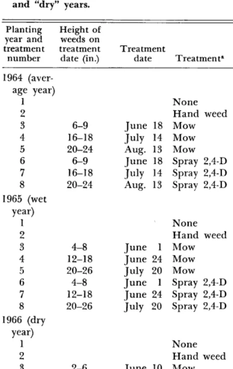
Table 1. Effects of weed control treatments on stand rat- ings of crested wheatgrass seedings in “average,” “wet,” and “dry” years.
Planting year and treatment number
1964 (aver- age year)
1 2 3 4 5 6 7 8 1965 (wet
year) 1 2 3 4 5 6 7 8 1966 (dry
year) 1 2 3 4 5 6 7 8
6-9 16-18 20-24 6-9 16-18 20-24
4-8 12-18 20-26 4-8 12-18 20-26
2-6 12 12 2-6 12 12
None 2.4
Hand weed 8.0
June 18 Mow 3.2
July 14 Mow 5.2
Aug. 13 Mow 3.8
June 18 Spray 2,4-D 7.4 July 14 Spray 2,4-D 3.2 Aug. 13 Spray 2,4-D 2.4
None 8.6
Hand weed 9.6
June 1 Mow 8.8
June 24 Mow 9.2 July 20 Mow 9.4 June 1 Spray 2,4-D 8.8 June 24 Spray 2,4-D 9.6 July 20 Spray 2,4-D 8.8
None .6
Hand weed 4.4
June 10 Mow .4
July 26 Mow .6
Aug. 30 Mow .8
June 10 Spray 2,4-D 1.0 July 26 Spray 2,4-D .4 Aug. 30 Spray 2,4-D .4
a Mowing was at a height of 1.5 inches, with the mowed vegeta- tion removed; an amine formulation of 2,4-D was applied at a rate of 3 lb/acre.
b Rating made in spring of year following planting. Rating of 0 = no stand; rating of 10 = perfect stand.
equals no seeded plants in the plot, and “10” equals the best stand the plot can be expected to support. In general, a rating of “6” or above is considered to be a satisfactory stand.
The spring of 1964 was slightly drier than “normal,” but it was still within the range of what can be called an “aver- age year.” However, the summer was particularly dry. Pre- cipitation in 1965 was slightly below normal in the early spring, but it was adequate for good germination of seeded grasses and weeds. June, with over 5 inches of rain, and July were wet. The winter of 1965-66 was dry, and 1966 was one of the driest years of record throughout the entire season.
Because of the wide differences in climatic conditions, it it was not possible to follow the study plan with regard to weed height at times of treatment. Weed heights at the time of treatment and dates of treatment are shown in Table 1.
Results and Discussion
Moderately dense stands of weeds developed on the plots in 1964 and 1965; in 1966 the weeds were sparse, scattered, and lacked vigor. The predomi- nant weeds were sunflowers (HeZianthus sp.), Rus- sian-thistle (Salsola kali var. tenuifolia Tausch), Belvedere summercypress (Kochia scoparia (I,.)
Schrad.), and prairie pepperweed (Lepidium densi- f lorum Schrad.).
The early spraying (weeds 6 to 12 inches high) was effective in all years because most weeds had emerged by that date; these plots remained almost free of weeds for the rest of the growing season. In 1964 and 1966, the weed reduction from 2,4-D on the 18- and 24-inch treatments was moderate to poor because of dry soil and poor growing condi- tions. In 1965, spraying killed weeds on both of the later treatment dates.
Early mowing (6 to 12 inch height) set the weeds back but did not kill many. The later mowing dates appeared much more harmful to the weeds, and, although many of the weeds were not killed, their growth was substantially retarded for the re- mainder of the season. No damage from mowing to the <grass seedlings was observed at any time.
In 1964, the most nearly “average” year of the three, the differences due to treatments were great- est (Table 1). Hand weeding produced an excel- lent stand. The early spraying eliminated the weeds before they could deplete the soil moisture supply, and a very good grass stand resulted. The other treatments (with the possible exception of mowing when weeds were 16 to 18 inches high) provided no worthwhile benefit as compared to no weed control.
The early moisture in 1965 was sufficient to give good seedling emergence, and the heavy June and July rains provided adequate moisture for both grass and weeds. Because of the abundance of moisture, weed control produced no benefit to grass stand establishment.
In the extreme drouth of 1966, no satisfactory stands were obtained. A fair stand was obtained by using hand weeding, but this varied greatly be- tween plots. Although early spraying killed weeds, the weeds had already depleted the limited mois- ture supply. Thus, in a year as dry as 1966, even the most intensive weed-control treatment did not produce a satisfactory stand, and the less intensive treatments resulted in failures. Furthermore, these poor grass stands were not a consequence of inade- quate germination and emergence, because good seedling stands of grass were observed in mid-May before the weeds depleted the soil moisture.
128 McGINNIES
stands and eliminated the weed problem because the weed seeds did not germinate at that season. However, at Fort Collins, satisfactory seedling stands from late summer plantings have not been obtained, but early spring plantings consistently produced good seedling emergence. The success of the spring plantings is not unexpected because, on the average, spring is the period of greatest pre- cipitation in this area.
Plummer et al. (1955) reported that Russian- thistle and other summer-growing annuals “make their growth after the grass seedlings are fairly well established, and so do not need to be eliminated.” In north-central Colorado, crested wheatgrass seed- lings will remain green and will continue growing throughout the summer of the seedling year, pro- vided sufficient moisture is available, rather than become dormant in midsummer as do the mature plants. Therefore, it would seem advisable to eliminate even the summer-growing weed species, so that more soil moisture will be available for the grass seedlings.
No evidence of damage to seedlings of crested wheatgrass, intermediate wheatgrass (Agropyror2.
intermedium (Host) Beauv.), pubescent wheat- grass (A. trichophorum (Link) Richt.), or Russian wildrye (EZymus junceus Fisch.) from mowing or from spraying with 2,4-D has been observed in the present study, or in other plantings at this location.
Although no seedling damage was observed from the heavy rate of application in this study, 3 lb/ acre of 2,4-D is generally considered to be an ex- cessive rate. However, determination of the most effective herbicide for local conditions or of opti- mum rates of application was beyond the scope of the present study. Further research is needed be- fore specific recommendations concerning herbi- cides and rate of application can be made.
The only serious problem encountered so far in using the weed-free seeding method described here has been with wind erosion which sometimes blows the seed out. Wind damage has been held to a minimum by using the strip-planting technique described by Bement et al. (1965). Establishment of stubble for erosion control (Hull et al, 1958) has been intentionally avoided, because the mois- ture that is needed to establish the cover crop which is to be cut for stubble would utilize soil moisture and thus defeat the purposes of the fal- lowing (Bement et al., 1965). Methods for con-
trolling wind erosion on clean seedbeds are being investigated. However, until better methods are developed, the strip-planting system should be used.
Where downy brome (Bromus tectorum L.) is present, most of its seed germinates in the fall or very early spring if sufficient moisture is available. The small amount of spring cultivation needed to smooth the seedbed has usually eliminated this very competitive weedy grass, at least for the re- mainder of that particular year.
Conclusions
If one is willing to accept the risk of a blow-out loss from wind, or if wind erosion can be con- trolled, then early spring planting on a clean, fal- lowed seedbed, followed by thorough weed control in the seedling stand, appears to offer the highest probability of successful grass establishment in north-central Colorado. Assuming that mechani- cal weeding is impractical on a range seeding, the broadleaf weeds can best be controlled with 2,4-D when they are still small, but spraying should be delayed until after most of the weed seeds have ger- minated. In average years, spraying will improve stands substantially because it will eliminate most of the weeds before they can deplete the soil mois- ture. If the soil moisture during the growing sea- son is more than adequate, there probably will not be any benefit from spraying, but no harm will have been done. If the year turns out to be excep- tionally dry, probably no treatment will produce a satisfactory stand, but this is one of the hazards of range seeding in semiarid zones where failures must be expected in some dry years in spite of good seeding techniques.
LITERATURE CITED
BEMENT, R. E., R. D. BARMINGTON, A. C. EVERSON, L. 0. HYLTON, JR., AND E. E. REMMENGA. 1965. Seeding of abandoned cropland in the central Great Plains. J. Range Manage. 18: 53-59.
HULL, A. C., JR., D. F. HERVEY, CLYDE W. DORAN, AND W. J. MCGINNIES. 1958. Seeding Colorado range lands. Colorado Exp. Sta. Bull. 498-S. 46 p.
MCGINNIES, WILLIAM J. 1966. Effects of shade on the sur- vival of crested wheatgrass seedlings. Crop Sci. 6:482-484. PLUMMER, A. PERRY, A. C. HULL, JR., GEORGE STEWART, AND
JOSEPH H. ROBERTSON. 1955. Seeding rangelands in Utah, Nevada, southern Idaho and western Wyoming.
and the Relation of Sulfur to
Other Nutrients as Diagnosed by
Plant Analysis’
LYNN 0. HYLTON,2 DONALD R. CORNELIUS, AND ALBERT ULRICH
Range Scientists, Crops Research Division, Agricultural Re- search Service, U.S.D.A., Berkeley, California; and Plant Physiologist, Department of Soils and Plant Nutrition, Uni-
versity of California, Berkeley, respectively.
Highlight
Sulfur needs of Spanish clover, Lotus purshianus (Benth.) Clements and Clements, were determined by plant analysis in a nutrient solution study. Top growth was affected more than root growth by changes in S supply. Protein synthesis in the shoots was affected little by S deficiency. Sulfate-S was better than organic-S or total-S to diagnose the S status of the plant adequately. The critical sulfate-S concentra- tion for growth of the plant is about 100 ppm, dry basis, in the middle stem section of the shoots.
Spanish clover is a native annual legume widely distributed in western United States. It is a key species in the management of the California range- land composed of an annual-plant mixture. Span- ish clover is important in the management of this unique rangeland because it is the only palatable plant that remains green and succulent in appreci- able amounts long after associated annuals have matured and diminished in feed value. Field tests (Green, 1959; Westfall, 1966) on soils of granitic origin have demonstrated that S fertilization will often lengthen the green period and increase total growth of Spanish clover.
The amount of S that legumes need, and when to apply S to prevent S deficiency, varies among species (Gilbert, 1951; Jordan and Ensminger,
1958). Symbiotic N fixation, soil characteristics, and climate, all influence the S needs of legumes (Walker, 1957). Sulfur requirements and esti- mated critical S concentrations have been reported for several introduced clovers (Jones, 1962; Jones and Martin, 1964) and for alfalfa (Pumphrey and Moore, 1965; Ulrich et al., 1967). But nothing is published about the concentration of S needed in Spanish clover to prevent S deficiency when other growth requirements are favorable. Guidelines are
1 Cooperative investigations of Crops Research Division, Agricultural Research Service, U.S. Department of Agri- culture, Berkeley, California; and the Department of Soils and Plant Nutrition, University of California, Berkeley. 2 Present address: San Joaquin Experimental Range, PSW
Forest Range Experiment Station, Coarsegold, California.
intrepret the data for a reliable diagnosis.
The purpose of this study is to provide basic in- formation about : 1) the effects of S supplied in nutrient solution on growth of Spanish clover, 2) the effects of S supply on certain nutrient concen- trations within plant tissues, 3) the combination of plant part and chemical form of S most sensitive for diagnostic purposes, 4) the critical S concentra- tion, and 5) how to interpret the results in terms of S needed to prevent S deficient plants.
Methods and Materials
Seeds of Spanish clover were germinated in flats of soil and allowed to grow until 3 trifoliate leaves had developed. On June 10, 1964, the seedlings were removed from the soil, the roots washed with tap water, and the seedlings transplanted to nutrient solutions in 20.liter tanks. No nodules were on the roots. Ten seedlings were supported on each tank and held individually in corks with non- absorbent cotton. Each tank contained 20 liters of an aer- ated nutrient solution made from reagent grade salts and distilled water. Mineral composition of the solutions at the time the seedlings were transplanted was: 7.5 N03-, 1.0 HzP04-, 4.0 Ca++, 4.0 K+ (plus K added with the variable S04’ treatments), 1.0 Mg”, 0.5 SiO,‘, and 0.5 Cl- (plus Cl added with certain micronutrients) in meq/liter; 0.25 B, 0.25 Mn, 0.025 Zn, 0.01 Cu, 0.005 MO, and 2.5 Fe in ppm. Iron was added as a FeCb-EDTA complex. Manganese, Zn, and Cu were added as chloride salts. Boron was added as HsBO, and MO as MoOa-2Hz0 (85% assay). Primary salts were Ca(N03)2-4Hz0, Mg(NO+-6H20, KNOS, KHZPOJ, KCl, and Na,SiO,-9H,O. A second addition of nutrients, equivalent to the foregoing, was made directly to the old solutions 21 days after transplanting. No nutrient solution was removed from the tanks except by plant growth. Dis- tilled water was added as needed to maintain about 20 liters of solution in each tank. The nutrient solutions were maintained between pH 6.0-7.0 with HCl. Sulfur was added as K,SO, at transplanting in the amounts shown in Tables 1 to 5, except for treatments 128 and 256 mg S/ plant, in which cases the first addition was limited to 64 mg S/plant. A second addition of 64 mg S/plant was made to the two highest S treatments 21 days after transplanting, and a final addition of 128 mg S/plant was made 7 days later to the highest S treatment. The S treatments were randomized in a serpentine, complete-block design with 5 replications. The plants were grown for 36 days in full greenhouse sunlight and carbon-filtered air.
130 HYLTON ET AL.
Table 1. Fresh weight, oven-dry weight, and number of shoots of Spanish clover as affected by S treatments.l
Change in
Oven-dry weight, total dry
Fresh wt g/plant wt in mg Top- root
Treatment, of tops, Tops+ per mg Number,
mg S/plant g/plant Tops Roots Roots change in S2 dry wt ratio, shoots/ plant
1.3 a” 0.24 a 0.24 a 0.48 a 1.0 a 4a
2,000
6.9 ab 1.25 b 1.23 b 2.48 b 1.1 ab 9b
1,070
13.3 b 2.12 c 1.43 bc 3.55 c 1.5 ab 10 bc
795
23.6 c 3.36 d 1.78 c 5.14 d 1.9b 11 cd
312
37.2 d 4.86 e 1.53 bc 6.39 d 3.6 c 11 cd
12
16 32
64
41.8 de 5.07 e 1.29 b 6.36 d 4.0 cd 12 d
67
45.7 e 5.40 e 1.23 b 6.63 d 4.3 cd 12d
9
47.2 e 5.60 e 1.18 b 6.78 d 4.8 d 12d
5
47.6 e 5.60 e 1.33 b 6.93 d 4.4 cd 12d
128 43.3 de 5.74 e 1.26 b 7.00 d 4.6 d 12d
256 45.6 e 5.52 e 1.15 b 6.67 d 4.8 d 12d
1 All data, except those in column 6, are means of 5 replications.
2 Values in column 6 show the unit change in total dry matter with each unit change in added S, calculated from means in column 5 and corresponding S treatments.
3 Values within a column followed by like letters are the same statistically. Duncan’s Multiple Range Test, 0.05 probability.
stems and the stems sectioned into upper, middle, and lower thirds. Top material not used for samples was weighed as residue. The roots were washed in distilled water and cen- trifuged at 40 g for 5 min.
All plant parts were dried in a forced-draft oven at 70 C. Dry weights of plant parts and residue were recorded. Total top weight was the sum of the weights for the plant parts plus the residue, but excluded roots. The dried material was ground to pass a 40.mesh sieve, or pulverized. Leaves 1 and 5 were not chemically analyzed.
Sulfate-S, total-S, nitrate-N, phosphate-P (P soluble in 2% acetic acid), and total-P were determined with respective methods described by Johnson and Ulrich (1959). Total-N was determined by a modified micro-Kjeldahl method to include nitrate-N (Humphries, 1956). Organic-S is reported as total-S minus sulfate-S and crude protein as organic-N times 6.25. Organic-N is total-N minus nitrate-N. After wet digestion wieh nitric and perchloric acids, Ca and Mg were determined by atomic absorption (Berry and Johnson, 1966), and K and Na by flame emission (Johnson and Ulrich, 1959).
Results and Discussion
Visual symptoms .-Plants grew equally well at all S treatments for 12 days after transplanting be- fore initial S deficiency symptoms appeared. Ter- minal leaflets of young leaves on S deficient plants became chlorotic before associated lateral leaflets or before leaflets of older leaves. A pinkish-red color, attributable to S deficiency, appeared along
the outer fringes of young leaflet blades. As S deficiency became more severe, the entire plant assumed a chlorotic appearance with a pinkish-red color on the margins of the leaflet blades and along the petiolules, petioles, and stems. Sulfur deficient plants were stunted and abnormally erect. They had small leaves and thin, brittle stems. Roots of S deficient plants were darker, fewer in number, but larger in diameter, than normal roots. No nodules were on the roots.
Table 2. Sulfate-S in various parts of Spanish clover as affected by S treatments.
Sulfate-S in ppm, dry basis1 Treatment,
mg S/plant 2
Leaves
3 4 6
Stem sections
Intact Fibrous Upper Middle Lower shoots roots
1 2 4 8 12 16 32 64 128 256
25 a2 35 ab
40 ab 50 b 13oc 200 c 380 d 600 e 510 de 590 e
20 a 30 ab 40 b 65 c 100d
120d 330 e 570 f 500 f 540 f
25 a 20 a 40 b 65 c 75 cd 95 d 380 e 550 f 530 f 600 f
30 a 35 ab 45 b 70 c 95 c 170d 440 e 550 ef 530 ef 650 f
30 a 30 a 45 a 45 a 140b 260 c 1,610 d 2,160 d 1,960 d 1,970 d
30 a 20 a 20 a 40 a 210b 610 c 2,820 d 3,040 d 2,890 d 2,870 d
45 a 40 a 60 a 140b 800 c 1,390 d 2,750 e 2,630 e 2,590 e 2,520 e
30 a 55 a 85 ab 100b 270 c 510d 1,310 e 1,460 e 1,530 e 1,420 e
80 a 70 a 85 a 420 b 410b 1,430 c 5,170 d 7,260 d 8,910 d 6,630 d
1 Data are means of 5 replications.
2 Values within a column followed by like letters are the same statistically, when determined on the logs of these data. Duncan’s Multiple Range Test, 0.05 probability.
when plants were severely deficient in S, 1 mg of added S produced about 1 g of dry plant material. Efficiency of S utilization by the plant decreased as the S needs of the plant were met.
Number of shoots per plant increased only about 22% with an &fold increase in S supply, from 1 to 8 mg S/plant (Table l), while top yield, dry basis, increased 290%. Top yield was clearly influenced more by size of leaves, stems, and shoots, than by number of shoots.
Sulfate-S in plant parts.-Sulfate-S in the plant varied greatly with the plant part and the S treat- ment (Table 2). Less variation occurred in sul- fate-S concentration among plant parts at low S treatments (less than 8 mg S/plant) than at ade- quate and high S treatments. Roots had the widest range in sulfate-S concentration, from low to high, followed by the middle stem section. Leaf-blade tissue had the narrowest range in sulfate-S concen-
tration, regardless of leaf age. At high S treatments (64 mg S/plant or more) only about 20% as much sulfate-S accumulated in leaf-blade tissue as in the adjacent stem tissue (Table 2). These observations are in agreement with findings for subterranean clover (Jones, 1962) but are in contrast to those found for alfalfa (Ulrich et al., 1967). The latter workers found much higher accumulations of sul- fate-S in leaf blades than in stems of alfalfa with ample S in solution. They also found that within the stems of alfalfa, the upper stem sections con- tained more sulfate-S than the middle and lower stem sections. Distribution of sulfate-S within the stem of Spanish clover, from treatments of 32 mg S/plant and more, was as follows: middle third > lower third > upper third (Table 2). Sulfate-S concentration was consistently higher in the lower third of the stem than in the middle third and up- per third, with 16 mg S/plant and less in solution.
Table 3. Sulfate-S, organic-S, and total-S in the middle stem section and in the intact shoot of Spanish clover as af- fected by S treatments.
Sulfur concentrations in %, dry basis’
Treatment, mg S/plant
1 2 4 8 12 16 32 64 128 256
Middle stem section Shoot
Sulfate Organic Total Sulfate Organic Total
-2 a” 0.02 a 0.02 a _2 aY 0.03 a 0.03 a
-’ a 0.02 a 0.02 a _2 a 0.05 ab 0.05 a
-’ a 0.03 ab 0.03 a -’ a 0.06 b 0.06 a
-’ a 0.04 b 0.04 ab _2 a 0.10 c 0.10 b
0.02 ab 0.06 c 0.08 bc 0.02 ab 0.15 de 0.17 c 0.06 b 0.07 c 0.13 c 0.05 b 0.14 d 0.19 c 0.28 c 0.09 d 0.37 d 0.13 c 0.15 de 0.28 d 0.30 c 0.09 d 0.39 d 0.14 c 0.17 ef 0.31 de 0.29 c 0.08 d 0.37 d 0.15 c 0.16 def 0.31 de 0.29 c 0.08 d 0.37 d 0.14 c 0.18 f 0.32 e
1 Data are means of 5 replications. 2 Less than 0.01%.
6
HYLTON ET AL.
Sulfate-S
in middle stem section (ppm)
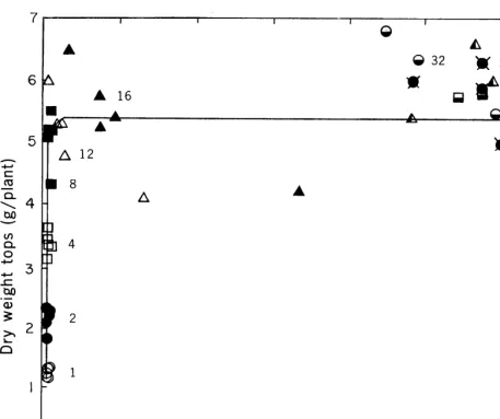
FIG. 1. Relation of dry weight of tops to sulfate-S in the middle stem section of Spanish clover grown from nutrient solutions. Numbers with 5 like symbols show the mg of S per plant for each of ten S treatments. The critical sulfate-S concentration is 100 ppm of sulfate-S in the middle stem section, dry basis. This value was taken from the curve at a 5% reduction from average maximum top growth.
There was no measurable difference in concentra- tion of sulfate-S in leaf-blade tissue attributable to leaf age. This was true even at low S treatments where visual S deficiency symptoms appeared first and were more pronounced in the young leaves. Evidently the transfer of sulfate-S or elaborated-S from older to younger leaves was not sufficiently rapid, if at all, to prevent the yellowing observed first in young leaflets.
Organic-S and total-S in the plant.---Most of the S in plants that were under stress for S was in the organic form; i.e., from treatments of less than 8 mg S/plant (Tables 1 and 3). This remained true for S in the shoots even with ample S in solution. Apparently the organic-S concentration in the shoots was influenced more by organic-S in the leaf blades than by organic-S in the stems. Sulfur values in Table 3 for the middle stem section show that organic-S increased very little, relative to sul-
fate-S in this plant part, when S in solution was adequate to high; i.e., 32 mg S/plant or more.
FIG. 2a. tions. FIG. 2b.
Leaf 4
6
500
1000
0
500
Sulfate-S
(ppm)
Relation of dry weight of tops to sulfate-S in leaf blades 4 and 6, dry basis, of Spanish clover grown from nutrient solu- Refer to Fig. 1 for identification of symbols.
Intact shoot from a normal plant of Spanish clover. Numbers 1 to 6 show immature to matured leaves, respectively. Stem sections were obtained by sectioning the stem into thirds after leaves were removed.
crude protein content, in the shoot changed little with changes in S treatment. Crude protein ap- pears to have increased in the middle stem section of S-deficient plants but this increase may have been caused by amino acids and amides rather than protein. Corresponding increases did not occur in leaf blades. Nitrate-N did not accumulate in S deficient plants. These data suggest, therefore, that protein synthesis in the shoot was affected little by S deficiency. Crude protein would be expected to have a smaller percentage of S containing amino acids in S deficient plants than in normal plants, even though the total content of crude protein is the same.
Cation concentrations in the plant as affected by S supply are shown in Table 5. Calcium and Mg concentrations were higher in the shoot than in the middle stem section, regardless of the S treatment. Undoubtedly, much of this difference was from the contribution made to the shoot by the leaves and leaf buds where nucleoproteins, chlorophyll, and, in normal plants, new cell walls were being formed.
Potassium concentration increased more in the middle stem section than in the shoot with cor- responding increases in KzS04 additions (Table 5).
Plant growth in relation to sulfur in plant parts.-
Fig. 1 and 2a show detailed calibration graphs for the middle stem section and for leaves 4 and 6, re- spectively. These graphs were obtained by plotting dry weight of tops against the sulfate-S concentra- tion in the respective plant parts. The much greater accumulation of sulfate-S in the middle stem section, primarily conductive tissue, than in adjacent leaf blades, primarily photosynthetic tis- sue, is illustrated (Fig. 1, 2a, and 2b). This differ- ence existed only for plants supplied with 12 mg of S/plant or more. Graphs for the upper and lower stem sections and for the intact shoot were similar to Fig. 1, except for differences in sulfate-S accu- mulation with high S treatments as shown in Ta- ble 3. Likewise, graphs for leaves 2 and 3 were similar to Fig. 2a.
134 HYLTON ET AL.
Table 4. Phosphorus, nitrogen, and crude protein in the middle stem section and in the shoot of Spanish clover as affected by S treatments.
Concentrations in %, dry basis’
Middle stem section Shoot
Treatment, Phosphate Total Nitrate Total Crude Phosphate Total Nitrate Total Crude
mg S/plant P P N N Protein” P P N N Protein2
1 0.29 a3 0.34 a 0.06 a 2 0.32 ab 0.36 ab 0.17 b 4 0.33 ab 0.37 ab 0.36 c 8 0.31 ab 0.38 ab 0.78 d 12 0.35 bc 0.42 bc 1.03 ef 16 0.40 cd 0.48 cd 1.09 f 32 0.44 d 0.52 d 0.97 e 64 0.44 d 0.53 d 0.93 e 128 0.43 d 0.52 d 0.95 e 256 0.42 d 0.52 d 0.97 e
4.44 d 27.4 4.14 d 24.8 3.60 c 20.2 2.67 b 11.8 2.36 a 8.3 2.51 ab 8.9 2.39 a 8.9 2.36 a 8.9 2.34 a 8.7 2.38 a 8.8
0.45 de 0.51 cde 0.11 a 4.16 ab 25.3 0.37 ab 0.42 ab 0.18 a 4.07 a 24.3 0.34 a 0.41 a 0.32 b 4.05 a 23.3 0.34 a 0.42 ab 0.58 c 4.02 a 21.5 0.40 bc 0.46 bc 0.74 d 4.32 abc 22.4 0.42 cd 0.49 cd 0.86 d 4.51 bed 22.8 0.48 e 0.54 de 0.82 d 4.73 d 24.4 0.49 e 0.55 e 0.75 d 4.65 cd 24.4 0.47 e 0.54 de 0.84 d 4.75 d 24.4 0.48 e 0.55 e 0.80 d 4.76 d 24.7
l Data are means of 5 replications.
2 “Crude protein” is organic-N times 6.25; organic-N is total-N minus nitrate-N.
3 Values within a column followed by like letters are the same statistically. Duncan’s Multiple Range Test, 0.05 probability.
increased with additions of 1, 2, 4, and 8 mg S,/ plant, respectively, but there was no significant change in sulfate-S concentration in the middle stem section with these S treatments (Fig. 1). With S additions above 12 mg S/plant, however, concen- trations of sulfate-S in the middle stem increased rather rapidly with no corresponding increase in top growth.
Figure 3 and 4 show schematically the relation of top growth to sulfate-S, organic-S, and total-S in the middle stem section and in the shoot, respec- tively. Sulfate-S values for both plant parts changed little until the S needs of the plant were nearly met. When top growth approached a maxi- mum, sulfate-S concentrations increased rapidly. Organic-S, in contrast, increased 3-fold in the shoot
before the S needs of the plant were fully met (Fig. 4). Likewise, total-S increased gradually in the shoot with increased top growth. Total-S in the middle stem section and in the shoot of S deficient plants was influenced primarily by changes in or- ganic-S (Fig. 3 and 4). But total-S in the middle stem section of normal plants was influenced more by changes in sulfate-S than by changes in organic- S (Fig. 3). Total-S in shoots from normal plants was influenced about equally by sulfate-S and organic-S.
Critical S concentration and interpretation.-A
reliable diagnosis of the nutrient status of plants depends upon a knowledgeable interpretation of the sample data. The calibration graph in Fig. 1 illustrates the best plant part and best chemical
Table 5. Cation concentration in the middle stem section and in the shoot of Spanish clover as affected by S treatments.
Concentrations in %, dry basis’-
Treatment, Middle stem section Shoot
mg S/plant Ca Mg K Na Ca Mg K Na
8
12 16 32 64 128 256
0.51 a” 0.12 d 1.73 a -3 a 2.33 d 0.62 ab 0.10 bc 2.76 b -3 a 2.63 e 0.66 b 0.08 a 3.27 c 0.03 b 2.38 d 0.69 b 0.08 a 4.23 d 0.04 bc 2.12 c 0.84 c 0.1 I cd 5.18 e 0.04 bc 2.03 bc 0.72 b 0.12 d 5.54 ef 0.05 c 2.08 c 0.69 b 0.12 d 5.51 ef 0.05 c 2.01 bc 0.69 b 0.12 d 5.69 f 0.05 c 1.99 bc 0.62 ab 0.11 cd 5.81 fg 0.05 c 1.85 ab 0.63 ab 0.10 bc 6.20 g 0.04 bc 1.74 a
0.40 b 2.13 a -3 a 0.38 b 2.35 a -3 a 0.32 a 2.67 b 0.01 ab 0.28 a 3.07 c 0.02 bc 0.31 a 3.43 d 0.03 c 0.31 a 3.61 de 0.03 c 0.31 a 3.67 e 0.03 c 0.32 a 3.74 ef 0.03 c 0.31 a 3.93 fg 0.03 c 0.29 a 4.15 g 0.03 c
1 Data are means of 5 replications.
2 Values within a column followed by like letters are the same statistically.