Decoding Random Binary Linear Codes in
2
n/20: How
1 + 1 = 0
Improves Information Set Decoding
Anja Becker1, Antoine Joux1,2, Alexander May3!, and Alexander Meurer3!!
1 Universit´e de Versailles Saint-Quentin, Laboratoire PRISM 2 DGA
3 Ruhr-University Bochum, Horst G¨ortz Institute for IT-Security
[email protected],[email protected]
{alex.may,alexander.meurer}@rub.de
Abstract. Decoding random linear codes is a well studied problem with many applications in complexity theory and cryptography. The security of almost all coding and LPN/LWE-based schemes relies on the assumption that it is hard to decode random linear codes. Recently, there has been progress in improving the running time of the best decoding algorithms for binary random codes. The ball collision technique of Bernstein, Lange and Peters lowered the complexity of Stern’s information set decoding algorithm to20.0556n. Usingrepresentations this bound was improved to20.0537nby May, Meurer and Thomae. We show how to further increase the number of representations and propose a new information set decoding algorithm with running time20.0494n.
1 Introduction
The NP-hard problem of decoding a random linear code is one of the most promising problems for the design of cryptosystems that are secure even in the presence of quantum computers. Almost all code-based cryptosystems, e.g. McEliece, rely on the fact that random linear codes are hard to decode. In or-der to embed a trapdoor in coding-based cryptography one usually starts with a well-structured secret codeCand linearly transforms it into a codeC! that is supposed to be indistinguishable from a random code.
An attacker has two options. Either he tries to distinguish the scrambled version C! of C from a random code by revealing the underlying structure, see [10, 27]. Or he directly tries to run a generic decoding algorithm on the scrambled codeC!.
Also closely related to random linear codes is the learning parity with noise (LPN) problem that is frequently used in cryptography [1, 13, 16]. In LPN, one directly starts with a random linear code C and the LPN search problem is a decoding problem in C. It was shown in [26] that the popular LPN decision
variant, a very useful tool for many cryptographic constructions, is equivalent to the LPN search problem, and thus equivalent to decoding a random linear code. The LWE problem of Regev [26] is a generalization of LPN to codes over a largerfield. Our decoding algorithm could be adjusted to work for these largerfields (similar to what was done in [8, 25]). Since the decoding problem lies at the the heart of coding-based and LPN/LWE-based cryptography it is necessary to study its complexity in order to define proper security parameters for cryptographic constructions.
Let us start by providing some useful notation. A binary linear codeC is a k-dimensional subspace of Fn2 wherenis called the length of the code and R := nk is called its rate. A random k-dimensional linear codeC of length n can be defined as the kernel of a random full-rank matrixH∈R F(2n−k)×n, i.e.
C = {c ∈ Fn2 | Hct = 0t}. The matrixHis called a parity check matrix of C. For ease of presentation, we use the convention that all vectors are column vectors which allows as to omit all transpositions of vectors.
The distancedof a linear code is defined by the minimal Hamming distance between two codewords. Hence every vector xwhose distance to the closest codeword c ∈ C is at most the error correction capacity ω = "d−1
2 # can be uniquely decoded toc.
For any pointx=c+e∈Fn
2that differs from a codewordc∈Cby an error vectore, we define itssyndromeass(x) := Hx = H(c+e) = He. Hence, the syndrome only depends on the error vectore and not on the codewordc. Thesyndrome decoding problemis to recoverefroms(x). This is equivalent to decoding inC, since the knowledge ofesuffices to recovercfromx.
Usually in cryptographic settings the Hamming weight ofeis smaller than the error correction capability, i.e.wt(e) ≤ω ="d−21#, which ensures unique decoding. This setting is also known as half/bounded distance decoding. All known half distance decoding algorithms achieve their worst case behavior for the choicewt(e) =ω. As a consequence we assumewt(e) =ωthroughout this work. In complexity theory, one also studies the so-calledfull decoding where one has to compute a closest codeword to a givenarbitraryvectorx∈Fn
2. We also give the complexity of our algorithm for full decoding, but in the following we will focus on half-distance decoding.
coefficientF(R)as defined in [8], i.e.F(R) = limn→∞1nlogT(n, R)which suppresses polynomial factors since limn1logp(n) = 0 for any polynomial p(n). Thus, we have T(n, R) = 2nF(R)+o(n) ≤ 2n&F(R)'ρ for large enough n. We obtain the worst-case complexity by taking max0<R<1&F(R)'ρ. Here, &x'ρ := &x·10ρ' ·10−ρdenotes rounding up x ∈ Rto a certain number of
ρ∈Ndecimal places.
Related work.In syndrome decoding one has to computeefroms(x), which means that one has tofind a weight-ωlinear combination of the columns ofH that sums to the syndromes(x)overFn2−k. Thus, a brute-force algorithm would require to compute!nω" column sums. Inspired by the work of Prange [24], it was already mentioned in the original work of McEliece [21] and later more carefully studied by Lee and Brickell [18] that the following approach, called
information set decoding, yields better complexity.
Information set decoding basically proceeds in two steps, an initial trans-formation step and a search step. Both steps are iterated in a loop until the al-gorithm succeeds. The initial transformation step starts by randomly permuting the columns ofH. In particular, this permutes theωcolumns ofHthat sum to s(x), and thus permutes the coordinates ofe. Then we apply Gaussian elimina-tion on the rows ofHin order to obtain a systematic form(Q | In−k), where Q∈F(n−k)×k
2 andIn−kis the(n−k)-dimensional identity matrix. The
Gaus-sian elimination operations are also applied tos(x)which results in˜s(x). Let usfix an integerp < ω. In the search step, we compute for every linear combination ofpcolumns fromQits Hamming distance tos˜(x). If the distance is exactly ω−p then can we add to our p columns those ω −p unit vectors fromIn−kthat exactly yields˜(x). Undoing the Gauss elimination recovers the
desired error vectore. Obviously, information set decoding can only succeed if the initial column permutation results in a permutedethat has exactlypones in itsfirstkcoordinates andω−pones in its lastn−kcoordinates. Optimization ofpleads to a running time of20.05752n.
Leon[19] and Stern[29] observed in 1989 that one can improve on the run-ning time when replacing in the search step the brute-force search for weight-p linear combinations by a Meet-in-the-middle approach. Let us fix an integer # <n −kand let us project(Q |In−k)to itsfirst#rows. We split the projec-tion ofQinto two matricesQ1,Q2each havingk2 columns. Then we create two lists L1,L2 that contain all weight-p2 linear combinations of columns fromQ1 andQ2, respectively. Moreover, we add the projection of˜s(x)to every element inL2and sort the resulting list.
co-ordinates. As before, if the remaining coordinates differ froms˜(x)by a
weight-(ω−p)vector, then we can correct these positions by suitable unit vectors from
In−k. The running time of this algorithm is20.05564n.
The ball collision technique of Bernstein, Lange and Peters [4] lowers this complexity to20.05559n by allowing a non-exact matching of the elements of L1 and L2. The same asymptotic complexity can be achieved by transform-ingHinto (Q | I 0
n−k−#)withQ ∈ F
(n−k)×(k+$)
2 , as proposed by Finiasz and Sendrier [11]. The listsL1,L2 then each contain all weight-p2 sums out of k+2$ columns. The asymptotic analysis of this variant can be found in [22].
Notice thatfinding a weight-p sum of columns ofQ that exactly matches
˜
s(x) in #coordinates is a vectorial version of the subset sum problem in F$2. This vectorial version was called the column match problemby May, Meurer and Thomae (MMT) [22], who adapted the subset sum representation technique from Howgrave-Graham and Joux [14] to the column match problem.
LetQ∈F2(n−k)×(k+$)be as before, whereq1, . . . ,qk+$denote the columns
of Q. A Meet-in-the-Middle approach matches the first # coordinates via the
identity #
i∈I1 qi =
#
i∈I2
qi+ ˜s(x) , (1)
whereI1 ⊂$1,k+2$%,I2 ⊂$k+2$+ 1, k+#%and|I1|=|I2|= p2.
Using the representation technique, one choosesI1 andI2 no longer from half-sized intervals but they both are chosen from the whole interval[1, k+#] such that I1 ∩I2 = ∅. Thus, every solution I admits!p/p2" representations I = I1 ∪I2. Notice that increasing the range of I1, I2 also increases the size of the listsL1andL2 from
!(k+$)/2
p/2
"
to!kp/+2$". But constructing only a!p/p2"−1 -fraction of each list suffices to let a single representation of the solution sur-vive on expectation. This approach leads to an algorithm which runs in time
20.05364n.
Our contribution.We propose to choose|I1|=|I2|= p2 +εfor some ε >0 such that|I1∩I2|=ε. So we allow forεcolumnsqi that appear on both sides
of identity (1). Thus every solution I is written as the symmetric difference I = I1∆I2 := I1∪I2\(I1 ∩I2), where we cancel out all εelements in the intersection ofI1 andI2.
that every of thepelements inI =I1∪I2can appear either as an element ofI1 or as an element ofI2, so it can appear on both sides of identity (1).
In contrast, we choose fully intersecting setsI1, I2 and additionally allow for a union of intersecting sets. Thus, we additionally allow that even those k+#−pelements that areoutside ofI =I1∪I2 may appear inI1, I2as long as they appear in both sets, and thus cancel out. This drastically increases the number of representations, since for random code instances the number of zeros in an error vectoreis much larger than the number of ones. Whereas MMT only allow to split each 1-entry ofeinto two parts, either1 = 0 + 1or1 = 1 + 0, we also allow to split each 0-entry ofeinto two parts, either0 = 0+0or0 = 1+1. Hence our benefit comes from using the equation1 + 1 = 0inF2. Notice that our approach therefore increases the number of representation per solutionI to
! p
p/2
"
·!k+%$−p
"
.
Our main algorithmic task that we describe in this work is the construction of two lists L1,L2 such that a single representation of each solution survives. This is realized by a three-level divide-and-conquer algorithm that is similar to Wagner’s generalized birthday algorithm [30].
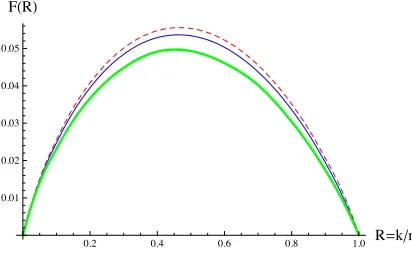
Our enhanced representation technique allows us to significantly lower the asymptotic running time to20.04934n. The followingfigure shows the curve of
the complexity coefficient for the two most recent algorithms [4, 22] compared to our new algorithm.
0.2 0.4 0.6 0.8 1.0 R!k!n 0.01
0.02 0.03 0.04 0.05
F"R#
Fig. 1: Comparison ofF(R)for code rates 0 < R < 1for bounded distance decoding. Our algorithm is represented by the thick curve, MMT is the thin curve and Ball-collision is the dashed curve.
2 Generalized Information Set Decoding
Re-call that the input to an ISD algorithm is a tuple(H,s)whereH ∈ F(2n−k)×n is a parity check matrix of a random linear [n, k, d]-code and s = He is the syndrome of the unknown error vectoreof weightω := wt(e) ="d−21#.
ISD is a randomized Las Vegas type algorithm that iterates two steps until the solution eis found. The first step is an initial linear transformation of the parity check matrixH, followed by a search phase as the second step.
In the initial transformation, we permute the columns of H by multiply-ing with a random permutation matrix P ∈ Fn×n
2 . Then we perform Gaus-sian elimination on the rows ofHP by multiplying with an invertible matrix
T ∈ F2(n−k)×(n−k). This yields a parity check matrixH˜ = THPin quasi-systematic form containing a0-submatrix in the right upper corner as illustrated in Fig. 2. Here we denote byQI the projection ofQto the rows defined by the
index set I ⊂ {1, . . . , n−k}. Analogously, we denote by QI the projection
ofQto its columns. In particular we define[#] := {1, . . . , #}and[#, n−k] =
{#, . . . , n−k}. We denote the initial transformation Init(H) :=THP.
˜
H
=
0
z k}|+! {z n−}|k−! { z
}|
{ !
z
}|
{
n−k−!
| {z }
p ω| {z }−p
Q
[#]I
n−k−#Q
[#+1,n−k]Fig. 2: Parity check matrixH˜ in quasi-systematic form.
We set˜s := Tsand look for an ISD-solutione˜of( ˜H,˜s), i.e. we look for an
˜
esatisfyingH˜˜e = ˜sand wt(˜e) = ω. This yields a solution e = P˜efor the original problem. Notice that applying the permutation matrix to˜eleaves the weight unchanged, i.e.wt(e) =ω, andTHe= ˜He˜= ˜s=TsimpliesHe=s as desired. In the search phase, we try to find all error vectors˜e that have a specific weight distribution, i.e. we search for vectors that can be decomposed intoe˜ = (˜e1,˜e2) ∈Fk2+$×F2n−k−$wherewt(˜e1) =pandwt(˜e2) = ω−p. SincePshufflese’s coordinates into random positions,˜ehas the above weight distribution with probability
P =
!k+l
p
"!n−k−l
ω−p
" !n
ω
The inverse probability P−1 is the expected number of repetitions until˜ehas the desired distribution. Then it suffices tofind the truncated vector˜e1 ∈Fk2+$ that represents the position of the firstp ones. To recover the full error vector
˜
e = (˜e1,˜e2), the missing coordinatese˜2 are obtained as the last n−k −# coordinates ofQ˜e1+ ˜s. Hence, the goal in the ISD search phase is to compute the truncated error vector˜e1 efficiently. For the computation ofe˜1we focus on the submatrix Q[$] ∈ F2$×(k+$). Since we fixed the 0-submatrix in the right-hand part of H˜, we ensure that Q˜e1 exactly matches the syndrome˜s on its
first#coordinates. Finding an˜e1with such a property was called thesubmatrix
matching problemin [22].
Definition 1 (Submatrix Matching Problem).Given a random matrixQ ∈R F$2×(k+$) and a target vector s ∈ F$2, the submatrix matching problem (SMP)
consists in finding a set I of size psuch that the corresponding columns of Q sum up tos, i.e. tofindI ⊆[1, k+#],|I|=psuch that
σ(QI) :=#
i∈I
qi =s, whereqi is thei-th column ofQ.
Note that the SMP itself can be seen as just another syndrome decoding instance with parity check matrixQ, syndromes∈F$
2and parameters[k+#, #, p]. Our improvement stems from a new algorithm COLUMNMATCH allowing to solve the SMP more efficiently by using more representations of a solutionI. In Alg. 1 we describe the resulting ISD algorithm. Here we denote for a vector
x ∈ Fn2 and an index set I ⊂ [n] by xI ∈ F|2I| the restriction of x to the coordinates ofI.
Algorithm 1GENERALIZEDISD
Input:Parity check matrixH∈F(n−k)×n
2 , syndromes=Hewithwt(e) =ω.
Output: Errore∈Fn
2
Parameters:p,!
Repeat
ComputeH˜ ←Init(H)ands˜←TswhereH˜ =THP,Prandom permutation. ComputeL=COLUMNMATCH(Q[#],˜s
[#], p).
For allsolutions˜e1 ∈ Ldo
Ifwt(Q˜e1+ ˜s) =ω−pthen
Computeee←(˜e1,e˜2)∈Fn2 wheree˜2←(Q˜e1+ ˜s)[#+1,n−k]
Outpute=eeP.
3 The Merge-Join Building Block
In order to realize our improved SMP algorithm, wefirst introduce an essential building block that realizes the following task. Given a matrixQ∈F$2×(k+$)and two listsL1andL2containing binary vectorsx1, . . . ,x|L1|andy1, . . . ,y|L2|of
lengthk+#, we aim to join those elementsxi andyj into a new listL=L1'(
L2whose sum has weightp, i.e.wt(xi+yj) =p. Furthermore, we require that
the corresponding column-sum ofQalready matches a given target t ∈Fr
2 on its right-mostr≤#coordinates, i.e.(Q(xi+yj))[r]=t.
L1
010100
i0→
110100
i1→100100
L2
011100←j0 ←j1
110100
r #$
L
! !000
! !000
! !000
! !000
Fig. 3: Illustration of the MERGE-JOINalgorithm to obtainL=L1#$L2.
Searching for matching vectors (Qyj)[r] +t and (Qxi)[r] accomplishes this task. We call all matching vectors with weight different frompinconsistent so-lutions. Notice that we might also obtain the same vector sum from two different pairs of vectors from L1,L2. In this case we obtain a matched vector that we already have, which we call aduplicate. During our matching process wefilter out all inconsistent solutions and duplicates.
The matching process is illustrated in Fig. 3. The complete algorithm is given as Alg. 2 and is based on a classical algorithm from Knuth [17] which realizes the collision search as follows. Sort thefirst list lexicographically ac-cording to ther-bit labelsL1(xi) := (Qxi)[r]and the second list according to the labelsL2(yj) := (Qyj)[r]+t. We addtto the labels of the second list to guarantee(Q(xi+yj))[r]=t.
To detect all collisions, one now initializes two counters i and j starting at the beginning of the lists L1 andL2 and pointing at elementsxi andyj. As
long as those elements do not yield a collision, either ior j is increased de-pending on the relative order of the labelsL1(xi)andL2(yj). Once a collision L1(xi) =L2(yj)occurs, four auxiliary countersi0, i1andj0, j1are initialized withiandj, respectively. Theni1 andj1 can further be incremented as long as the list elements retain the same labels, whilei0 andj0 mark thefirst collision
Algorithm 2MERGE-JOIN
Input:L1,L2, r, pandt∈Fr
2
Output:L=L1#$L2
Lexicographically sort L1 and L2 according to the labels L1(xi) := (Qxi)[r] and L2(yj) := (Qyj)[r]+t.
Set collision counterC←0. Leti←0andj←(|L2| −1)
Whilei <|L1|andj <|L2|do
IfL1(xi)<lexL2(yj)theni+ +
IfL1(xi)>lexL2(yj)thenj+ +
IfL1(xi) =L2(yj)then Leti0, i1←iandj0, j1←j
Whilei1<|L1|andL1(xi1) =L1(xi0)doi1+ +
Whilej1<|L2|andL2(yj1) =L2(yj0)doj1+ +
Fori←i0toi1−1do Forj←j0toj1−1do
C=C+ 1
Insert collisionxi+yjinto listL(unlessfiltered out) Leti←i1, j←j1
OutputL, C.
setsC1 ={xi0, . . . ,xi1}andC2 ={yj0, . . . ,yj1}such that all possible
com-binations yield a collision, i.e. the setC1 ×C2 can be added to the output list
L.
This procedure is then continued withi ← i1 andj ← j1 until one of the countersi, jarrives at the end of a list. As mentioned before, we remove on the
fly inconsistent solutions with incorrect weightwt(xi+yj)/=pand duplicate
elementsxi+yj =xk+y$.
Note that we introduced a collision counterC which allows us to take into account the time that is spent for removing inconsistent solutions and duplicates. The total running time ofMERGE-JOINis given by
T = ˜O(max{|L1|,|L2|, C}) .
Assuming uniformly distributed labelsL1(xj)andL2(yj)it holds thatE[C] = |L1| · |L2| ·2−r.
4 Our New Algorithm for Solving the Submatrix Matching Problem
As explained in Section 2, improving the submatrix matching problem (SMP) automatically improves information set decoding (ISD).
In the MMT algorithm [22] a weight-perror vectore∈ Fk2+$is written as the sume1 +e2. However, MMT only allow that every 1-entry splits to either a 1-entry inx1 and a 0-entry inx2, or vice versa. Ifwt(e1) = wt(e2) = p2 this allows for!p/p2"different representations as a sum of two vectors.
Our key observation is that we can also split the0-entries ofeinto either
(0,0) or(1,1). Hence if we choosewt(e1) = wt(e2) = p2 +εthen we gain a factor of!k+ε$−p", namely the number of positions where we split as (1,1). Notice that in all coding-based scenarios wt(e) is relatively small compared
tokandn. Thusecontains many more zeros than ones, from which our new
representation heavily profits.
To solve the SMP, we proceed as follows. LetI ⊂[k+#]be the index set of cardinalitypwithσ(QI) =sthat we want tofind.
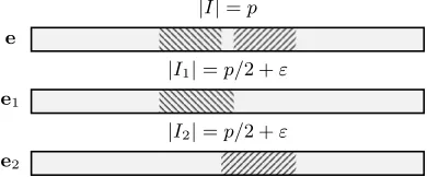
We representI by two index setsI1andI2of cardinalityp2+εcontained in the whole interval[k+l]and requireI1andI2 to intersect in afixed number of εcoordinates as illustrated in Fig. 4.
|I|=p
e
|I1|=p/2 +ε
e1
|I2|=p/2 +ε
e2
Fig. 4: Decomposition of an index setIinto two overlapping index sets.
The resulting index setIis then represented as the symmetric differenceI1∆I2 :=
(I1∪I2)\(I1∩I2)which yields an index setI of cardinality pas long asI1 andI2intersect in exactlyεpositions.
It turns out that the optimal running time can be obtained by applying the representation technique twice, i.e. we introduce further representations of the index setsI1andI2 on a second computation layer.
4.1 OurCOLUMNMATCHAlgorithm
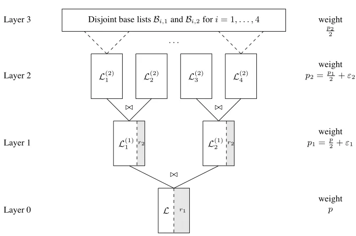
Our algorithm can be described as a computation tree of depth three, see Fig. 7 for an illustration. We enumerate the layers from bottom to top, i.e. the third layer identifies the initial computation of disjoint base lists B1 andB2 and the zero layer identifies thefinal output listL.
Recall that we aim tofind an index setI of sizep with&i∈Iqi = s. We
. . .
Disjoint base listsBi,1andBi,2fori= 1, . . . ,4
Layer 3
Layer 2
Layer 1
Layer 0
weight p2
2
weight
p2= p1
2 +ε2
weight
p1= p2+ε1
weight
p
#$ #$
#$
r2 r2
r1 L
L(1)1 L
(1) 2 L(2)1 L
(2)
2 L
(2)
3 L
(2) 4
Fig. 5: Illustration of the COLUMNMATCHalgorithm.
allow on the first and second layer, respectively. In the following description, we equip every object with an upper index that indicates its computation layer, e.g. a listL(2)j is contained in the second layer.
On thefirst layer, we search for index setsI1(1) andI2(1) in[k+#]of size p1 := p2+ε1which intersect in exactlyε1coordinates such thatI =I1(1)∆I
(1) 2 . In other words, we create lists of binary vectorse(1)1 ande(1)2 of weightp1and search for tuples(e(1)1 ,e(1)2 )such thatwt(e(1)1 +e(1)2 ) =pandQ(e(1)1 +e(1)2 ) =
s.
Note that the number of tuples(e(1)1 ,e(1)2 )that represent a single solution vector
eis
R1(p, #;ε1) :=
'
p
p
2
('
k+l−p
ε1
(
. (3)
More precisely, the algorithm proceeds as follows. Wefirst fix a random vectort(1)1 ∈RFr12 , sett
(1)
2 :=s[r1]+t(1)2 and compute two lists
Li(1)={ei(1) ∈F2k+$ | wt(ei) =p1and(Qe(1)i )[r1]=t(1)i }fori= 1,2.
Observe that any two elements e(1)i ∈ L(1)i , i = 1,2, already fulfill by
con-struction the equation (Q(e(1)1 +e2(1)))[r1] = s[r1], i.e. they already match the syndromes onr1 coordinates. In order to solve the SMP, we are interested in a solution e= e(1)1 +e(1)2 that matches the syndrome son all#positions and has weightexactlyp. OnceL(1)1 andL(1)2 have been created, this can be accom-plished by calling the MERGE-JOIN algorithm from Sect. 3 on inputL(1)1 ,L(1)2 with targets, weightpand parameter#.
It remains to show how to constructL(1)1 ,L(1)2 .
We represente(1)i as a sum of two overlapping vectors e(2)2i−1,e(2)2i both of weightp2 := p12 +ε2, i.e. we require the two vectors to intersect in exactlyε2 coordinates. Altogether, the solutioneis now decomposed as
e=e(1) 1 +e
(1) 2 =e
(2) 1 +e
(2) 2 +e
(2) 3 +e
(2) 4 .
Clearly, there are
R2(p, #;ε1, ε2) =
'
p1 p1/2
(
·
'
k+#−p1 ε2
(
many representations fore(1)j wherep1 = p2 +ε1. Similarly to thefirst layer, this allows us tofixr2 ≈logR2coordinates of the partial sumsQe(2)i to some
target valuest(2)i . More precisely, we draw two target vectorst(2)1 ,t(2)3 ∈ Fr22 , sett(2)2j = (t(1)j )[r2]+t(2)2j−1forj = 1,2, and compute four lists
L(2)i ={e
(2)
i ∈Fk2+l | wt(e (2)
i ) =p2and(Qe(2)i )[r2]=t(2)i }fori= 1, . . . ,4.
Notice that by construction all combinations of two elements from eitherL(2)1 ,L (2) 2 orL(2)3 ,L(2)4 match their respective target vectort(1)j onr2coordinates.
choose a random partition of [k+#]into two equal sized setsP1 andP2, i.e.
[k+#] =P1∪P2with|P1|=|P2|= k+2$, and forceyto have itsp22 1-entries inP1 andzto have itsp22 1-entries inP2. That is we construct two base lists
B1 :={y∈Fk2+$|wt(y) = p22 andyi = 0∀i∈P2}
and
B2 :={z∈Fk2+$|wt(z) = p2
2 andzi= 0∀i∈P1}.
We invoke MERGE-JOINto computeL(2)1 =MERGE-JOIN(B1,B2, r2, p2,t(2)1 ). LetS3 = |B1| = |B2|denote the size of the base lists and letC3 be the total number of matched vectors that occur in MERGEJOIN(since the splitting is dis-joint, neither duplicates nor inconsistencies can arise). Then MERGEJOINneeds time
T3(p, #;ε1, ε2) =O(max{S3, C3}).
Clearly, we have
S3 :=S3(p, #;ε1, ε2) =
'(
k+#)/2 p2/2
(
.
Assuming uniformly distributed partial sums we obtain
E[C3] = S32
2r2 .
We would like to stress that decomposinge(2)1 intoxandyfrom disjoint setsP1 andP2introduces a probability of loosing the vectore(2)1 and hence the solution
e = e(2)1 +e(2)2 +e(2)3 +e(2)4 . For a randomly chosen partition P1, P2, the probability thate(2)1 equally distributes its1-entries overP1andP2is given by
Psplit=
!(k+$)/2
p2/2
"2
!k+$
p2
"
which is asymptotically inverse-polynomial in n. Choosing independent par-titions Pi,1, Pi,2 and appropriate base lists Bi,1,Bi,2 for all four lists L(2)i , we
can guarantee independent splitting conditions for all thee(2)i yielding a total splitting probability ofPSplit= (Psplit)4 which is still inverse-polynomial inn.
After having created the listsL(2)i ,i = 1, . . . ,4on the second layer, two
more applications of the MERGEJOIN algorithm suffice to compute the lists
L(1)j on thefirst layer. Eventually, a last application of MERGEJOIN yields L,
Algorithm 3COLUMNMATCH
Input:Q∈F#×k+#
2 ,s∈F#2,p≤k+!
Output:ListLof vectors ine∈Fk+#
2 withwt(e) =pandQe=s
Parameters:Choose optimalε1, ε2and setp1=p/2 +ε1andp2=p1/2 +ε2.
Choose random partitionsPi,1, Pi,2of[k+!]and create the base listsBi,1andBi,2.
Chooset(1)1 ∈RFr21and sett (1)
2 =s[r1]+t(1)1 .
Chooset(2)1 ,t(2)3 ∈RFr22. Sett (2) 2 = (t
(1)
1 )[r2]+t(2)1 andt (2) 4 = (t
(1)
2 )[r2]+t(2)3 .
ComputeL(2)i =MERGE-JOIN(Bi,1,Bi,2, r2, p2,t
(2)
i )fori= 1, . . . ,4. ComputeL(1)i =MERGE-JOIN(L(2)2i−1,L(2)2i , r1, p1,t(1)i )fori= 1,2.
ComputeL=MERGE-JOIN(L(1)1 ,L(1)2 , !, p,s). OutputL.
It remains to estimate the complexity of COLUMNMATCH as a function of the parameters(p, #;ε1, ε2), where(ε1, ε2)are optimization parameters. Notice that the valuesriandpi are fully determined by(p, #;ε1, ε2). The base lists B1and
B2are of sizeS3(p, #;ε1, ε2)as defined above.
The three consecutive calls to theMERGE-JOIN routine create listsL(2)j of
sizeS2(p, #;ε1, ε2), listsL(1)i of sizeS1(p, #;ε1, ε2)and thefinal listL(which has not to be stored). More precisely, we obtain
Si(p, #;ε1, ε2) =E
)
|L(ji)|
*
=
'
k+#
pi
(
·2−ri fori= 1,2.
Here we assume uniformly distributed partial sumsQe(ij).
LetCi for i = 1,2,3 denote the number of all matching vectors
(includ-ing possible inconsistencies or duplicates) that occur in the three MERGE-JOIN steps. If we setr3 = 0andr0 =#, then
E[Ci] =Si2·2ri−ri−1.
Following the analysis of MERGE-JOINin Sect. 3, the time complexitiesTiof
the three MERGE-JOIN steps is given by
Ti(p, #;ε1, ε2) = max{Si, Ci}.
The overall time and space complexity is thus given by
T(p, #;ε1, ε2) = max{T3, T2, T1} (4)
and
For optimizingT(p, #;ε1, ε2)one has to compute theCi. Heuristically, we can
assume that theCi achieve their expected values up to a constant factor. Since
our heuristic analysis also relies on the fact that projected partial sums of the form(Qe)[r]yield uniformly distributed vectors inFr2, a proper theoretical anal-ysis needs to take care of a certain class of malformed input parity check matri-cesH. We show how to obtain a provable variant of our algorithm that works for all but a negligible amount of input matricesHin App.A. The provable variant simply aborts computation if theCidiffer too much from their expectation.
5 Comparison of Asymptotic Complexity
We now show that we improve information set decoding by an exponential fac-tor in comparison to the latest results [4, 22]. To compute the complexity
coef-ficientF(R)for our algorithm for afixed code rateR, we need to optimize the parametersp, #, ε1 andε2such that the expression
T(p, #;ε1, ε2)· P(p, #)−1 (5)
is minimized under the natural constraints
0<# <min{n−k, n−k−ω−p}
0<p <min{ω, k+#} 0<ε1< k+#−p
0<ε2< k+#−p1
0<R2(p, #;ε1, ε2)< R1(p, #;ε1, ε2)< # .
The time per iteration T is given by Eq. (4) and the number of iterationsP−1
equals+!k+p$"!nω−−k−p$"/!nω",−1as given in Eq. (2).
For random linear codes, we can relate R = k/n andD = d/n via the Gilbert-Varshamov bound. Thus asymptotically we obtainD=H−1(1−R) + o(1), whereHis the binary entropy function. Forbounded distance decoding, we setW := ω/n=D/2. We numerically determined the optimal parameters for several equidistant rates R and interpolated F(R). To calculate F(R) we make use of the well known approximation!αnβn"= 2αH(β/α)n+o(n). The results are shown in Fig. 1.
Forfull decoding, in the worst-case we need to decode a highest weight coset leader of the codeC, its weightωcorresponds to thecovering radiusofCwhich is defined as the smallest radiusrsuch that Ccan be covered by discrete balls of radiusr. The Goblick bound [12] ensures thatr≥nH−1(1−R) +o(n)for
0.2 0.4 0.6 0.8 1.0 R!k!n 0.02
0.04 0.06 0.08 0.10
F"R#
Fig. 6:F(R)for full decoding. Our algorithm is represented by the thick curve, MMT is the thin curve and Ball-collision is the dashed curve.
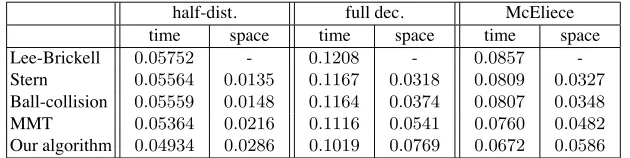
that this bound is tight foralmost alllinear codes, i.e.r =nH−1(1−R)+o(n). This justifies our choiceW =H−1(1−R)for the full decoding scenario. We conclude by taking a closer look at theworst-casecomplexities of decoding algorithms for random linear codes and a typical McEliece setting with relative distance D = 0.04 and rate R = 0.7577. Notice that three out of the four parameter sets for security levels between 80 and 256 bit from [3] closely match these code parameters.
half-dist. full dec. McEliece time space time space time space Lee-Brickell 0.05752 - 0.1208 - 0.0857 -Stern 0.05564 0.0135 0.1167 0.0318 0.0809 0.0327
Ball-collision 0.05559 0.0148 0.1164 0.0374 0.0807 0.0348
MMT 0.05364 0.0216 0.1116 0.0541 0.0760 0.0482
Our algorithm 0.04934 0.0286 0.1019 0.0769 0.0672 0.0586
Table 1: Comparison of worst-case complexity coefficients, e.g. the time columns represent the maximal complexity coefficientF(R)for0< R <1.
All algorithms were optimized for speed, not for memory. For a comparison of full decoding withfixed memory, we can easily restrict Ball-collision, MMT and our new algorithm to the space complexity coefficient 0.0317of Stern’s algo-rithm which holds fork≈0.446784. In this case, we obtain time complexities Fball(R) = 0.1163, FMMT(R) = 0.1129andFour(R) = 0.1110, which shows
that our improvement is not a pure time memory tradeoff.
http://cits.rub.de/personen/meurer.html. If needed, this code may also be used to compute optimal parameters for arbitrary code parameters.
Acknowledgment. We would like to thank Dan Bernstein for several excellent comments, in particular he proposed to use random partitions for generating the base lists in the COLUMNMATCH algorithm.
References
1. M. Alekhnovich. More on Average Case vs Approximation Complexity. In44th Symposium on Foundations of Computer Science (FOCS), pages 298–307, 2003
2. A. Becker, J.-S. Coron, and A. Joux. Improved generic algorithms for hard knapsacks. In EU-ROCRYPT, volume 6632 ofLecture Notes in Computer Science, pages 364–385. Springer, 2011.
3. D.J. Bernstein, T. Lange and C. Peters. Attacking and Defending the McEliece Cryp-tosystem. InPost-Quantum Cryptography, Second International Workshop, PQCrypto 2008, pages 31-46. Springer, 2008.
4. D. J. Bernstein, T. Lange, and C. Peters. Smaller decoding exponents: ball-collision de-coding. InCRYPTO, volume 6841 ofLecture Notes in Computer Science, pages 743–760. Springer, 2011.
5. R. J. M. Elwyn R. Berlekamp and H. C. van Tilborg. On the inherent intractability of certain coding problems. InIEEE Transactions on Information Theory, volume 24, pages 384–386, 1978.
6. V.M. Blinovskii. Lower asymptotic bound on the number of linear code words in a sphere of given radius inFn
q. InProbl. Peredach. Inform., vol 23, pages 50-53, 1987.
7. A. Canteaut and F. Chabaud. A new algorithm forfinding minimum-weight words in a linear code: Application to mceliece’s cryptosystem and to narrow-sense bch codes of length 511.
IEEE Transactions on Information Theory, 44(1):367–378, 1998.
8. J.T. Coffey and R.M. Goodman. The complexity of information set decoding. InIEEE Transactions on Information Theory, volume 36, pages 1031-1037, 1990.
9. J.T. Coffey and R.M. Goodman. Any code of which we cannot think is good. InIEEE Transactions on Information Theory, volume 36, 1990.
10. J.-C. Faug`ere, A. Otmani, L. Perret, and J.-P. Tillich. A Distinguisher for High Rate McEliece Cryptosystems. InYACC 2010, full version available as eprint Report 2010/331, 2010. 11. M. Finiasz and N. Sendrier. Security bounds for the design of code-based cryptosystems.
In M. Matsui, editor,Asiacrypt 2009, volume 5912 ofLecture Notes in Computer Science, pages 88–105. Springer, 2009.
12. T.J. Goblick, Jr. Coding for a discrete information source with a distortion measure. Ph.D. dissertation, Dept. of Elect. Eng., M.I.T., Cambridge, MA, 1962.
13. N.J. Hopper and M. Blum. Secure Human Identification Protocols. InLecture Notes in Com-puter Science, volume 2248, Proceedings ofAdvances in Cryptology - ASIACRYPT 2001, pages 52-66. Springer 2001.
14. N. Howgrave-Graham and A. Joux. New generic algorithms for hard knapsacks. In EU-ROCRYPT, volume 6110 ofLecture Notes in Computer Science, pages 235–256. Springer, 2010.
16. E. Kiltz, K. Pietrzak, D. Cash, A. Jain and D. Venturi. Efficient Authentication from Hard Learning Problems. InAdvances in Cryptology - EUROCRYPT 2011, pages 7-26. Springer, 2001.
17. D. Knuth. Art of Computer Programming, Volume 3: Sorting and Searching. Addison-Wesley Professional, 2 edition, 1998.
18. P. J. Lee and E. F. Brickell. An observation on the security of McEliece’s public-key cryp-tosystem. InAdvances in Cryptology - EUROCRYPT 1988, pages 275–280, 1988.
19. J. S. Leon. A probabilistic algorithm for computing minimum weights of large error-correcting codes.IEEE Transactions on Information Theory, 34(5):1354 – 1359, 1988. 20. L.B. Levitin. Covering radius of almost all linear codes satisfies the Goblick bound. InIEEE
Internat. Symp. on Information Theory, Kobe, Japan, 1988.
21. R. J. McEliece. A public-key cryptosystem based on algebraic coding theory. InJet Propul-sion Laboratory DSN Progress Report42–44, pages 114–116, 1978.
22. A. May, A. Meurer and E. Thomae. Decoding Random Linear Codes inO˜(20.054n) In
Asiacrypt 2011. Springer, 2011.To appear.
23. P. Q. Nguyen, I. E. Shparlinski, and J. Stern. Distribution of modular sums and the security of the server aided exponentiation. InProgress in Computer Science and Applied Logic, volume 20 ofFinal proceedings of Cryptography and Computational Number Theory work-shop, Singapore (1999), pages 331–224, 2001.
24. E. Prange. The Use of Information Sets in Decoding Cyclic Codes. IRE Transaction on Information Theory, volume 8, issue 5, pages 5-9, 1962.
25. C. Peters. Information-Set Decoding for Linear Codes overFq. InPost-Quantum
Cryptog-raphy, Third International Workshop, PQCrypto 2010, pages 81-94. Springer, 2010. 26. O. Regev. On lattices, learning with errors, random linear codes, and cryptography. In
Proceedings of the 37th Annual ACM Symposium on Theory of Computing (STOC), pages 84-93, 2005.
27. N. Sendrier. Finding the permutation between equivalent linear codes: The support splitting algorithm InIEEE Transactions on Information Theory, volume 46, pages 1193–1203, 2000. 28. N. Sendrier. On the security of the McEliece public-key cryptosystem. In M. Blaum, P. Far-rell, and H. van Tilborg, editors,Information, Coding and Mathematics, pages 141–163. Kluwer, 2002. Proceedings of Workshop honoring Prof. Bob McEliece on his 60th birthday. 29. J. Stern. A method forfinding codewords of small weight. InProceedings of the 3rd In-ternational Colloquium on Coding Theory and Applications, pages 106–113, London, UK, 1989. Springer-Verlag.
A A Provable Variant ofCOLUMNMATCH
In order to obtain a provable variant of the COLUMNMATCH algorithm, we consider the following variant PROVABLECM. Recover that one invocation of COLUMNMATCHrequires the random choice of three target vectorst(1)1 ∈Fr12 andt(2)1 ,t(2)3 ∈Fr2
2 .
Essentially, in PROVABLECM we repeatedly invoke COLUMNMATCHwith different independent target values t(ij) and add some artificial abort criteria that prevent the lists in the computation from growing unexpectedly strong. More detailed, for an integer parameter Λ ∈ N, we first choose random tar-get values t(1)1,i ∈ F(2r1) andt(2)1,j,t(2)3,k ∈ Fr22 for 1 ≤ i, j, k ≤ 8Λ and invoke
COLUMNMATCH(t(1)1,i,t(2)1,j,t(2)3,j) for all 1 ≤ i, j, k ≤ 8Λ until a solution is found. Furthermore, every single computation is aborted as soon as a list ex-ceeds its expected size by more than a factor of2γnfor afixed constantγ >0.
We now aim to prove the following
Theorem 1. For every γ >0, the modified algorithmPROVABLECM outputs a solution e ∈ Fk2+$, i.e.Qe = s and wt(e) = p, for a fraction of at least
1−60·2−γnrandomly chosenQ∈F$×(k+$)
2 with probability at least1−e32 > 12
in timeO˜!T(p, #;ε1, ε2)·23γn"whereT(p, #;ε1, ε2)is defined as in Eq.(4).
We make use of the following helpful theorem that can be obtained by a straightforward modification of the result in [23, Theorem 3.2].
Theorem 2. For a fixed matrix Q ∈ F2m×n, a target vector t ∈ Fm2 and an arbitrary setB ⊂Fn
2, we define
PQ(B,t) := 1
|B||{x∈ B : Qx=t}| .
Then for allB ⊂Fn
2 it holds that
1 2mn
#
Q∈Fm2×n
#
t∈Fm
2
(PQ(B,t)−21m)2 = 2
m−1
2m|B| .
The high-level idea for the proof of Theorem 1 is to consider the three dif-ferent nodes of decomposition as illustrated in Fig. 7. For every such node, we introduce a random variable Xi indicating whether the algorithm fails at this
point or not. The overall failure probability can then be upper bounded by using the union bound, i.e. Pr[PROVABLECM fails] ≤ &Pr[Xi = 0]. Hence, we
need to upper bound the failure probability of every single node. For this pur-pose, we divide everyXi into three eventsXij and setXi := -Xij. We now
– X11represents the event that for at least one choice of the{t(1)1,j}the solution
e ∈ Lhas at least one representation e = e1 +e2 with(Qe1)[r1] = t(1)1,j
and(Qe2)[r1]=s[r1]+t(1)1,j.
– X12 represents the event that for at least one choice of the{t(1)1,j}the size of listsL(1)1 andL(1)2 do not exceed the expected value by more than a factor of2γn.
– X3
1 represents the event that for at least one choice of the{t (1)
1,j}total number
of collisionsC1, see Sect.4, does not exceed it’s expected value by more than a factor of2γn.
. . .
L(1)1 L
(1) 2
L
X
2X
3X
1Fig. 7: Illustration of different decomposition nodes.
Basically, all these events depend on the structure of the matrixQand we need to exclude some pathological cases yielding clustered distributionsQe(for example the all-zero matrix). Hence, for all three events we define appropriate sets of “good” and “bad” matricesQwhich eventually allow to upper bound the failure probabilities of these events. Applying Theorem 2 allows to upper bound the fraction of bad matrices. The following three lemmas control the amount of bad matrices Qand target values t(i,jb)for every Xij. We omit the proofs which can be adopted from the proof of [2, Theorem 2] in a straightforward way.
Lemma 1. For all but a Λ1−1 fraction of theQ’s, the proportion of badt!sw.r.t. toX1
i is smaller thanΛΛ−1.
Lemma 2. For all but a (Λ2−Λ1)2 fraction of theQ’s, the proportion of bad t!s
w.r.t. toXi2is smaller than21Λ.
Using these lemmas, one can easily show that the total fraction of badQ’s for
oneof the three nodes can be bounded by
1
Λ−1 +
2Λ
(Λ−1)2 +
16
Λ ≤
20
Λ forΛ≥7
and hence the total fraction of badQ’s for all three nodes is upper bounded by 60
Λ. Furthermore, considering goodQ’s, the proportion of badt’s foronenode
is given by
Λ−1
Λ +
1 2Λ +
1
4Λ = 1−
1 4Λ and hence we have
Pr[Xi = 0] =Pr[all8Λmanyt’s bad]≤
'
1−41
Λ
(8Λ
≤e−2 .
Eventually this yields
Pr[PROVABLECM fails]≤ 3
e2
for every goodQas stated in the theorem. Notice, that the worst-case running time of PROVABLECMis given by a total number ofΛ3 = 23γninvocations of