A two-dimensional MHD model of the solar wind interaction with Mars
H. Shinagawa1and S. W. Bougher2
1Solar-Terrestrial Environment Laboratory, Nagoya University, Toyokawa 442-8507, Japan 2Lunar and Planetary Laboratory, University of Arizona, Tucson, Arizona 85721, U.S.A.
(Received August 7, 1997; Revised June 20, 1998; Accepted August 18, 1998)
The ionosphere of Mars is expected to be significantly affected by the solar wind because Mars does not possess a significant intrinsic magnetic field which deflects the solar wind. Despite a number of plasma measurements made near Mars, the nature of the solar wind-Mars interaction has not yet been fully understood. In order to self-consistently study the solar wind interaction with the ionosphere of Mars, a two-dimensional MHD model has been developed with an emphasis placed on the structure of the ionosphere of Mars. It is found that the modeled electron density profile in the upper ionosphere strongly depends on the solar wind dynamic pressure as well as the solar zenith angle. The ionosphere in the model tends to have an ionopause-like sharp drop of the electron density at some altitude for realistic solar wind dynamic pressures. Such behavior is not consistent with most of the observed electron density profiles, which exhibit relatively large and constant scale height in most of the dayside region. While the observed electron density profiles of the Venus ionosphere have been reproduced reasonably well by ionospheric models as well as recent three-dimensional MHD models, the electron density profiles of the Martian ionosphere have not been successfully reproduced by theoretical models including this study. This fact implies that processes not present in the Venus ionosphere, such as crustal magnetic fields and the rotation of the planet, may have significant effects on the structure and the dynamics of the ionosphere of Mars.
1.
Introduction
A number of electron density profiles of the Martian iono-sphere have been obtained by radio occultation measure-ments made by the Mariner and Viking orbiters (cf. Zhanget al., 1990; Kliore, 1992). Before the Mars Global Surveyor arrived at Mars, in situ measurements had been made only by the Viking landers, and the magnetic field had not been measured in the ionosphere. Recently the Mars Global Sur-veyor has detected a fairly strong (B ≤400 nT) but localized magnetic field which is thought to be of crustal origin (Acu˜na
et al., 1998). It has also been found that the surface magnetic field of core origin is likely to be smaller than about 5 nT, indicating that a global intrinsic magnetic field at Mars is un-likely to play an important role in the solar wind interaction with Mars.
A one-dimensional (1D) ionospheric model of Mars which includes the ionospheric magnetic field was developed by Shinagawa and Cravens (1989, 1992). In their model, the neutral density model based on the Viking 1 measurement was used. The observed ion density profiles were reproduced fairly well by the model, and the results suggested that an in-trinsic magnetic field at Mars is insignificant. However, the 1D ionospheric model is not capable of self-consistently in-cluding horizontal transport processes which are driven by the horizontal pressure gradient force as well as by the elec-tromagnetic force generated by the solar wind. The other problem is that the model has an upper boundary at a given altitude (480 km), and therefore the upper boundary
condi-Copy right cThe Society of Geomagnetism and Earth, Planetary and Space Sciences (SGEPSS); The Seismological Society of Japan; The Volcanological Society of Japan; The Geodetic Society of Japan; The Japanese Society for Planetary Sciences.
tions must have been given from the observations and theo-retical consideration. The upper boundary condition was also a problem with a two-dimensional (2D) ionospheric MHD model of Shinagawa (1996).
In order to model the structure of the Martian ionosphere including the solar wind interaction, we developed a 2D MHD model of the solar wind-Mars interaction. The model includes the ionosphere of Mars in more realistically than previous global models of solar wind-Mars interaction. The upper boundary has been extended to about seven radii from the center of Mars. There have been a number of studies of the solar wind-Venus interaction, suggesting that the iono-spheric structure of the non-magnetized planets is controlled mainly by the solar wind dynamic pressure (Psw). Thus, two
basic cases are examined in this paper: (1) highPsw, and (2)
lowPsw.
It must be noted that 2D modeling is not enough to accu-rately incorporate effects associated with three-dimensional (3D) configuration, such as tension of the magnetic field, horizontal transport of plasma along magnetic field lines. To study the interaction between the solar wind and the non-magnetized planets including such effects, 3D modeling is necessary. Recently, several groups developed 3D MHD models of the solar wind-Venus interaction (McGary and Pontius, 1994; Cable and Steinolfson, 1995; Murawski and Steinolfson, 1996a,b; Tanaka and Murawski, 1997). Among these studies, Tanaka and Murawski (1997) included the ionosphere of Venus and the solar wind simultaneously. The bow shock, the magnetic barrier, and the ionopause were re-produced realistically. The dynamics of the ionosphere of Venus was also reproduced reasonably well. Most recently, Tanaka (1998) has studied the solar wind interaction with
56 H. SHINAGAWA AND S. W. BOUGHER: A TWO-DIMENSIONAL MHD MODEL
the ionospheres of non-magnetized planets for two differ-ent solar wind conditions using a 3D MHD model with a two-component plasma. Tanaka and Murawski (1997) and Tanaka (1998) reported that the tension force becomes impor-tant near the terminator region. However, present 3D models treat the ionosphere in a very much simplified manner, and have not included the lower ionosphere, or O+2 ionosphere. We believe that 2D modeling still gives useful ideas in study-ing the ionosphere of Mars and its interaction with the solar wind.
2.
Model Description
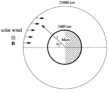
The 2D time-dependent single-fluid MHD equations, i.e., the continuity, momentum, energy, and magnetic induction equations are solved in a cylindrical coordinate system as shown in Fig. 1. The upper boundary is set at 25000 km from the center of Mars. The lower boundary is at 100 km above the surface, which is nearly the bottom of the ionosphere. Calculations are done for the upper half of the hemisphere, assuming axial symmetry with respect to the sun-Mars line. The left boundary is at the subsolar point, i.e., 0◦solar zenith angle (SZA), and the right boundary is at the antisolar point, i.e., SZA=180◦. The lower boundary conditions are given at 100 km, because at this altitude (i) photochemical equi-librium is a reasonable assumption for density, (ii) the ion velocity is considered to be the same as the neutral velocity which is assumed to be zero in this study, (iii) the plasma temperature is the same as the neutral temperature because of very large ion-neutral and electron-neutral collision fre-quencies, and (iv) the magneticfield at 100 km is zero. In the upper boundary condition, the density, velocity, mag-neticfield, and temperature of the solar wind are given in the upstream side, and gradients are taken to be zero for all variables in the downstream side.
The basic method of the modeling is the same as that of Shinagawa (1996). The solar wind magneticfield is assumed
Fig. 1. Coordinate system and region of the model. The cylindrical coor-dinate is used. The direction of the solar wind magneticfield is inzaxis and into the paper. The upper boundary is at 25000 km, and the lower boundary is at 3480 km which is 100 km above the surface of Mars.
to be perpendicular to the plane. In the continuity equation, the mass continuity equation is also included in addition to the number density equation. It is assumed that ions pro-duced in the ionosphere have 16 amu, i.e., mass of O+. The electron density is expressed as the sum of the O+density and the O+2 density. This procedure enables us to approxi-mately separate solar wind ions (H+) and ionospheric ions (O+). The ionosphere observed by the Viking landers indi-cated that the ions in the ionosphere consist of both O+2 and O+ (Hansonet al., 1977). If O+2 is included in the model, the scale height of the electron density would be slightly smaller. Artificial viscosity terms are added to all equations to maintain numerical stability.
Ionospheric parameters, such as ionization rates, chemi-cal reaction rates, are basichemi-cally the same as those used for 1D model (Shinagawa and Cravens, 1989, 1992), i.e., the parameters under the Viking conditions. A weak artificial ionization source (ionization rates are 10−4 of the dayside
values) is given on the nightside to prevent numerical insta-bility caused by extremely small densities. The radial grid size varies from 4 km near the lower boundary up to 500 km near the upper boundary. The angular grid size is 2.5◦for all SZAs. The grid size is 4 km at altitudes less than 480 km in vertical direction, which is enough to reproduce a fairly thin ionopause with a thickness of about 20 km. Effects of the rotation of Mars are not included in this study.
Two cases, Case 1 (high Psw) and Case 2 (low Psw), are
examined. For both Case 1 and Case 2, the solar wind plasma density, temperature, and magnetic field are taken to be 5 cm−3, 2×10⁵K, and 3 nT, respectively. The solar
wind velocity Vswis taken to be 450 km/s for Case 1 and
300 km/s for Case 2. Starting from practically zero densities in the modeling region, the system approximately reached a steady state in about three hours.
3.
Results
3.1 Case 1 (HighPsw)
The solar wind velocity (Vsw) is 450 km/s, and the solar
wind density is 5 cm−3, giving a solar wind dynamic pressure (Psw) of about 1.7×10⁻⁸dyne/cm2. Under this condition,
Pswconsiderably exceeds the maximum ionospheric thermal
pressure (Pi) of Mars which is about 5×10⁻⁹dyne/cm2in
this model. The Pioneer Venus observations confirmed that in the solar wind-Venus interaction for the case ofPsw>Pi,
most of the dayside ionosphere becomes strongly magne-tized and compressed, and the ionopause height becomes low (cf. Elphicet al., 1981). This type of the ionosphere has been reproduced by both 2D and 3D models reasonably well (Shinagawa, 1996; Tanaka and Murawski, 1997; Tanaka, 1998).
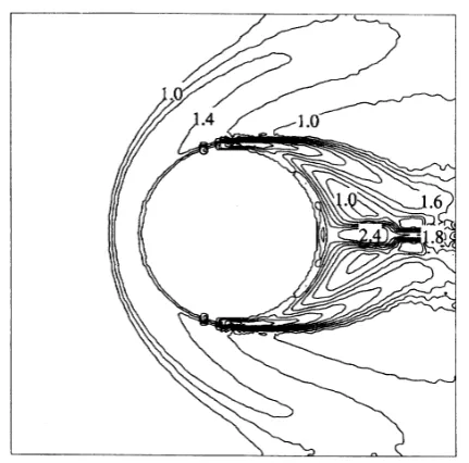
The modeled ionosphere of Mars appears to be analogous to the Venus ionosphere for Psw > Pi. Figure 2 shows the
contour plot of the calculated electron densities around Mars in logarithm of particle number in cubic centimeters. The solar wind is flowing from the left-hand side to the right-hand side. A bow shock is formed at about 1.4RM, which is
Fig. 2. Contour plot of the calculated electron densities in cubic centimeters in logarithmic scale for Case 1. Contour lines are not plotted near the surface of Mars (z<500 km).
Fig. 3. Contour plot of the calculated electron densities below 500 km in cubic centimeters in logarithmic scale for Case 1.
cannot be seen in Fig. 2. On the nightside, a weak ionosphere with the electron density of 101–102 cm−3 extends up to
the wake region, forming an“ionotail”. The overall plasma structure in this model is similar to that of the 3D study by Tanaka (1998).
The calculated electron density in the ionosphere is shown in the contour in Fig. 3. Ions in the topside ionosphere are removed by strong downward and day-to-night convec-tion driven by the solar wind dynamic pressure. It is found that an ionopause is formed at an altitude of about 170 km from SZA =0◦ to SZA= 60◦. The ionopause height in-creases rapidly with SZA for SZA>60◦. The“low-altitude ionopause”is commonly observed in the Venus ionosphere when the solar wind dynamic pressure exceeds the iono-spheric thermal pressure (Elphicet al., 1981). In the ter-minator region, there is a small day-to-night ion transport,
Fig. 4. Contour plot of the calculated magneticfield strength in nanotesla for Case 1.
Fig. 5. Contour plot of the magneticfield strength in nanotesla at altitudes below 500 km for Case 1.
but it is not enough to maintain the significant nightside ionosphere. A weak nightside ionosphere of 103 cm−3 is
maintained primarily by artificially ionization source in this model. This is not necessarily unrealistic because in the case of the nightside ionosphere of Venus the electron density of 103–104cm−3is thought to be maintained by ionization due
to particle precipitation.
bot-58 H. SHINAGAWA AND S. W. BOUGHER: A TWO-DIMENSIONAL MHD MODEL
Fig. 6. Altitude profile of the plasma thermal pressure, the magnetic pres-sure, and the total pressure in the ionosphere for Case 1 in the unit of 10−10dyne/cm2.
tom of the ionosphere, the magneticflux is removed by the magnetic diffusion because of large resistivity. The mag-neticfield strength decreases rapidly with SZA, and becomes nearly zero in the nightside ionosphere. A weak magnetic field in the region beyond the terminator is the result of a numerical diffusion effect on the magneticfield.
The altitude profiles of the plasma thermal pressure, the magnetic pressure, and the total pressure at the subsolar point are shown in Fig. 6. The pressure is in the form of plasma thermal pressure above 200 km. In this region, the plasma density is low, but the temperature is high. Below 200 km temperature becomes low because of thermal energy is lost by the ion-neutral collisions. The magnetic pressure becomes high at about 170 km. The magneticfield is removed through magnetic diffusion at low altitudes. The total pressure gra-dient force is balanced with the ion-neutral drag force at the bottom of the ionosphere. The solar wind dynamic pressure is converted to the plasma thermal pressure and the magnetic pressure at the bow shock. Then, the magnetic pressure be-comes dominant in the lower magnetosheath region which is sometime called the magnetic barrier region. In the lower ionosphere, the magnetic pressure is balanced with the iono-spheric thermal pressure plus the ion-neutral drag force.
3.2 Case 2 (LowPsw)
A case for the solar wind velocity of 300 km and the density of 5 cm−3, is also investigated. The dynamic pressure is now about 7.5×10⁻⁹ dyne/cm2, which is lower and more common than Case 1. The electron density in this ionosphere for this case is shown in the contour plot of Fig. 7. The height of ionopause is about 180 km in the subsolar region, and increases rapidly with SZA because of rapid decrease of ramPswexerting on the ionosphere. The ionopause appears
at higher altitudes at all SZAs than that of Case 1, but the thickness is still relatively small. The ionospheric thermal
Fig. 7. Contour plot of the calculated electron densities below 500 km in cubic centimeters in logarithmic scale for Case 2.
Fig. 8. Contour plot of the magneticfield strength in nanoteslas at altitudes below 500 km for Case 2.
pressure is now sufficient to hold the solar wind dynamic pressure except in the subsolar region.
There is a day-to-night ion transport, but unlike the Venus ionosphere, the ion flux is smaller mainly because of the lower density in the dayside ionosphere. The ion density in the nightside ionosphere is of the order of 103 cm−3. The
calculated magneticfield in the ionosphere is shown in the contour plot (Fig. 8). The maximum of the magneticfield strength is now 30 nT at about 270 km. The overall behavior of the magneticfield for Case 2 is similar to that for Case 1.
Fig. 9. Altitude profile of the plasma thermal pressure, the magnetic pres-sure, and the total pressure in the ionosphere for Case 2 in the unit of 10−10dyne/cm2.
4.
Discussion
The Viking observations confirmed that the ionospheric peak plasma pressure observed by the Viking landers is sig-nificantly smaller than the average solar wind dynamic pres-sure, indicating that the ionospheric magneticfield compen-sates for the missing pressure at least under the Viking con-ditions (Hanson and Mantas, 1988). The question then was whether this ionospheric magneticfield is an intrinsic mag-neticfield or an induced magnetic field by the solar wind. The answer has recently been given by the Mars Global Sur-veyor which found that the surface magneticfield of a global intrinsic magneticfield is likely to be smaller than about 5 nT (Acuna˜ et al., 1998). Thus, the magneticfield of core origin is unlikely to be a dominant magneticfield in the ionosphere, and the ionosphere of Mars can be considered to befilled with the magneticfield induced by the solar wind. Since the magnitude of the intrinsic magneticfield at Mars is found to be small, the nature of the solar wind-Mars interaction should be analogous to that of the solar wind-Venus interac-tion. The question now is whether or not theoretical models based on the idea of the solar wind-Venus interaction are able to reproduce the plasma environment of Mars.
Vertical profiles of the calculated electron density are shown in Fig. 10 along with the electron densities obtained by the Viking 1 and 2 landers. Case 1 and Case 2 are the cases forVsw=450 km/s and 300 km/s, respectively. V1 and V2
denote the electron density profiles of the Viking 1 and 2 lan-ders, respectively. As is shown in Figs. 3, 5, and 8, both for Case 1 and Case 2 an ionopause is seen. The ionopause is cre-ated by the combination of downward motion and horizontal transport process, as was discussed for the Venus ionosphere (Cravens and Shinagawa, 1991; Shinagawa, 1996; Tanaka and Murawski, 1997; Tanaka, 1998). However, the radio occultation measurements made by the Mariner and Viking
Fig. 10. Altitude profiles of the calculated electron densities at solar zenith angle (SZA) = 45◦ for Case 1 and Case 2. V1 and V2 denote the observed electron density profiles obtained by the Viking 1 and 2 landers, respectively.
orbiters indicate that most of the observed electron density profiles have fairly constant and relatively large plasma scale height at all altitudes, exhibiting no clear ionopause structure (Zhanget al., 1990; Kliore, 1992).
In the Venus ionosphere forPsw>Pi, a strong convection
is believed to be driven in the ionosphere, giving a very small plasma scale height above the photochemical region. On the other hand, most of the electron density profiles observed obtained by previous measurements appear to be fairly stable and have fairly large and constant scale height on the dayside (Kliore, 1992). Krymskiiet al.(1995) pointed out that the scale height of the Martian ionosphere should be significantly smaller than the observed one, if the magnitude of plasma convection in the Martian ionosphere is as large as that in the Venus ionosphere. A recent 3D study of Tanaka (1998) also tends to produce a smaller scale height than the observed one under the condition ofPsw>Pi, although the 3D model
treats the lower part of the ionosphere rather crudely. The result in our study is consistent with the 3D study.
Recently the Mars Global Surveyor has discovered fairly strong (B ≤ 400 nT) but highly localized magneticfields which are probably of crustal origin at various places (Acuna˜
60 H. SHINAGAWA AND S. W. BOUGHER: A TWO-DIMENSIONAL MHD MODEL
5.
Summary
Structure of the ionosphere associated with the solar wind interaction with Mars was investigated using the 2D MHD model which includes the solar wind. Although the 2D model has various limitations in quantitatively reproducing physical processes around Mars, the modeled profiles of the electron density and the magneticfield give some idea of the iono-spheric processes.
In the 2D model, a clear and relatively sharp ionopause is always formed in the dayside ionosphere for realistic solar wind parameters. This result is consistent with recent 3D study (Tanaka, 1998). Like the ionosphere of Venus, the ionopause altitude changes with SZA as well as the solar wind dynamic pressure. This behavior, however, is not con-sistent with most of the observations made by the Mariner and Viking spacecraft, which rarely observed clear ionopause-like structure. This fact suggests that processes not present in the Venus ionosphere, such as crustal magneticfields and the rotation of the planet, may have significant effects on the structure and the dynamics of the ionosphere of Mars.
In spite of very small intrinsic magneticfield, the Martian plasma environment appears to be somewhat different from Venus. In addition to the solar wind-induced magneticfield and magneticfields of crustal origin and/or effects of the ro-tation of Mars might play a significant role in determining the structure and dynamics of the ionosphere of Mars. Ob-servations of the upper atmosphere by NOZOMI, which was launched in the summer of 1998, along with further model-ing studies will give a clue to understand the nature of the solar wind interaction with Mars.
Acknowledgments. This work was done using computers of the Nagoya University Computing Center.
References
Acuna, M. H., J. E. P. Connerney, P. Wasilewski, R. P. Lin, K. A. Anderson,˜
C. W. Carlson, J. McFadden, D. W. Curtis, D. Mitchell, H. Reme, C. Mazelle, J. A. Sauvaud, C. d’Uston, A. Cros, J. L. Medale, S. J. Bauer, P. Cloutier, M. Mayhew, D. Winterhalter, and N. F. Ness, Magneticfield and plasma observations at Mars: Initial results of the Mars Global Surveyor mission,Science,279, 1676–1680, 1998.
Bougher, S. W. and H. Shinagawa, The Mars thermosphere-ionosphere: Predictions for the arrival of Planet-B,Earth Planets Space,50, 247–
257, 1998.
Cable, S. and R. S. Steinolfson, Three dimensional MHD simulations of the interaction between Venus and the solar wind,J. Geophys. Res.,100, 21645–21658, 1995.
Cravens, T. E. and H. Shinagawa, The ionopause current layer at Venus,J.
Geophys. Res.,96, 11119–11131, 1991.
Dolginov, Sh. and L. N. Zhuzgov, The magneticfield and the magnetosphere of the planet Mars,Planet. Space Sci.,39, 1493–1510, 1991.
Elphic, R. C., C. T. Russell, J. G. Luhmann, F. L. Scarf, and L. H. Brace, The Venus ionopause current sheet: Thickness length scale and controlling factors,J. Geophys. Res.,86, 11430–11438, 1981.
Hanson, W. B. and G. P. Mantas, Viking electron temperature measurements: Evidence for a magneticfield in the Martian ionosphere,J. Geophys. Res., 93, 7538–7544, 1988.
Hanson, W. B., S. Sanatani, and D. R. Zuccaro, The Martian ionosphere as observed by the Viking retarding potential analyzers,J. Geophys. Res., 82, 4351–4363, 1977.
Kliore, A. J., Radio occultation observations of the ionospheres of Mars and Venus, inVenus and Mars: Atmospheres, Ionospheres, and Solar Wind Interactions, edited by J. G. Luhmann, M. Tatrallyay, and R. O. Pepin, Geophysical Monograph Series, 66, pp. 265–276, American Geophysical Union, Washington, D.C., 1992.
Krymskii, A. M., T. Breus, and E. Nielsen, On possible observational ev-idence in electron density profiles of a magneticfield in the Martian ionosphere,J. Geophys. Res.,100, 3721–3730, 1995.
McGary, J. E. and D. H. Pontius, Jr., MHD simulations of boundary layer formation along the dayside Venus ionopause due to mass loading,J. Geophys. Res.,99, 2289–2300, 1994.
Murawski, K. and R. S. Steinolfson, Numerical simulations of mass loading in the solar wind interaction with Venus,J. Geophys. Res.,101, 2547–
2560, 1996a.
Murawski, K. and R. S. Steinolfson, Numerical modeling of the solar wind interaction with Venus,Planet. Space Sci.,44, 243–252, 1996b. Schwingenschuh, K., W. Riedler, H. Lichtennegger, Ye. Yeroshenko, K.
Sauer, J. G. Luhmann, M. Ong, and C. T. Russell, Martian bow shock: Phobos observations,Geophys. Res. Lett.,17, 889–892, 1990. Shinagawa, H., A two-dimensional MHD model of the solar wind interaction
with the Venus ionosphere,COSPAR Colloq. Ser.,4, 199–202, 1993. Shinagawa, H., A two-dimensional model of the Venus ionosphere: 2.
Mag-netized ionosphere,J. Geophys. Res.,101, 26921–26930, 1996. Shinagawa, H. and T. E. Cravens, A one-dimensional multi-species
magne-tohydrodynamic model of the dayside ionosphere of Mars,J. Geophys. Res.,94, 6506–6516, 1989.
Shinagawa, H. and T. E. Cravens, The ionospheric effects of a weak intrinsic magneticfield at Mars,J. Geophys. Res.,97, 1027–1035, 1992. Slavin, J. A. and R. E. Holzer, The solar wind interaction with Mars revisited,
J. Geophys. Res.,87, 10285–10296, 1982.
Tanaka, T., Effects of decreasing ionospheric pressure on the solar wind interaction with non-magnetized planets,Earth Planets Space,50, 259–
268, 1998.
Tanaka, T. and K. Murawski, Three-dimensional MHD simulations of the solar wind interaction with the ionosphere of Venus: Results of two-component reacting plasma simulation,J. Geophys. Res.,102, 19805–
19821, 1997.
Zhang, M. H. G., J. G. Luhmann, A. J. Kliore, and J. Kim, A post-Pioneer Venus reassessment of the Martian dayside ionosphere as observed by radio occultation methods,J. Geophys. Res.,95, 14829–14839, 1990.