Sequential estimation of intrinsic activity and synaptic input in single neurons by particle filtering with optimal importance density

R E S E A R C H

Open Access

Sequential estimation of intrinsic activity

and synaptic input in single neurons by particle

filtering with optimal importance density

Pau Closas

and Antoni Guillamon

Abstract

This paper deals with the problem of inferring the signals and parameters that cause neural activity to occur. The ultimate challenge being to unveil brain’s connectivity, here we focus on a microscopic vision of the problem, where single neurons (potentially connected to a network of peers) are at the core of our study. The sole observation available are noisy, sampled voltage traces obtained from intracellular recordings. We design algorithms and inference methods using the tools provided by stochastic filtering that allow a probabilistic interpretation and treatment of the problem. Using particle filtering, we are able to reconstruct traces of voltages and estimate the time course of auxiliary variables. By extending the algorithm, through PMCMC methodology, we are able to estimate hidden physiological parameters as well, like intrinsic conductances or reversal potentials. Last, but not least, the method is applied to estimate synaptic conductances arriving at a target cell, thus reconstructing the synaptic excitatory/inhibitory input traces. Notably, the performance of these estimations achieve the theoretical lower bounds even in spiking regimes.

Keywords: State-space models, Inference and learning, Particle filtering, Synaptic conductance estimation, Spiking neuron, Conductance-based model, Intracellular recording

1 Introduction

Measurements of membrane potential traces constitute the main observable quantities to derive a biophysical neuron model. In particular, the dynamics of auxiliary variables and the model parameters are inferred from volt-age traces, in a costly process that typically entails a vari-ety of channel blocks and clamping techniques (see, for instance, [1]), as well as some uncertainty in the param-eter values due to noise in the signal. Recent works in the literature deal with the problem of inferring hidden parameters of the model; see, for instance, [2–4] and, for an exhaustive review, [5]. In the same line, attempts to extract connectivity in networks of neurons from calcium imaging, see [6], are worth mentioning.

Apart from inferring intrinsic parameters of the model, voltage traces are also useful to obtain valuable informa-tion about synaptic input, an inverse problem with some satisfactory (see, for instance, [7–13]) but no complete

*Correspondence: [email protected]

1_{Northeastern University, Boston, MA 02115, USA}

Full list of author information is available at the end of the article

solutions yet. The main shortcomings are the requirement of multiple (supposedly identical) trials for some methods to be applied and the need of avoiding signals obtained when ionic currents are active. The latter constraint arises from the fact that many methods rely on the linearity of the signal and this is not possible to achieve under quite general situations, like spiking regimes (see [14]) or sub-threshold regimes when specific currents (e.g., AHP, LTS) are active (see [15]).

The problem investigated in this paper considers recordings of noisy voltage traces to infer the hidden gating variables of the neuron model, as well as filtered voltage estimates, model parameters, and input synaptic conductances.

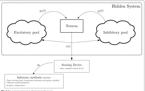
Figure 1 shows the basic setup we are dealing with in this article. The neuron under observation has its own dynamics, producing electrical voltage patterns. The gen-eration of action potentials is regulated by internal drivers (e.g., the active gating variables of the neuron) as well as exogenous factors like excitatory and inhibitory synaptic conductances produced by pools of connected neurons. This system is unobservable, in the sense that we cannot

Fig. 1The experimental setup of interest in this paper

measure it directly. The sole observation from this system are the noisy membrane potentialsyk. In this experimen-tal scenario, the ultimate goal is to extract the following quantities:

1. The time-evolving states characterizing the neuron dynamics, including a filtered membrane potential and the dynamics of the gating variables

2. The parameters defining the neuron model 3. The dynamics of synaptic conductances and its

parameters, the final goal being to discern the temporal contributions of global excitation from those of global inhibition,gE(t)andgI(t), respectively.

An ideal method should be able to sequentially infer the time course of the membrane potential and its intrin-sic/extrinsic activity from noisy observations of a voltage trace. The main features of the envisaged algorithm are fivefold: (i)Single-trial: the method should be able to esti-mate the desired signals and parameters from a single voltage trace, thus avoiding the experimental variability among trials; (ii)Sequential: the algorithm should provide estimates each time a new observation is recorded, thus avoiding re-processing of all data streams each time; (iii) Spike regime: contrary to most solutions operating only under the subthreshold assumption, the method should

be able to operate in the presence of spikes as well; (iv) Robust: if the method is model-dependent, thus implying knowledge of the model parameters, then the algorithm should be provided with enhancements to adaptively learn these parameters; and (v)Statistically efficient: the perfor-mance of the method should be close to the theoretical lower bounds, meaning that the estimation error cannot be substantially reduced. Notice that the focus here is not on reducing the computational cost of the inference method, and thus, we allow ourselves to use resource-consuming algorithms. Indeed, the target application does not demand (at least as a main requirement) real-time operation, and thus, we prioritized performance (i.e., esti-mation accuracy and the rest of features described earlier) in our developments.

therein includes a discussion of the discrete state-space representation of the problem and the model inaccuracies due to mismodeling effects. We present two sequential inference algorithms: (i) a method based on particle filter-ing (PF) to estimate the time-evolvfilter-ing states of a neuron under the assumption of perfect model knowledge and (ii) an enhanced version where model parameters are jointly estimated, and thus, the rather strong assumption of per-fect model knowledge is relaxed. We provide exhaustive computer simulation results to validate the algorithms and observe that they are attaining the theoretical lower bounds of accuracy, which are derived in the paper as well. In this paper, we use the powerful tools of PF to make inferences in general state-space models. PF are a set of methods able to sample from the marginal filtering dis-tribution in situations where analytical solutions are hard to work out or simply impossible. In the recent years, PFs played an important role in many research areas such as signal detection and demodulation, target tracking, posi-tioning, Bayesian inference, audio processing, financial modeling, computer vision, robotics, control, or biology [18–24]. At a glance, PF approximates the filtering distri-bution of states given measurements by a set of random points, properly weighted according to Bayes’ rule. The generation of the random particles can be done through a variety of distributions, known as importance den-sity. Particularly, we formulate the problem at hand and observe that it is possible to use the optimal importance density [25]. This distribution generates particles close to the target distribution, and thus, it can be shown to reduce the variance of the particles. As a consequence, for a fix number of particles, usage of this approach (not always possible) leads to better accuracy results than other choices. To the authors’ knowledge, the utilization of such sampling distribution is novel in the context of neural model filtering. Similar works have used PF to track neu-ral dynamics, but with no optimal importance density (see [2, 3, 26]), or to estimate synaptic input from sub-threshold recordings [11], as opposite to our proposed approach where we aim at providing estimates during the, highly nonlinear, spike regime. These references use the expectation-maximization algorithm to estimate the model parameters. In this paper, we use the Particle Marginal Markov-Chain Monte-Carlo (PMCMC) method to estimate the parameters. Lighter filtering methods based on the Gaussian assumption were considered in the literature (see [12, 13, 27] for instance), but the assump-tion might not hold in general, for instance, due to outliers in the membrane measurements or if more sophisticated models for the synaptic conductances are considered. In these situations, a PF approach seems more appropri-ate. As mentioned earlier, the focus here is on highly efficient and reliable filtering methods, rather than on computationally light inference methods. Summing up,

our method jointly treats the features of handling single-voltage traces governed by nonlinear models, estimating both neuron parameters and synaptic conductances, even in the spiking regimes, and using optimal importance den-sity for the PF together with a MCMC algorithm. The above references cope with some of these features, but to our knowledge, none of the recent methods in the lit-erature accounts for all of them. It is worth noting that other simulation-based solutions can be adopted besides the PMCMC. For instance, the works [28–32] tackle state estimation and model fitting problems jointly.

The remainder of the article is organized as follows. In Section 2, we expose the problem and present the statistical model, essentially a discretization of the well-known Morris-Lecar model, and we analyze the model inaccuracies as well. Next, in Section 3, we present the different inference algorithms we apply depending on the knowledge of the system. Results are given in Section 4, where we tackle three inference problems: (i) when the parameters defining the model are known; (ii) when the parameters of the model are unknown, and thus, they need to be estimated; and (iii) estimation of synaptic con-ductances from voltage traces assuming unknown model parameters. Finally, Section 5 concludes the paper with final remarks.

2 Problem statement and model

2.1 Measurement modeling

The recording of the membrane potential is a physi-cal process, including some approximations/inaccuracies involving:

1. Voltage observations are noisy. This is due, in part, to the thermal noise at the sensing device, non-ideal conditions in experimental setups, etc.

2. Recorded observations are discrete. All sensing devices record data by sampling at discrete time-instantsk, at a sampling frequencyfs=1/Ts,

the continuous-time natural phenomena. This is the task of an Analog-to-Digital Converter (ADC). Moreover, these samples are typically digitized, i.e., expressed by a finite number of bits. This latter issue is not tackled in the work as we assume that modern computer capabilities allow us to sample with relatively large number of bits per sample.

The problem can thus be posed in the form of a discrete-time, state-space model, where the observations are

yk∼N

vk,σy2,k

, (1)

signal-to-noise ratio (SNR) as SNR=Ps/Pn, withPsbeing the average signal power andPn=σ_y2_,kthe noise power.

2.2 Neural dynamical system

The methods presented in this paper rely on continuous models for the evolution of the voltage-traces and the hidden variables of a neuron. Our reference framework are conductance-based models endowed with a synaptic input termIsynand an (steady) applied currentIapp, that is, equations of type

Cmv˙= −¯gL(v−EL)−

is the time-varying ionic current for the jth ionic species, J = {Na, K, Cl, Ca,. . .}, where g¯j is the maximal conductance,pj involves the so-called gat-ing variables, and Ej is the reversal potential of the ionic channel. The synaptic input is expressed asIsyn = gE(t)(v(t)−EE)+gI(t)(v(t)−EI). We use the so-called effective point-conductancemodel, see [7, 33], where the excitatory/inhibitory global conductances are treated as Ornstein-Uhlenbeck (OU) processes Gaussian process with unit variance. Then, the OU pro-cess has meangu,0, standard deviationσu, and time con-stantτu. This simple model was shown in [33] to yield a valid description of the synaptic noise, capturing the prop-erties of more complex models. Other dynamics could be considered instead.

Concerning the neuron model, that is, the equation Cmv˙= −¯gL(v−EL)−j∈J Ij, in this work, we focus on the Morris-Lecar model [34] for the sake of clarity, which is able to model a wide variety of neural dynamics; see [35]. Details of the Morris-Lecar model can be found in Appendix 1. The unknown state vector in this case is com-posed of the membrane potential,v, and a unique ionic (K+-)current involving the gating variablen. We write

xk = _nvk k

. (4)

Notice that the Morris-Lecar neuron model is defined by a system of continuous-time, ordinary differential equations (ODEs) of the formx˙ =f(x). In general, mathe-matical models for neurons are of this type. However, due to the sampled recording of measurements, we are inter-ested in expressing the model in the form of a discrete state-space,

xk =fk(xk−1)+νk (5)

whereνk ∼N(0,x,k)is the process noise which includes the model inaccuracies. The covariance matrix x,k is used to quantify our confidence in the model that maps fk :{vk−1,nk−1} → {vk,nk}. In general, obtaining a closed-form analytical expression forfkwithout approximations is not possible. In such a case, we could use the Euler method:

which is of the Markovian type.

If we focus on the Morris-Lecar model, the resulting discrete version of the ODE system in (40)–(41) is:

vk = vk−1−

The goal is to express the inference problem in state-space formulation and apply stochastic filtering tools learned from signal processing. The final ingredient to do so is to introduce the so-called process noise in the state equation. Leveraging on the observation equation in (1), the state-space can be formulated as

xk = fk Gaussian with covariance matrixx,k. Further details of this matrix are discussed in Section 2.4. The measure-ment noiseνy,kis assumed zero-mean, Gaussian, and with variance σ_y2_,k. Notice that the system is characterized by Gaussian distributions and is linear in the observations; this allows for an optimal design of the proposal density in the PF as exploited in Section 3.1.

the OU stochastic process in (3) describing Isyn. There-fore, the continuous-time state isx = (v,n,gE,gI). The discrete version of the state-space is used again.

2.4 Model inaccuracies

The proposed estimation method relies on the fact that the neuron model is known. This is true to some extent, but most of the parameters in the Morris-Lecar model discussed are to be estimated. Typically, this model cal-ibration is done beforehand, but as we will see later in Section 3.2, this could be done in parallel to the filtering process. Therefore, the robustness of the method to pos-sible inaccuracies should be assessed. In this section, we point out possible causes of mismodeling. Computer sim-ulations are later used to characterize the performance of the proposed methods under these impairments.

In the single-neuron model considered, three major sources of inaccuracies can be identified. First, the applied current Iapp can be itself noisy, with a variance depend-ing on the quality of the instrumentation used and the experiment itself. We model the actual applied current as a random variable

Iapp=Io+νI,k, νI,k ∼N

0,σ_I2 , (12)

whereIois the nominal current applied andσI2the vari-ance around this value. Plugging (12) into (8), we obtain that the contribution ofIappto the noise term is_CT_msνI,k ∼ N0,(Ts/Cm)2σI2

.

Secondly, when the conductance of the leakage term is estimated beforehand, some inaccuracies might be taken into account. In general, this term is considered con-stant in the models although it gathers relatively distinct phenomena that can potentially be time-varying. The maximal conductance of the leakage term is therefore inaccurate and modeled as

¯

gL= ¯gLo+νg,k, νg,k∼N

0,σ_g2, (13)

whereg¯_Lo is the nominal, estimated conductance and σ_g2 the variance of this estimate. Similarly, inserting (13) into (8), we see that the contribution ofg¯Lto the noise term is

Ts are to be estimated. In general, these parameters can be properly obtained off-line by standard methods; see [36]. However, as they are estimates, a residual error typically remains. To account for these inaccuracies, we consider that the equation governing the evolution of gating vari-ables is corrupted by a zero-mean additive white Gaussian process with varianceσ_n2.

This analysis allows us to construct a realistic_x,k, as the contribution of the aforementioned inaccuracies. In a practical setup, in order to compute the noise variance due to leakage, we need to use the approximationvˆk−1≈

vk−1, wherevˆk−1is estimated by the filtering method. We construct the covariance matrix of the model as

x,k= σ

where we used that the overall noise in the voltage model is Ts

as an estimate ofσ_v2, provided accurate knowledge ofσ_I2 andσ_g2. Otherwise, the covariance matrix of the process could be estimated by other means, as the ones presented in Section 3.2 for mixed state-parameter estimation in nonlinear filtering problems.

Notice that we are implicitly assuming white processes due to the diagonal structure of x,k. It is worth men-tioning that, should correlated noise be a more realistic model, the method proposed in this article would be still valid. The proposed method can cope with colored noise statistics since x,k can be used seamlessly if it is not diagonal.

3 Methods

Two filtering methods are proposed here, depending on the knowledge regarding the underlying dynamical model. Section 3.1 presents an algorithm able to estimate the states inxk by a PF methodology, the particularity being that an optimal distribution is used to draw the random samples characterizing the joint filtering distribution of interest. This method assumes knowledge of the param-eter values of the system model, although we account for some inaccuracies as detailed in Section 2.4. An enhanced version of this method is presented in Section 3.2, where we relax the assumption of knowing the parameter val-ues. Leveraging on a PMCMC algorithm and the use of the optimal importance density as in the first method, we present a method that is able to filterxk while estimating the values describing the neuron model.

3.1 Sequential estimation of voltage traces and gating variables

The type of problems we are interested in involve the estimation of time-evolving signals that can be expressed through a state-space formulation. Particularly, estima-tion of the states in a single-neuron model from noisy voltage traces can be readily seen as a filtering problem. Bayesian theory provides the mathematical tools to deal with such problems in a systematic manner. The focus is on sequential methods that can incorporate new available measurements as they are recorded without the need for reprocessing all past data.

based on all available measurements,y1:k =

y1,. . .,yk

. To that aim, we are interested in the filtering distribution p(xk|y1:k). Assuming the Markovian property in (10) and (11), the distribution can be recursively expressed as

p(xk|y1:k)= and the prior distributions, respectively. Unfortunately, (16) can only be obtained in closed-form in some spe-cial cases, and in more general setups, we should resort to more sophisticated methods. In this paper, we consider PF to cope with the nonlinearity of the model. Although other lighter approaches might be possible as well [22], we seek the maximum accuracy regardless the involved computa-tional cost. Theoretically, for sufficiently large number of particles, particle filters offer such performances.

Particle filters, see [18, 20, 21, 23], approximate the filtering distribution by a set ofNweighted random

sam-ples, forming the random measure

x(_ki),w(_ki) N

i=1. These random samples are drawn from the importance density distribution,π(·),

and weighted according to the general formulation

w(_ki)∝w(_ki₋)₁

py_k|x(_0:i)_k,y_1:k−1px(_ki)|x(_ki₋)₁

πx(_ki)|x_0:(i)_k−1,y1:k

. (18)

The importance density from which particles are drawn is a key issue in designing efficient PFs. It is well known that the optimal importance density is

πxk|x_0:(i)_k−1,y1:k

=pxk|x(_ki₋)₁,yk

,

in the sense that it minimizes the variance of importance weights. Weights are then computed using (18) asw(_ki) ∝

w(_ki₋)₁pyk|x(_ki₋)₁

. This choice requires the ability to draw

fromp(xk|x(_ki₋)₁,yk)and to evaluatep

yk|x(_ki₋)₁

. In gen-eral, the two requirements cannot be met, and one needs to resort to suboptimal choices. However, given the partic-ular structure of the state-space model, we are able to use the optimal importance density. The fact that the model is Gaussian and the observations are related linearly to states allow to solve for the conditional distribution of states from the joint Gaussian distribution of states and observations. The equations are:

pxk|x(_ki₋)₁,yk

and the importance weights can be updated using

p tion of the filtering distribution of the form

p(xk|y1:k)≈

which gathers all information fromxk that the measure-ments up to timekprovide. The minimum mean square error estimator can be obtained as

ˆ in this section could be easily adapted to other neuron models by simply substituting the corresponding tran-sition function fk and constructing the state vector xk accordingly.

As a final step, PFs incorporate a resampling strat-egy to avoid the collapse of particles into a single state point. Resampling consists in eliminating particles with low importance weights and replicating those in high-probability regions [37]. The overall algorithm can be looked up in Algorithm 1 at instancek. Notice that this version of the algorithm requires knowledge of noise statistics and all the model parameters, which for the Morris-Lecar model are

=g¯L,EL,g¯Ca,ECa,g¯K,EK,φ,V1,V2,V3,V4

. (24)

When we add the dynamics of the synaptic conduc-tances, the vectorof model parameters also includesτE,

τI,gE,0,gI,0,σE, andσI.

3.2 Joint estimation of states and model parameters

In practice, the parameters in (24) might not be known. It is reasonable to assume that , or a subset of these parametersθ ⊆, are unknown and need to be estimated at the same time the filtering method in Algorithm 1 is executed. Therefore, the ultimate goal in this case is to estimate jointly the time evolving states and the unknown parameters of the model,x1:kandθ, respectively.

Algorithm 1 Particle filtering with optimal importance

handle in the context of PFs. Refer to [38–40] and their references for a complete survey. Here, we follow the approach in [41] and make use of the so-called PMCMC to enhance the presented PF algorithm with parameter esti-mation capabilities. In the remainder of this section, we provide the basic ideas to use the algorithm, following a similar approach as in [24]. Connections to other methods are discussed in [42].

Following the Bayesian philosophy we adopt here, the problem fundamentally reduces to assigning an a pri-ori distribution for the unknown parameter θ ∈ Rnθ

and extending the state-space model (here, we adopt its probabilistic representation)

θ ∼ p(θ) (25)

xk ∼ p(xk|xk−1,θ) for k≥1 (26) yk ∼ p(yk|xk,θ) for k≥1 (27)

and initial state distributionx0∼p(x0|θ). Applying Bayes’ rule, the full posterior distribution can be expressed as

p(x0:T,θ|y1:T)=

Notice here that we are dealing with a finite horizon of observationsT. Then, from a Bayesian perspective, the estimation of θ is equivalent to obtaining its marginal posterior distributionp(θ|y1:T) =

p(x0:T,θ|y1:T)dx0:T. However, this is in general extremely hard to compute analytically, and one needs to find work-arounds. Eval-uation of the full posterior turns out to be not only computationally prohibitive but useless if states cannot be marginalized out analytically. Alternative methods resort on the factorization of the parameter marginal distri-bution as p(θ|y1:T) ∝ p(y1:T|θ)p(θ) and how Bayesian filters can be transformed to provide characterizations of the marginal likelihood distributionp(y1:T|θ)and related quantities. The marginal likelihood distribution can be recursively factorized in terms of the predictive distribu-tions of the observadistribu-tions:

p(y1:T|θ)= obtained straightforwardly as a byproduct of any of the Bayesian filtering methods; see [22].

A useful transformation of the marginal likelihood is the so-calledenergy function, which is sometimes more convenient to deal with. The energy function is defined as ϕT(θ) = −lnp(y1:T|θ) − lnp(θ) or, equivalently, p(θ|y1:T) ∝ exp(−ϕT(θ)). The energy function can then be recursively computed as a function of the predictive distribution

ϕ0(θ) = −lnp(θ) (31)

ϕk(θ) = ϕk−1(θ)−lnp(yk|y1:k−1,θ) (32)

fork≥1.

Then, the basic problem is to obtain an estimate of the predictive distributionp(yk|y1:k−1,θ)from the PF we have designed in Section 3.1 and use it in conjunction with p(θ)to infer the marginal distributionp(θ|y1:T)of inter-est. This latter step can be performed in several ways, from which we choose to use the Markov-Chain Monte-Carlo (MCMC) methodology to continue with a fully Bayesian solution. Besides, it is known to be the solution that provides the best results when used in a PF. Next, we detail howϕk(θ)can be obtained from a PF algorithm, we present the MCMC method for parameter estimation, and finally we sketch the overall algorithm.

3.2.1 Computing the energy function from particle filters

that the PF provides characterizations of these two dis-tributions. Then, one could use a particle approximation p(yk|y1:k−1,θ) ≈ ˆp(yk|y1:k−1,θ) = Ni=1w(

Then, it is straightforward to identify the energy func-tion approximafunc-tion as

which can be computed recursively in the PF algorithm and becomes an approximationϕˆT(θ)of the energy func-tion.

3.2.2 The Particle Markov-Chain Monte-Carlo algorithm

Once an approximation of the energy function is available, we can apply MCMC to infer the marginal distribution of the parameters. MCMC methods constitute a gen-eral methodology to generate samples recursively from a given distribution by randomly simulating from a Markov chain [43–47]. There are many algorithms implementing the MCMC concept, the Metropolis-Hastings (MH) algo-rithm being one of the most popular. At thejth iteration, the MH algorithm samples a candidate pointθ∗ from a proposal distributionq(θ∗|θ(j−1))based on the previous sample θ(j−1). Starting from an arbitrary value θ(0), the MH algorithm accepts the new candidate point (mean-ing that it was generated from the target distribution, p(θ|y1:T)) using the rule

θ(j)₌ θ∗, ifu≤α(j)

θ(j)_{, otherwise} (36) whereuis drawn randomly from a uniform distribution, u∼U(0, 1), and

is referred to as the acceptance probability.

It is critical for the performance of the algorithm the choice of the proposal density. A common choice is q(θ|θ(j−1)) = N(θ;θ(j−1),(j−1)) with the selection of the transitional covariance remaining as the tuning(j−1) parameter. This covariance can be adapted as iterations of the MCMC method progress. In this work, we have adopted the Robust Adaptive Metropolis (RAM) algo-rithm [48], although other methods could be considered

for the same purpose [49, 50]. The RAM algorithm is provided in Algorithm 2. We use the notation thatS = Chol(A) denotes the Cholesky factorization of an Her-mitian positive-definite matrix A such that A = SS, andSis a lower triangular matrix [51]. The RAM

algo-rithm outputs a set of samples

θ(j)M

j=1, where M is the number of iterations of th e MCMC procedure. These samples are originated from the target distribution

θ(j)_∼p(θ|y 1:T)

M

j=1 , which can be used to approximate (after neglecting the first samples corresponding to the transient phase of the algorithm) it as

p(θ|y1:T)≈

and one can obtain the desired statistics from the charac-terization of the marginal distribution. For instance, point estimates of the parameter like

ˆ

The main assumption in Algorithm 2 is the ability of evaluating the energy function,ϕT(·). We have seen ear-lier how this can be done in a PF. Roughly speaking, the PMCMC algorithm consists of putting together these two algorithms [41]. We refer to Algorithm 3 for the resulting PMCMC method.

Algorithm 2Robust Adaptive Metropolis

Algorithm 3Joint state-parameter estimation by Particle

5: Run the PF in Algorithm 1 with model parameters

set toθ∗.

19: Parameter estimation with

θ(j)M

j=1as in (38)⇒ ˆθ

4 Computer simulation results

We simulated the data of a neuron following the Morris-Lecar model. Particularly, we generated data sampled at fs = 4 kHz. Notice that typical sampling rates are on the order of kilohertz, therefore ensuring that we are operat-ing in the regime where the Nyquist rate is well satisfied (that is, fs > 2 · BW, with BW the bandwidth of the recorded signal) [1, Chapter 3]. The model parameters were set toCm = 20μF/cm2,φ = 0.04,V1 = −1.2 mV, V2 = 18 mV, V3 = 2 mV, and V4 = 30 mV; the reverse potentials wereEL = −60 mV, ECa = 120 mV, andEK = −84 mV; and the maximal conductances were ¯

gCa = 4.4 mS/cm2 andg¯K = 8.0 mS/cm2. We consid-ered a measurement noise with a standard deviation of 1 mV, which corresponds to an SNR of 32 dB. This value is considered a reasonable value in nowadays intracellular sensing devices. Model inaccuracies were generated as in Section 2.4.

Three sets of simulations are discussed. First, we vali-dated the filtering method considering perfect knowledge

of the model. In this case, the method in Algorithm 1 was used. Secondly, the model assumptions were relaxed in the sense that the parameters of the model were not known by the method. We analyzed the capabilities of the pro-posed method to infer both the time-evolving states of the system and some of the parameters defining the model. In this case, the method in Algorithm 3 was used. Finally, we validated the performance of the proposed methods in inferring the synaptic conductances. We tested both PF and PMCMC methods, that is, with and without full knowledge of the model, respectively.

4.1 Model parameters are known

In the simulations, we considered the model inaccuracies described in Section 2.4. To excite the neuron into spik-ing activity, a nominal applied current was injected with Io =110μA/cm2and two values forσIwere considered, namely 1 and 10% ofIo. The nominal conductance used in the model wasg¯L = 2 mS/cm2, whereas the underly-ing neuron had a zero-mean Gaussian error with standard deviation σg¯L. Two variance values were considered as well, 1 and 10% ofg¯L. Finally, we consideredσn =10−3in the dynamics of the gating variable.

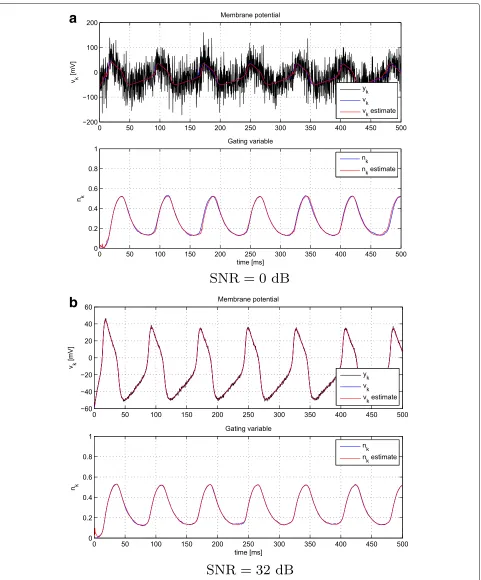
To give some intuition on the operation and perfor-mance of the PF method in Algorithm 1, we show the results for a single realization in Fig. 2. The results are for 500 particles and two different values ofσ_y2_,k, correspond-ing to 0 and 32 dB, respectively. Even in very low SNR regimes, the method is able to operate and provide reliable filtering results.

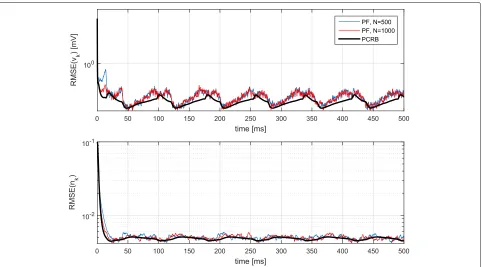
In order to evaluate the efficiency of the proposed esti-mation method, we computed the Posterior Cramér-Rao Bound (PCRB) [52] in Appendix 2. We plot the PCRB as a benchmark for the root mean square error (RMSE) curves obtained by computer simulations, obtained after aver-aging 200 independent Monte-Carlo trials. For a generic time serieswk, the RMSE of an estimatorwˆkis defined as tion andMthe number of independent Monte-Carlo trials used to approximate the mathematical expectation.

a

b

Fig. 2A single realization of the PF method foraSNR₌0 dB andbSNR₌32 dB

entire simulation time. The worst efficiency on estimat-ingvkwas 1.43 corresponding to 500 particles and 10% of inaccuracies (see Fig. 4), and the best was 1.11 for 1000

Fig. 3Evolution of the RMSE and the PCRB over time. Model inaccuracies where_σI=0.01·IoandσgL=0.01· ¯goL

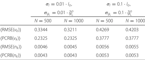
inaccuracies, the method seems more reactive. This is because the covariance associated with the state-space has larger values, resulting in a more nervous filter and, consequently, with smaller convergence rates. As a con-clusion, the PF tends to the PCRB with the number of particles. Also, the performance (both theoretical and empirical) could be improved if model inaccuracies are reduced, i.e., if the model parameters are better estimated at a previous stage. For the sake of completeness, we sum-marize the results in Table 1, where the average RMSE and PCRB along the 500-ms simulation are provided. It is apparent that increasing the number of particles from N = 500 toN =1000 does not improve significantly the performance of the method.

4.2 Model parameters are unknown

In this section, we validate the algorithm presented in Section 3.2. According to the previous analysis, we deem that 500 particles are enough for the filter to provide reli-able results. The parameters of the PMCMC algorithm were set toγ =0.9 andα¯∗=0.234.

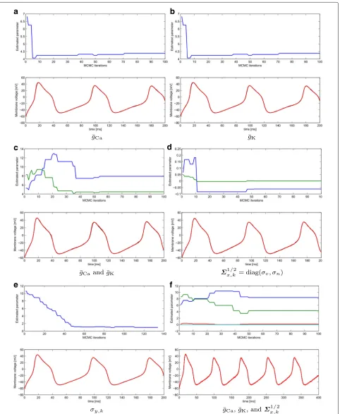
Figure 5 shows the results for a single realization when a number of parameters in the nominal model are unknown. We considered one, two, and four unknown parameters. Each of the plots includeM=100 iterations of the MCMC showing the evolution of the parameter estimation (top) and the superimposed recorded voltage in black and the filtered voltage trace in red (bottom). Model inaccuracies are of 1%, similarly as in Fig. 3. In these plots, we omitted the results for the gating vari-able for the sake of clarity. The true and initial values used in the experiments, as well as the initial covariances assumed, are detailed in Table 2. From the plots, we can observe that the method performs reasonably well even in the case of estimating the model parameters at the same time it is filtering out the noise in the membrane voltage traces.

A biologically meaningful signal is the leakage cur-rent. In general, the leakage gathers those ionic channels that are not explicitly modeled and other non-modeled sources of activity. The parameters driving the leak cur-rent areg¯LandEL. We tested and validated the proposed

Table 1Averaged results over simulation time

σI=0.01·Io, σI=0.1·Io,

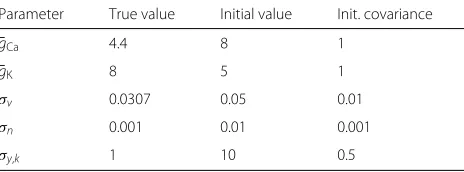
PMCMC in an experiment where the leak parameters were estimated at the same time the filtering solution was computed. Moreover, the statistics of the process noise were estimated as well, x,k. In this case, we iterated the PMCMC method 1000 times and average the results over 100 Monte-Carlo independent trials. The results are shown in Fig. 6, where the RMSE perfor-mance of the PMCMC method is compared to the per-formance of the original PF with perfect knowledge of the model.

It can be observed that the filtering performances with perfect knowledge of the model and with estimation of parameters by PMCMC are similar. Moreover, both approaches attain the theoretical lower bound of accuracy given by the PCRB, which is derived from the true model; see Appendix 2.

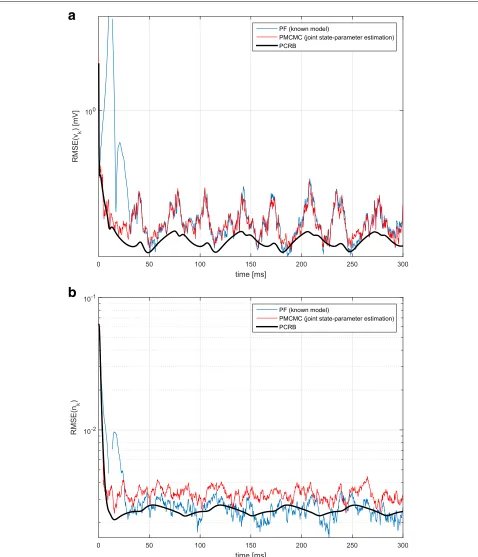
In Fig. 7, validation results for the parameter estima-tion capabilities of the PMCMC are shown. Particularly, we plotted a number of independent realizations of the

sample trajectories

θ(j)M

j=1. We observe that all of them converge to the true values of the parameter. Recall that these true values were θ = (g¯L,EL) = (2,−60). The average of these realizations is given in Fig. 7, where the aforementioned convergence to the true parameter is highlighted.

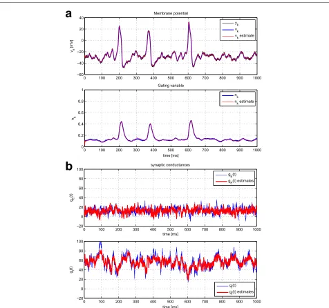
4.3 Estimation of synaptic conductances

Finally, once the methods to estimate state variables and unknown parameters were consolidated, we proceeded to test the methods to our ultimate goal: estimating jointly the intrinsic states of the neuron and the extrinsic inputs (i.e., the synaptic conductances).

First, the method with perfect knowledge of the model was validated in Fig. 8. It can be observed that the intrin-sic signals can be effectively recovered as before where synaptic inputs were not accounted for. The estimation of gE(t) andgI(t) is quite accurate, and the presence of spikes does not degrade the estimation capabilities of the method.

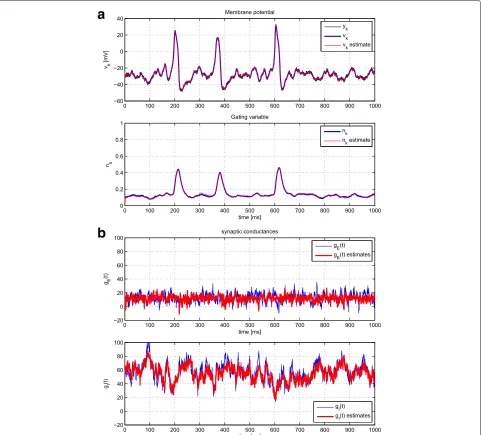
The PMCMC algorithm was tested similarly. In this case, we assumed that the model parameters related tovk andnk were accurately estimated, for instance, using an off-line procedure or that analyzed in Section 4.2. There-fore, we focused on the estimation of those parameters that describe the OU process of each of the synaptic terms. Particularly, we considered the values in Table 3. The results can be consulted in Fig. 9 and compared to those in Fig. 8.

a

c

d

b

e

f

Table 2True value, initial value, and covariance of the parameters in Fig. 5

Parameter True value Initial value Init. covariance

¯

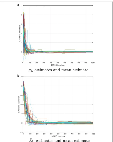
is normal since in this case a perfect knowledge of the model is assumed while the PMCMC needs to estimate both model parameters and synaptic conductances. More precisely, we have computed the normalized error

in both cases and obtained values of 0.2957 and 0.1939 for the excitatory and inhibitory conductances, respectively, with the PF method, and 0.3313 and 0.2095 (excitatory and inhibitory, respectively) with the PMCMC method. Compared to previous results in the literature, see, for instance, Figs. 2, 3, 4, 5, 6, and 8 in [4], where the authors performed an exhaustive comparison with different meth-ods, our estimations provide excellent agreement with the prescribed conductances. Moreover, our statistics include data obtained in the spiking regime while the methods compared in [4] are applied only to subthreshold voltage traces. We also observe that the errors for the PMCMC method are, in average, only 12% (excitatory) and 8% (inhibitory) worse than the errors for the PF method. Given the complexity of the PMCMC method, these find-ings encourage future applications of the method to exper-imental data even when the model is not well defined.

We refer to the Additional file 1 to visualize a dynamic simulation showing how the estimations evolve as the PMCMC algorithm was applied in a case where the values ofg¯LandELwere unknown.

5 Conclusions

In this paper, we propose a filtering method that is able to sequentially infer the time course of the membrane potential, the intrinsic activity of ionic channels, and the input synaptic conductances from noisy observations of voltage traces. The method works both for subthreshold and spiking regimes. It is based on the PF methodology

and features an optimal importance density, providing enhanced use of the particles that characterize the fil-tering distribution. In addition, we tackle the problem of joint parameter estimation and state filtering by extend-ing the designed PF with an MCMC procedure in an iterative method known as PMCMC. Another distinctive contribution with respect to the other works in the lit-erature is that here, we provide accuracy bounds for the problem at hand, given by the PCRB. The RMSEs of our methods are then compared to the bound, and therefore, we can assess the efficiency of the proposed inference methods.

Filtering methods of different types (e.g., PF or sigma-point Kalman filtering) have been used in other recent contributions to similar problems; see [7–13]. From a methodological perspective, the novelty of this paper is in the use of an optimal importance density to generate par-ticles, a fact that increases the estimation accuracy for a given budget of particles. This technical detail only applies to PF methods. Although Gaussian methods (e.g., the family of sigma-point Kalman filters) have a lower com-putational cost in general, they require Gaussianity of the measures, whereas PFs do not. This is an advantage that we think can be crucial in estimating synaptic conduc-tances, since the assumption of Gaussianity is generally assumed in the literature [4, 33], but there are no conclu-sive evidences to assert this assumption. In this paper, we have still applied the PF to an Ornstein-Uhlenbeck process in order to check that basic results can be attained, but further research will go in the direction of assuming other types of distributions for the synaptic conductances. The use of more complex distributions nicely fits within the framework of our PF-based method. Another advantage of PFs versus Gaussian filters is their enhanced robustness to outliers [53]; for instance, due to recording artifacts, future applications shall also incorporate this feature.

We have found excellent estimations of the synaptic conductances, even in spiking regimes. Estimating synap-tic conductances in spiking regimes is a challenge which is far to be solved. It is well known that linear esti-mations of synaptic conductances are not trustable in this situation when data is extracted intracellularly from the spiking activity of neurons; see [14]. In experiments, thus, caution has to be taken in eliminating part of the voltage traces, thus losing also part of the temporal infor-mation of both excitatory and inhibitory conductances. Our method is able to perform well in this regime. This information is highly valuable in problems (epilepsy, schizophrenia, Alzheimer’s disease, etc.) where a debate on the balance of excitation and inhibition is open; see the introduction of [12] for a rather complete overview on this feature.

a

b

Fig. 6Evolution ofaRMSE(vk) andbRMSE(nk) over time for the PMCMC method estimating the leakage parameters. Model inaccuracies where

a

b

Fig. 7Parameter estimation performance of the proposed PMCMC algorithm.aTop plot shows results forg¯L=2 estimation and (b) bottom plot

a

b

Fig. 8A single realization of the PF method with perfect model knowledge, estimating voltage, and gating variables (a) and synaptic conductances in nS (b). See Table 3 for the true value, initial value, and covariance of the parameters used here

Table 3True value, initial value, and covariance of the

parameters in Fig. 9

Parameter True value Initial value Init. covariance

τE 2.73 1.5 1

gE,0 12.1 10 1

σE 12 25 5

τI 10.49 15 10

gI,0 57.3 45 10

σI 26.4 35 5

a

b

Fig. 9A single realization of the PMCMC method, estimating voltage and gating variables (a) and synaptic conductances in nS (b) as well as model parameters. See Table 3 for the true value, initial value, and covariance of the parameters used here

parameters of the model and synaptic conductances. The latter problem is a challenging hot topic in the neuro-science literature, which is recently focusing on methods to extract the conductances from single-trace measure-ments. We think that our PF method would give useful and interesting results to physiologists that aim at infer-ring the brain’s activation rules from neurons’ activities. Actually, knowing the excitatory-inhibitory time-course separation can help in getting important conclusions about the brain’s functional connectivity (see [54–56]).

We have not tried to obtain estimations when sub-threshold ionic currents are active, where the presence

a

b

Fig. 10Comparison of estimated excitatory (a) and inhibitory (b) synaptic conductances versus the actual ones. We show both the performance of the PF method (round circles), which assumes a perfect knowledge of the model, and the PMCMC method (red dots)

Appendix 1: Morris-Lecar neuron model

From the myriad of existing single-neuron models, we consider without loss of generality the Morris-Lecar model proposed in [34]. The model can be related (see [36]) to the INa,p + IK model (persistent sodium plus potassium model). The dynamics of the neuron is mod-eled by a continuous-time dynamical system composed of the current-balance equation for the membrane potential, v = v(t), and the K+gating variable 0 ≤ n = n(t) ≤ 1,

which represents the probability of the K+ionic channel to be active. Then, the system of differential equations is

Cmv˙ = −IL−ICa−IK+Iapp (40)

˙

n = φn∞(v)−n

τn(v)

, (41)

in (40). The leakage, calcium, and potassium currents are librium potentials, for which the corresponding current is zero, a.k.a. reverse potentials.

The dynamics of the activation variable m is consid-ered at the steady state, and thus, we writem = m∞(v). On the other hand, the time constantτn(v)for the gating variable n cannot be considered that fast and the cor-responding differential equation needs to be considered. The formulae for these functions are

m∞(v) = 1

The knowledgeable reader would have noticed that the Morris-Lecar model is a Hodgin-Huxley-type model with the usual considerations, where the following two extra assumptions were made: the depolarizing current is gen-erated by Ca2+_{ionic channels (or Na}+_{depending on the} type of neuron modeled), whereas hyperpolarization is carried by K+ ions, and that m = m_∞(v). The Morris-Lecar model is very popular in computational neuro-science as it models a large variety of neural dynamics while its phase-plane analysis is more manageable as it involves only two states [35].

The Morris-Lecar, although simple to formulate, results in a very interesting model as it can produce a number of different dynamics. For instance, for given values of its parameters, we encounter a subcritical Hopf bifurcation forIapp =93.86μA/cm2. On the other hand, for another set of parameter values, the system of equations has a Saddle-Node on an Invariant Circle (SNIC) bifurcation at Iapp=39.96μA/cm2.

Appendix 2: PCRB in Morris-Lecar models

This appendix is devoted to the derivation of the PCRB estimation bound for the Morris-Lecar model used to benchmark the proposed methods in the simulations. We follow the sequential procedure given in [58], accounting that we have nonlinear functions in the state evolution and linear measurements, both with additive Gaussian

noise. We are interested in an estimation error bound of the type of Recall that the state-space we are dealing with is of the form

In this case, the PCRB can be computed recursively by virtue of the result in [58] by computing the following terms

D11_k = Exk

and plugging them into

Jk+1=D22_k −D21_k

Jk+D11_k −1

D12_k , (55)

for some initialJ0. Notice that, in our case,D22_k becomes deterministic, but the rest of the terms involving expec-tations should be computed by Monte-Carlo integration over independent state trajectories.

Since the state function is nonlinear, we use the Jacobian evaluated at the true value ofxkinstead, that is,

˜

where functionsf1andf2are as in (8) and (9), respectively. Therefore, to evaluate the bound, we need to compute the derivatives in the Jacobian. These are

with

Additional file 1:Evolution of the iterative learning when estimating leakage parameters. (MP4 2129 KB)

Funding

The work of the second author was supported by the project

MTM2015-71509-C2-2-R (MINECO/FEDER) and by the grant 2014-SGR-504 (Government of Catalonia).

Authors’ contributions

Both authors contributed equally to this work. Both authors read and approved the final manuscript.

Competing interests

The authors declare that they have no competing interests.

Publisher’s Note

Springer Nature remains neutral with regard to jurisdictional claims in published maps and institutional affiliations.

Author details

1_{Northeastern University, Boston, MA 02115, USA.}2_{Universitat Politècnica de}

Catalunya, 08028 Barcelona, Spain.

Received: 3 March 2017 Accepted: 18 August 2017

References

1. R Brette, A Destexhe,Handbook of neural activity measurement. (Cambridge University Press, New York, 2012). http://dx.doi.org/10.1017/ CBO9780511979958

2. QJM Huys, L Paninski, Smoothing of and parameter estimation from, noisy biophysical recordings. PLoS Comput. Biol.5(5), 1–16 (2009) 3. S Ditlevsen, A Samson, Estimation in the partially observed stochastic

Morris-Lecar neuronal model with particle filter and stochastic approximation methods. Ann. Appl. Stat.8(2), 674–702 (2014). doi:10.1214/14-AOAS729

4. M Lankarany, W-P Zhu, MNS Swamy, Joint estimation of states and parameters of Hodgkin-Huxley neuronal model using Kalman filtering. Neurocomputing.136, 289–299 (2014). http://dx.doi.org/10.1016/j. neucom.2014.01.003

5. S Ditlevsen, A Samson, Parameter estimation in neuronal stochastic differential equation models from intracellular recordings of membrane potentials in single neurons: a review. J. de la Socié.157(1), 6–16 (2016) 6. Y Mishchenko, JT Vogelstein, L Paninski, A Bayesian approach for inferring

neuronal connectivity from calcium fluorescent imaging data. Ann. Appl. Stat.5(2B), 1229–1261 (2011). doi:10.1214/09-AOAS303. http://dx.doi.org/ 10.1214/09-AOAS303

7. M Rudolph, Z Piwkowska, M Badoual, T Bal, A Destexhe, A method to estimate synaptic conductances from membrane potential fluctuations. J. Neurophysiol.91(6), 2884–2896 (2004). doi:10.1152/jn.01223.2003. jn. physiology.org/content/91/6/2884.full

8. M Pospischil, M Toledo-Rodriguez, C Monier, Z Piwkowska, Thierry Bal, Y Frégnac, H Markram, A Destexhe, Minimal Hodgkin-Huxley type models

for different classes of cortical and thalamic neurons. Biol. Cybernet.

99(4-5), 427–441 (2008)

9. C Bédard, S Béhuret, C Deleuze, T Bal, A Destexhe, Oversampling method to extract excitatory and inhibitory conductances from single-trial membrane potential recordings. J. Neurosci. Methods (2011). doi:10.1016/j.jneumeth.2011.09.010

10. R Kobayashi, Y Tsubo, P Lansky, S Shinomoto, Estimating time-varying input signals and ion channel states from a single voltage trace of a neuron. Adv. Neural Inf. Process. Syst. (NIPS).24, 217–225 (2011) 11. L Paninski, M Vidne, B DePasquale, DG Ferreira, Inferring synaptic inputs

given a noisy voltage trace via sequential Monte Carlo methods. J. Comput. Neurosci.33(1), 1–19 (2012)

12. RW Berg, S Ditlevsen, Synaptic inhibition and excitation estimated via the time constant of membrane potential fluctuations. J. Neurophysiol.

110(4), 1021–1034 (2013). doi:10.1152/jn.00006.2013

13. M Lankarany, WP Zhu, MNS Swamy, T Toyoizumi, Inferring trial-to-trial excitatory and inhibitory synaptic inputs from membrane potential using Gaussian mixture Kalman filtering. Front. Comput. Neurosci.7(2013). doi:10.3389/fncom.2013.00109. http://dx.doi.org/10.3389/fncom.2013. 00109

14. A Guillamon, DW McLaughlin, J Rinzel, Estimation of synaptic conductances. J. Physiology-Paris.100(1-3), 31–42 (2006). doi:10.1016/j.jphysparis.2006.09.010

15. C Vich, A Guillamon, Dissecting estimation of conductances in subthreshold regimes. J. Comput. Neurosci, 1–17 (2015). doi:10.1007/s10827-015-0576-2

16. P Closas, A Guillamon, inProceedings of the IEEE International Conference on Acoustics, Speech, and Signal Processing, ICASSP 2013. Sequential estimation of gating variables from voltage traces in single-neuron models by particle filtering, (Vancouver, 2013)

17. P Closas, A Guillamon, Estimation of neural voltage traces and associated variables in uncertain models. BMC Neurosci.14(1), 1151 (2013) 18. A Doucet, N de Freitas, N Gordon,Sequential Monte Carlo methods in

practice. (Springer, 2001)

19. PM Djuric, SJ Goodsill, Guest editorial special issue on Monte Carlo methods for statistical signal processing. Signal Process. IEEE Trans.50(2), 173–173 (2002). doi:10.1109/TSP.2002.978373

20. PM Djuri´c, JH Kotecha, J Zhang, Y Huang, T Ghirmai, MF Bugallo, J Míguez, Particle filtering. IEEE Signal Process. Mag.20(5), 19–38 (2003)

21. S Arulampalam, S Maskell, N Gordon, T Clapp, A tutorial on particle filters for online nonlinear/non-Gaussian Bayesian tracking. IEEE Trans. Signal Process.50(2), 174–188 (2002)

22. Z Chen, Bayesian filtering: from Kalman filters to particle filters, and beyond. Technical report, Adaptive Syst. Lab., McMaster University, Ontario, Canada (2003)

23. B Ristic, S Arulampalam, N Gordon,Beyond the Kalman filter: particle filters for tracking applications. (Artech House, Boston, 2004)

24. S Särkkä,Bayesian filtering and smoothing. (Cambridge University Press, New York, 2013)

25. A Doucet, SJ Godsill, C Andrieu, On sequential Monte Carlo sampling methods for Bayesian filtering. Stat. Comput.3, 197–208 (2000) 26. DV Vavoulis, VA Straub, JAD Aston, J Feng, A self-organizing

state-space-model approach for parameter estimation in Hodgkin-Huxley-type models of single neurons. PLoS Comput. Biol.8(3) (2012). e1002401 27. G Ullah, SJ Schiff, Tracking and control of neuronal Hodgkin-Huxley

dynamics. Phys. Rev. E.79(4), 040901 (2009)

28. CM Carvalho, MS Johannes, HF Lopes, NG Polson, et al., Particle learning and smoothing. Stat. Sci.25(1), 88–106 (2010)

29. N Chopin, PE Jacob, O Papaspiliopoulos, SMC2: an efficient algorithm for sequential analysis of state space models. J. R. Stat. Soc. Series B (Stat. Methodol.)75(3), 397–426 (2013)

30. CC Drovandi, JM McGree, AN Pettitt, A sequential Monte Carlo algorithm to incorporate model uncertainty in Bayesian sequential design. J. Comput. Graphical Stat.23(1), 3–24 (2014)

31. I Urteaga, MF Bugallo, PM Djuri´c, inStatistical Signal Processing Workshop (SSP) 2016 IEEE. Sequential Monte Carlo methods under model uncertainty (IEEE, Mallorca, 2016), pp. 1–5

33. M Rudolph, A Destexhe, Characterization of subthreshold voltage fluctuations in neuronal membranes. Neural Comput.15(11), 2577–2618 (2003) 34. C Morris, H Lecar, Voltage oscillations in the barnacle giant muscle fiber.

Biophys J.35(1), 193–213 (1981)

35. JR Rinzel, GB Ermentrout, inMethods in neural modeling, ed. by C Koch, I Segev. Analysis of neural excitability and oscillations (MIT Press, Cambridge, 1998), pp. 135–169

36. E Izhikevich,Dynamical systems in neuroscience: the geometry of excitability and bursting. (MIT Press, Cambridge, 2006)

37. R Douc, O Cappé, E Moulines, inProc. of the 4th International Symposium on Image and Signal Processing and Analysis, ISPA’05. Comparison of resampling schemes for particle filtering, (Zagreb, 2005), pp. 64–69 38. C Andrieu, A Doucet, SS Singh, VB Tadic, Particle methods for change

detection, system identification, and control. Proc. IEEE.92(3), 423–438 (2004) 39. C Andrieu, A Doucet, VB Tadic, inDecision and Control 2005 and 2005

European Control Conference.CDC-ECC ’05. 44th IEEE Conference on. On-line parameter estimation in general state-space models, (Seville, 2005), pp. 332–337

40. G Poyiadjis, A Doucet, SS Singh, Particle approximations of the score and observed information matrix in state space models with application to parameter estimation. Biometrika.98, 65–80 (2011)

41. C Andrieu, A Doucet, R Holenstein, Particle Markov Chain Monte Carlo methods. J. R. Stat. Soc. Series B.72(3), 269–342 (2010)

42. L Martino, V Elvira, G Camps-Valls, Group importance sampling for particle filtering and MCMC (2017). arXiv preprint arXiv:1704.02771

43. WR Gilks, S Richardson, DJ Spiegelhalter,Markov Chain Monte Carlo in practice: interdisciplinary statistics. CRC Interdisciplinary Statistics Series. (Chapman & Hall, 1996)

44. C Berzuini, N Best, W Gilks, C Larizza, Dynamic conditional independence models and Markov Chain Monte Carlo methods. J. Am. Stat. Assoc.92, 1403–1412 (1997)

45. JS Liu. Monte Carlo strategies in scientific computing (Springer, New York, 2008)

46. S Brooks, A Gelman, G Jones, X-L Meng,Handbook of Markov Chain Monte Carlo. (CRC Press, Boca Raton, 2011)

47. S Donnet, A Samson, Using PMCMC in EM algorithm for stochastic mixed models: theoretical and practical issues. J. Soc. Franç, aise de Statistique.

155(1), 49–72 (2014)

48. M Vihola, Robust adaptive metropolis algorithm with coerced acceptance rate. Stat. Comput.22(5), 997–1008 (2012)

49. H Haario, E Saksman, J Tamminen, et al., An adaptive metropolis algorithm. Bernoulli.7(2), 223–242 (2001)

50. D Luengo, L Martino, inAcoustics, Speech and Signal Processing (ICASSP) 2013 IEEE International Conference on. Fully adaptive Gaussian mixture Metropolis-Hastings algorithm (IEEE, 2013), pp. 6148–6152

51. GH Golub, CF van Loan,Matrix computations, 3edition. (The John Hopkins University Press, Baltimore, 1996)

52. HL Van Trees, KL Bell,Bayesian bounds for parameter estimation and nonlinear filtering/tracking. (Wiley Interscience, Piscataway, 2007) 53. PM Djuri´c, MF Bugallo, P Closas, J Míguez, inProceedings of the IEEE

International Workshop on Computational Advances in Multi-Sensor Adaptive Processing, CAMSAP’09. Measuring the robustness of sequential methods (Dutch Antilles, 2009)

54. JS Anderson, M Carandini, D Ferster, Orientation tuning of input conductance, excitation, and inhibition in cat primary visual cortex. J. Neurophysiol.84(2), 909–926 (2000). jn.physiology.org/content/84/2/ 909.short

55. M Wehr, AM Zador, Balanced inhibition underlies tuning and sharpens spike timing in auditory cortex. Nature.426(6965), 442–446 (2003). doi:10.1038/nature02116. http://dx.doi.org/10.1038/nature02116 56. C Bennett, S Arroyo, S Hestrin, Subthreshold mechanisms underlying

state-dependent modulation of visual responses. Neuron.80(2), 350–357 (2013). http://dx.doi.org/10.1016/j.neuron.2013.08.007

57. SJ Cox, Estimating the location and time course of synaptic input from multi-site potential recordings. J. Comput. Neurosci.17, 225–243 (2004) 58. P Tichavský, CH Muravchik, A Nehorai, Posterior Cramér-Rao bounds for