R E S E A R C H
Open Access
GNSS-based bistatic SAR: a signal processing view
Michail Antoniou
*and Mikhail Cherniakov
Abstract
This article presents signal processing algorithms used as a new remote sensing tool, that is passive bistatic SAR with navigation satellites (e.g. GPS, GLONASS or Galileo) as transmitters of opportunity. Signal synchronisation and image formation algorithms are described for two system variants: one where the receiver is moving and one where it is fixed on the ground. The applicability and functionality of the algorithms described is demonstrated through experimental imagery that ultimately confirms the feasibility of the overall technology.
Keywords:bistatic SAR signal processing, SS-BSAR, GNSS-based SAR
1. Introduction
Over the last decade, bistatic SAR (BSAR) has seen a substantial growth. Various BSAR topologies have been proposed, using spaceborne, airborne or even fixed plat-forms [1-4], and their relative merits and drawbacks have been investigated.
A special BSAR topology is called space-surface BSAR (SS-BSAR), or hybrid BSAR [5]. In this configuration, one of the platforms is spaceborne, while the other is located on or near the surface of the Earth (Figure 1). Even though this topology is a special BSAR case, it encompasses a variety of possible transmitter/receiver combinations. The transmitter could be spaceborne, while the receiver could be mounted on an aircraft, a ground moving vehicle, or it could be fixed on the ground, or vice versa. The only requirement is that at least one platform should move relative to an observa-tion area, such that a synthetic aperture can be formed. The spaceborne platform can be a radar satellite [6-8], which is the most common case. Alternatively, it can be a transmitter of opportunity, such as a communications or digital television satellite.
Our research focuses on SS-BSAR using global naviga-tion satellite systems (GNSS) as transmitters of oppor-tunity [9-13]. There are a number of reasons for this choice. First of all, GNSS are satellite constellations consisting of at least 24 satellites, and are designed for global and permanent coverage. From the radar perspec-tive, this enables persistent area monitoring. In addition,
GNSS are designed in such a way that there are at least six to eight satellites illuminating the same point on Earth from multiple angles. This enables simultaneous image acquisition from multiple angles which may pro-vide further scene information. The presence of multiple satellites also provides the possibility to choose the optimal bistatic acquisition geometry, minimising sha-dowing effects due to local landscape and maximising resolution performance.
In terms of the passive operation, use of GNSS is an ideal choice. First of all, GNSS exhibit relatively large sig-nal bandwidths compared to other sources of opportun-ity, and can therefore provide sufficient range resolutions (the aggregate signal bandwidth for the Galileo E5 band is approximately 20 MHz). More importantly, however, the receiving hardware for SS-BSAR is very similar, if not identical, to a standard GPS receiver used for navigation purposes. On one hand, this implies that SS-BSAR based on GNSS is cost-effective, as standard GPS chipsets can nowadays be purchased at extremely low costs.
On the other hand, this implies that changing the signal processing algorithms within the standard GPS chipset can convert the device into a low-cost radar system, with all the advantages mentioned above. This raises the question of which signal processing algorithms can be used in this system.
All BSAR systems require two types of algorithms to provide imagery. The first type is signal synchronisation, aiming to maintain coherence for image formation. This step is necessary, since the transmitter and receiver are separated, and hence have independent clocks and local
oscillators. To provide synchronisation, an extra
* Correspondence:[email protected]
School of Electronic, Electrical and Computer Engineering, University of Birmingham, Edgbaston, Birmingham B15 2TT, UK
receiving channel is usually added, which records the dir-ect signal from the transmitter to the receiver. Extraction and analysis of the parameters of the direct signal, such as delay and phase, is sufficient to provide the necessary delay and phase references required for imaging. In trad-itional BSAR, where the transmitter is a radar platform, the transmitted power is high and the transmitted signal is a chirp waveform. In this case, a number of solutions have been proposed [14,15]. In SS-BSAR with GNSS, none of the traditional solutions are applicable and signal synchronisation is a complex issue. The reason for that is that GNSS signals have a low power density near the sur-face of the Earth, resulting in signal-to-noise ratios (SNR) of down to−40 dB at the receiver input [16]. The other reason is that GNSS are communication signals with complex modulation schemes which should be cancelled before extraction of direct signal parameters.
The second type of algorithms required is of course image formation algorithms. The derivation of image for-mation algorithms has been a major challenge in BSAR since its conception. There are a number of image forma-tion algorithms operating in the frequency domain for
special BSAR topologies, such as parallel/linear transmitter and receiver trajectories or equal platform velocities [17-20]. Fast back-projection algorithms (BPAs) have been proposed for the general BSAR case [21]. However, to the best of the authors’ knowledge, a generic closed-form solution for a frequency-based algorithm without any ap-proximation is yet to be presented. The reason behind this is that the different transmitter/receiver trajectories result in azimuth signals which are difficult to convert to the frequency domain analytically. This problem is more acute for SS-BSAR. A satellite and an aircraft cannot follow paral-lel trajectories, nor have equal velocities. Moreover, in the moving receiver case, a suitable motion compensation algorithm is required to correct for trajectory deviations of the aircraft only.
This article describes signal synchronisation and image formation algorithms employed in SS-BSAR with GNSS transmitters of opportunity. The functionality of the algo-rithms, and ultimately the proposed technology, is demon-strated using a variety of experimental data, obtained from both moving receivers (roof top railways, ground moving vehicle and a helicopter) as well as a stationary one. Sec-tion 2 presents an overview of the signal synchronisaSec-tion al-gorithm used, along with experimental results. Section 3 describes image formation algorithms developed for the moving and stationary receiver cases. Finally, Section 4 pre-sents experimental imagery using the configurations de-scribed above.
2. Signal synchronisation 2.1. Introduction
Whether the receiver is stationary or not, SS-BSAR with GNSS uses one receiving channel to record the direct sig-nal from the satellite for synchronisation, while another channel collects satellite signal reflections from an observa-tion area for imaging. The direct signal channel is called the heterodyne channel (HC), and the reflected signal channel is called the radar channel (RC). Both the HC and
Figure 1SS-BSAR concept.
RC have the same clocks and local oscillators, and there-fore clock slippage and local oscillator drift between the transmitter and the receiver is common to both channels. As a result, clock slippage and oscillator drift can be deducted through the delay and phase of the direct signal at the HC and then compensated at the RC.
The reason for having the HC is that an antenna can be pointed towards the satellite to maximise the direct signal strength. Even in this case, the SNR at the input of the re-ceiver can be as low as−40 dB, so the HC signal cannot be used for synchronisation directly. This implies that in order to estimate the direct signal delay and phase, and extract from them the required clock slippage and oscillator drift, a tracking algorithm based on matched filtering is required to maximise SNR. An additional problem is the structure of all GNSS signals. They are communication signals consisting of two ranging codes which are pseudorandom sequences, which generally (but not necessarily) modulate a navigation message. From these three sequences, only the primary ranging code is desired as the transmitted sig-nal for imaging, while the other two act as interference. Hence, a method of tracking the parameters of the primary code and cancelling the interfering codes is required.
2.2. Synchronisation algorithm description
One possible method of providing signal synchronisation for SS-BSAR with GNSS is to modify signal processing al-gorithms used for GNSS signal tracking for navigation pur-poses. The purpose of this class of algorithms is to cancel all ranging codes and extract the navigation message re-quired for positioning. However, in order to do so, they need to track the time delay, Doppler and phase of the ran-ging codes. In SS-BSAR with GNSS, the ranran-ging code is the transmitted signal and hence its tracked parameters on the HC are the required synchronisation outputs.
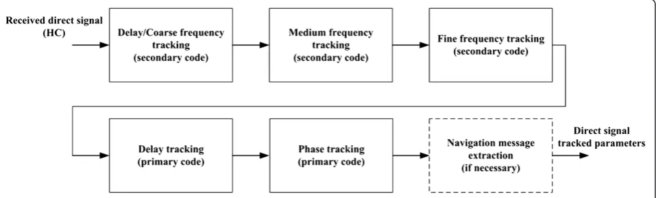
The particular algorithm adapted from GNSS signal tracking to SS-BSAR synchronisation is the well-known block adjustment of synchronising signal (BASS) algorithm [22]. Its block diagram for signal synchronisation is shown in Figure 2.
An algorithm for SS-BSAR signal synchronisation based on this technique was proposed at the first devel-opment stages of the system [23]. While highly accurate, it did not meet efficiency requirements, and therefore it was replaced by the algorithm described below. The ge-neric form of a transmitted GNSS signal is:
Y tð Þ ¼P tð ÞMPð Þt cosðωctþφÞ
þD tð ÞMDð Þt sinðωctþφÞ; ð1Þ
where t is time, P(t) and D(t) are the primary and sec-ondary GNSS ranging code envelopes, Mp(t) andMD(t)
are the associated navigation messages, ωc is the signal carrier frequency andφis the initial signal phase.
After quadrature demodulation and SAR data format-ting, the direct signal received at the HC can be written as follows:
stantaneous direct signal time delay, Doppler and initial phase associated with each code, respectively, all of which are varying with slow-time. Note that the primary and sec-ondary codes are different in structure and length, and therefore their time delays and phases are different by a constant value. However, their Doppler, defined as the de-rivative of their phases, are approximately equal.
As mentioned before, the signal required for SS-BSAR image formation is the primary code P(t), and hence all of its parameters should be tracked for synchronisation. However, according to (2), the secondary code D(t) is acting as a deterministic interference. The BASS algo-rithm first tracks the secondary code parameters prior to its compensation, and then proceeds to track the re-quired parameters of the primary code.
The first stage in the algorithm combines the delay τdD (u) and coarse Doppler frequency tracking of the second-ary code. These parameters are provided at every PRI, which for GNSS is usually 1 ms, resulting in a pulse repeti-tion frequency (PRF) of 1 kHz. The tracking process con-sists of a bank of matched filters. The envelope of each filter is a locally generated replica ofD(t), modulated with a different Doppler frequency. The Doppler separation be-tween filters is equal to the PRF (1 kHz), varied
incremen-tally between −20 and 20 kHz which is the maximum
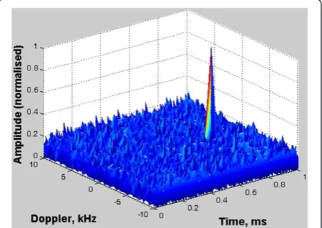
Doppler expected from a GNSS satellite [22]. Therefore, this stage is a 2D search algorithm in delay and Doppler, with a Doppler resolution of 1 kHz, hence the term“coarse frequency”. Figure 3 shows this processing step for a single Doppler frequency,ωdi, and Figure 4 presents a typical 2D delay/coarse frequency estimate for one PRI, obtained from experimental data. The location of the peak indicates the estimated delay and coarse frequency.
of the secondary code. This is achieved by stripping D[tn−τdD(u)] from the data (Figure 5).
At the output of the fine frequency tracking, the direct signal Dopplerωd(u) has been estimated. Even though it has been estimated using the secondary code, we may assume that it is the same for the primary code for the reasons described above.
Following the fine frequency tracking, the time delay and Doppler ofD(t) are known. Therefore, the secondary code with its parameters can be removed from (2). Note that the navigation messageMD(t) has not been tracked; however,
it can be viewed as a random signal with low cross-correlation values with the primary code and therefore can be neglected. With this observation, the second term in (2) is compensated and the remaining received signal may be written as follows:
s tðn;uÞ ¼P t½n−τdPð Þu MP½tn−τdPð Þuexp½jðωdð Þtu nþφdPð Þu Þ ð3Þ
In order to track τdP(u), matched filtering is used. The reference signal is the envelope ofP(t), shifted in Doppler byωd(u) which was estimated in the previous step. Finally, the phase and the navigation message (if one exists) can be extracted after the time-delayed and Doppler shifted
primary code have been stripped from (3), as shown in Figure 6. The navigation message is a BPSK signal, and can be regarded as a phase transition of ±π onφdP(u).
There-fore, using a phase transition detector, both the navigation message and the phase can be found.
At the output of the signal synchronisation algorithm, the direct signal time delay τdP(u), Doppler ωd(u), phase φdP(u) and navigation message Md(t) have been
esti-mated. In the following section, the derived algorithm is confirmed using various experimental data.
2.3. Experimental confirmation
The proposed algorithm was tested using two sets of ex-perimental data. The first set was obtained using a GLONASS transmitter and a fixed receiver, and the sec-ond was obtained with a Galileo transmitter and an air-borne receiver. These variants were selected to test the validity of the algorithm, as well as its functionality for different configurations and topologies.
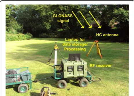
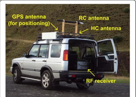
2.3.1. GLONASS transmitter and fixed receiver
A data acquisition dedicated to the verification of the synchronisation algorithm was conducted with a GLONASS transmitter and a fixed receiver (Figure 7). The direct signal from the satellite was captured by a stationary low-gain antenna, and the synchronisation al-gorithm was applied to extract its delay, Doppler, phase
Figure 3Delay/coarse frequency tracking block diagram.
Figure 4Output of delay/coarse frequency tracker for 1-ms data.
Input signal
PRN code
Output signal
and navigation message. The experimental parameters are shown in Table 1.
The primary GLONASS code is the P-code, while the C/A-code is the secondary, or interfering code. Figure 8a shows the tracked P-code delay, while Figure 8b presents the Doppler frequency at the output of the fine frequency tracker. Note that in practice, a least-mean squares algo-rithm is applied to the tracking output to smooth Doppler variation due to receiver noise. However, both delay and Doppler outputs are clear and without signifi-cant errors.
The tracked phase spectrum is shown in Figure 8c. This result was generated by taking the complex expo-nential of the tracked phase, followed by an FFT. Effect-ively, this is the azimuth spectrum of the direct signal. The obtained results shows a near-perfect chirp signal spectrum, which is as expected from the instantaneous phase history of the satellite. Finally, Figure 8d presents the decoded navigation message in the first 5 s of the data for better visualisation.
The results presented in Figure 8 demonstrate the func-tionality and high performance level of the proposed method. Note that the tracked outputs contain both the true time delay and Doppler variation, as well as receiver artefacts such as clock slippage and local oscillator drift. In the next chapter, methods of cancelling them out for effect-ive image formation will be described.
2.3.2. Galileo transmitter and airborne receiver
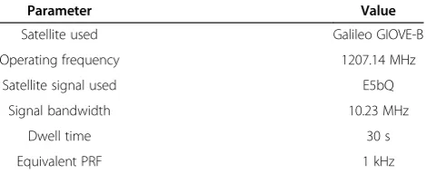
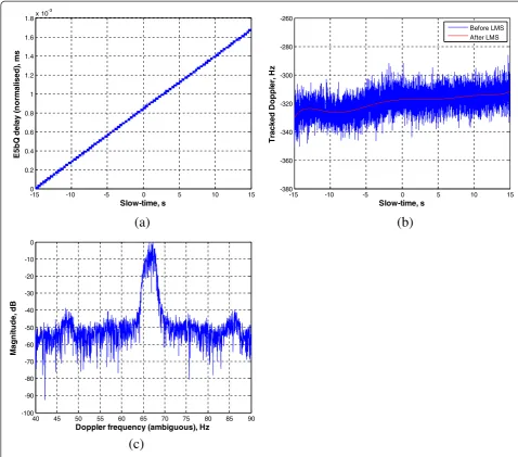
Experiments with a Galileo transmitter and an airborne re-ceiver were conducted in order to verify the imaging cap-ability of the system. The imaging experiment will be described in more detail in Section 3. Prior to image forma-tion, signal synchronisation was required. Experimental pa-rameters related to synchronisation are shown in Table 2. The difference in this case was that the HC was onboard the helicopter, and therefore the direct signal delay and Doppler variations were much more dynamic and affected by receiver motion errors. The Galileo E5bQ signal was used for imaging, which is free of a navigation message, and therefore navigation message extraction was not required.
Figure 9 shows the tracked direct signal parameters. Comparing Figures 9 and 8, it is clear that the direct signal Doppler in the moving receiver case is influenced by the trajectory deviations of the helicopter during its flight. The same effect is also visible in the tracked azi-muth phase spectrum, which is no longer representative of a chirp signal (Figure 9c).
A number of conclusions can be derived from the experimental results in this section. First of all, the pro-posed algorithm can operate irrespective of the GNSS transmitter used, and irrespective of the topology, even in a dynamic environment such as an airborne receiver where trajectory deviations affect the direct signal parame-ters. In terms of the performance, all tracked outputs are obtained with sufficiently high SNR. In the fixed receiver case, the tracked Doppler curve is linear, implying a stable signal Doppler history that resembles a chirp signal. In the moving receiver case, effects of trajectory deviations are
Figure 6Phase/navigation message extraction.
Figure 7SS-BSAR experimental setup with fixed receiver for synchronisation testing.
Table 1 Experimental parameters
Parameter Value
Satellite used GLONASS COSMOS 732
Operating frequency 1603.6875 MHz (L1)
Satellite signal used P-code
Signal bandwidth 5.11 MHz
Dwell time 300 s
Satellite elevation 48°–52°
Satellite azimuth 298°–301°
visible, an issue which should be dealt with at the image formation stage.
3. Image formation
Following signal synchronisation, an image formation al-gorithm is required to generate imagery of an interro-gated scene. In the general BSAR case, image formation algorithms need to take two things into account. The first is the outputs of the synchronisation algorithm to maintain coherence, and the second is the topology of the bistatic acquisition. The reason for the latter is that different acquisition geometries imply different bistatic range/Doppler histories, which may or may not allow ef-ficient processing algorithms in the frequency domain. This is particularly true for the SS-BSAR case, where there is little control in the choice of acquisition geom-etry due to the spaceborne transmitter. Another factor
to consider is the receiver configuration. A fixed receiver on the ground may generally be simpler in terms of the processing; however, this is not necessarily the case. On the other hand, a moving receiver has the added com-plexity of motion compensation.
(a)
(b)
(c)
(d)
-150 -100 -50 0 50 100 150
0 0.05 0.1 0.15 0.2 0.25
Slow-time, s
P-code delay (normalised), ms
-150 -100 -50 0 50 100 150
-1400 -1350 -1300 -1250 -1200 -1150 -1100
Slow-time, s
Tracked Doppler, Hz
Before LMS After LMS
0 100 200 300 400 500 600 700 800 900 1000
-80 -70 -60 -50 -40 -30 -20 -10 0
Doppler frequency (ambiguous), Hz
Magnitude, dB
-149.5 -149 -148.5 -148 -147.5 -147 -146.5 -146 -145.5 -145
-2 -1.5 -1 -0.5 0 0.5 1 1.5 2
Slow-time, s
Amplitude (normalised)
Figure 8Tracked direct signal: (a)delay,(b)Doppler,(c)phase spectrum,(d)decoded navigation message.
Table 2 Airborne experiment parameters related to synchronisation
Parameter Value
Satellite used Galileo GIOVE-B
Operating frequency 1207.14 MHz
Satellite signal used E5bQ
Signal bandwidth 10.23 MHz
Dwell time 30 s
For SS-BSAR with GNSS transmitters, one of the re-quirements was system operation independent of the acquisition geometry for the airborne receiver case. To accomplish this task, a range-Doppler algorithm with built-in motion compensation was originally built for this specific topology. This algorithm was tested on both simulated and experimental data under various geom-etries, and its full details can be found in [13,24].
However, due to the complexity of the algorithm, the requirement for system operation with both stationary and moving receivers, and the fact that the overall system study was at the proof-of-concept stage, a sim-pler bistatic BPA was built for global operation. In the next sections, the details of the algorithm will be pro-vided for the moving and stationary receiver cases.
3.1. BPA for GNSS-based SAR with a moving receiver
A three-dimensional GNSS-based SAR geometric model operating in strip map mode with a moving receiver is shown in Figure 10. The receiver could be airborne or a ground moving vehicle simply by adjusting the receiver altitude.
The coordinate system obeys the right-hand rule. The receiver moves along the y-axis and for simplicity, but without loss of generality, operates in broadside mode. This axis represents cross-range (y), and is linearly related to slow-time u by the speed of the receiver VR.
The x- and z-axes represent ground range and height, respectively. The origin of the coordinate system is the nadir of the midpoint of the synthetic aperture of the receiver. In the absence of motion errors, the
(a)
(b)
instantaneous coordinates of the SAR platform are given by (0,y(u),h), wherehis the receiver altitude and y(u) = VRU. If motion errors are present, the platform is shifted
from its nominal coordinates. In the airborne case, this could be due to atmospheric turbulence during flight, whereas in the ground moving vehicle case, these errors may refer to road anomalies. As a result, the true coordi-nates of the platform are given by (xe(u), ye(u), ze(u)).
The totality of across- and along-track errors will be re-ferred to as motion errors hereafter. The satellite is as-sumed to fly in a straight line, which is approximately true for a relatively short observation time. Its instantan-eous co-ordinates are given by (xT(u),yT(u),zT(u)).
Both the HC and RC are onboard the receiver. The in-stantaneous range from the transmitter to the receiver is the transmitter–receiver baseline, and given by
RBð Þ ¼u
ffiffiffiffiffiffiffiffiffiffiffiffiffiffiffiffiffiffiffiffiffiffiffiffiffiffiffiffiffiffiffiffiffiffiffiffiffiffiffiffiffiffiffiffiffiffiffiffiffiffiffiffiffiffiffiffiffiffiffiffiffiffiffiffiffiffiffiffiffiffiffiffiffiffiffiffiffiffiffiffiffiffiffiffiffiffiffiffiffiffiffiffiffiffiffiffiffiffi
xTð Þ−xu eð Þu
½ 2
þ½yTð Þ−yu eð Þu2þ½zTð Þ−zu eð Þu2
q
ð4Þ
On the other hand, for a point target located at co-ordinates (xTa, yTa, zTa), the instantaneous
transmitter-target and receiver-transmitter-target ranges RT(u) and RR(u) are
equal to
RTð Þ ¼u
ffiffiffiffiffiffiffiffiffiffiffiffiffiffiffiffiffiffiffiffiffiffiffiffiffiffiffiffiffiffiffiffiffiffiffiffiffiffiffiffiffiffiffiffiffiffiffiffiffiffiffiffiffiffiffiffiffiffiffiffiffiffiffiffiffiffiffiffiffiffiffiffiffiffiffiffiffiffiffiffiffiffiffiffiffiffiffi
xTð Þu −xTa
½ 2þ
yTð Þu −yTa
½ 2þ
zTð Þu −zTa
½ 2
q
ð5Þ
RRð Þ ¼u
ffiffiffiffiffiffiffiffiffiffiffiffiffiffiffiffiffiffiffiffiffiffiffiffiffiffiffiffiffiffiffiffiffiffiffiffiffiffiffiffiffiffiffiffiffiffiffiffiffiffiffiffiffiffiffiffiffiffiffiffiffiffiffiffiffiffiffiffiffiffiffiffiffiffiffiffiffiffiffiffiffiffiffiffi
xeð Þu −xTa
½ 2þ
yeð Þu −yTa
½ 2þ
zeð Þu −zTa
½ 2
q
ð6Þ
The HC records the direct signal, with a time delay and phase related toRB(u). The RC records the reflected
signal from the point target, with a time delay and phase related to the sumRT(u) andRR(u). However, all of these
parameters are severely affected by external, time vary-ing factors which make image focusvary-ing impossible with-out their compensation. These are related with time delay and phase errors due to receiver artefacts, denoted by teRx;φeRx such as clock slippage and local oscillator drift, as well as errors due to atmospheric propagation, teatm;φeatm. In the presence of these errors, the direct and
reflected signals at the HC and RC may be written as
where p(t) is the transmitted signal envelope (the pri-mary GNSS code in this case),cis the speed of light and
λis the radar wavelength.
Inspection of (7) and (8) shows that the HC and RC have been modelled as having the same errors. That is due to the fact that they are identical channels of the same receiver, and therefore they share common receiver errors and approximately equal atmospheric errors. Therefore, errors tracked during the HC synchronisation can be used to compensate errors in the RC.
An additional problem for image formation is the trajec-tory deviations of the receiver. In traditional monostatic SAR, where the same platform is used for signal transmis-sion and echo reception, motion compensation (MoComp) deals with the correction of trajectory deviations and is a well-known problem. In SS-BSAR, the situation is quite different. MoComp is required due to trajectory deviations of the receiving platform only, but the range and phase his-tory of the signal are composed of the sum of the transmitter-target and receiver-target ranges.
A block diagram of a BPA built to tackle all the prob-lems mentioned above is shown in Figure 11.
The BPA consists of two major steps in general: range compression and the calculation of the back-projection
integral. For the GNSS-based SAR case, the major pecu-liarity lies in the generation of the reference signal for range compression, and correction factors for MoComp.
The signal synchronisation algorithm tracks the direct signal time delay and phase, that is RBð Þu
c þteRxþteatm and 2π
λ RBð Þ þu φeRxþφeatm. In order to compensate for receiver
and atmospheric errors, it is necessary to separate them from the terms associated with the baseline lengthRB(u).
This is possible if the transmitter and receiver co-ordinates are known. That way, terms associated withRB(u) can be
calculated based on (4) and then removed from the syn-chronisation outputs. As soon as these errors are isolated, a reference signal for range compression may be written as follows:
s0ðt;uÞ ¼p t½ −ðteRxþteatmÞexp −j φeRxþφeatm
ð9Þ
Note that all the receiver and atmospheric errors change with slow-timeu, but are not direct functions of this parameter.
Range compression can be conducted in the fast-time frequency domain via an FFT on (8) and (9), complex con-jugate multiplication and an inverse FFT. At the output of this operation, the range-compressed RC data may be modelled as follows:
where Rx(t) is the cross-correlation function between the
received and reference signals in the fast-time direction. From (10), it is clear that through the synchronisation algo-rithm and the modified range compression scheme, the range-compressed data are effectively free of receiver and atmospheric errors. The time delay and phase histories are solely due to propagation time delay and phase.
The final stage in the BPA is the computation of the back-projection integral, which is similar to the monostatic case. The implementation of the BPA involves the generation of a rectangular grid of points with co-ordinates (xi,yj). The BPA back-tracks signal returns at the
time delays (transmitter-target and receiver-target) associ-ated with each target based on (5) and (6), and integrates the data over slow-time [25].
The challenge in this case is to remove phase artefacts associated with motion errors of the receiver, since they corrupt the received signal phase history, by amounts that differ for different point targets.
Table 3 Experimental parameters for fixed receiver trials
Parameter Value
Satellite GLONASS COSMOS
744
Satellite signal P-code
Signal bandwidth 5.11 MHz
Carrier frequency 1604.8125 MHz
Equivalent PRF 1 kHz
Dwell time 5 min
Satellite elevation during acquisition (relevant to HC antenna)
68°–65°
This is one of the stronger advantages in using the BPA. Since it operates on individual point targets, an tegrated MoComp scheme can be applied during the in-tegration stage, without the need for special blocks in the algorithm. In addition, the MoComp is tailored to suit each point target individually, and therefore motion errors are fully removed throughout the target scene.
The MoComp proposed is based on altering the signal phase history from every point target, so that it corre-sponds to that of a motion error free receiver trajectory.
The receiver-target range without motion errors can be calculated as follows:
RRnð Þ ¼u
ffiffiffiffiffiffiffiffiffiffiffiffiffiffiffiffiffiffiffiffiffiffiffiffiffiffiffiffiffiffiffiffiffiffiffiffiffiffiffiffiffiffiffiffiffiffiffiffiffiffiffiffiffiffiffiffiffiffiffi
xTa2þ½y uð Þ−yTa 2þ
h−zTa
½ 2
q
ð11Þ
The instantaneous range difference can then be calcu-lated between the ideal range history for the target at (xTa(u),yTa(u),zTa(u)), given by (11), and the real range
history in (6):
ΔRRð Þ ¼u RRð Þu −RRnð Þu ð12Þ
The back-projection integral with the integrated MoComp can be written as follows:
f xi;yj
¼∫
ur tijð Þ;u u
exp j2λπΔRijð Þu
du ð13Þ
where r(∙) is the range-compressed data given by (10), and tijð Þ ¼u RTij uð ÞþcRRij uð Þ ;ΔRijð Þu are the time delay
his-tory and MoComp phase factor for the target at (xi,yj).
(a)
(b)
(c)
Range, [m]
Cross-range, [m]
550 600 650 700
200 180 160 140 120 100 80 60 40 20
-15 -10 -5 0
Range, [m]
Cross-range, [m]
-100 -50 0 50 100
-100 -80 -60 -40 -20 0 20 40 60 80 100
-15 -10 -5 0
When dealing with discrete data, the integration process can be approximated using complex summation.
It is important to note at this point that both the refer-ence signal generation and the MoComp are done based on theoretical calculations of the appropriate range and phase histories. Therefore, the accuracy of the algo-rithms and the quality of the final image depend heavily on the accuracy to which the transmitter and receiver co-ordinates are known, as we will see later on.t
3.2. BPA for GNSS-based SAR with a fixed receiver
Even though the fixed and moving receiver cases may appear to be similar, they possess some fundamental dif-ferences. In the moving receiver case, the dwell time on target is defined by the receiving antenna beam width and the speed of the receiving platform. This is because GNSS satellites have a wide antenna footprint on the ground which is enough to illuminate the same area on the ground for hours with an almost constant power density. Typically, dwell times are in the order of 30–40 s, and over this interval the satellite’s trajectory may be approximated as a straight line. In addition, due to the much closer proximity of the receiver to the imaging scene, image resolution in the azimuth direction is pre-dominantly defined by the relative motion of the receiver relative to the imaging area, while the contribution of the transmitter’s motion is almost negligible [13].
On the other hand, in the fixed receiver case aperture synthesis can only be provided due to the satellite’s motion only. To accomplish a significantly high azimuth reso-lution, the dwell time must be increased so that the trans-mitter forms a longer aperture. To obtain an azimuth resolution in the order of 3 m or less, dwell times longer than 5 min are required [26]. However, during this interval the satellite’s trajectory can no longer be approximated as a straight line, and data acquisition is more similar to a
spotlight mode of operation. Under these conditions, frequency-based BSAR image formation algorithms are dif-ficult to derive. This is the reason why the BPA is a con-venient solution.
In terms of the operation, the BPA for the fixed receiver case is very similar to the moving receiver configuration. The instantaneous transmitter-target range is the same, and given by (5), with the geometric model essentially the same as the one shown in Figure 10. Assuming the receiver location is the origin of the co-ordinate system, i.e. the point (0,0,0), the receiver-target range for a target at (xTa, yTa, zTa) is fixed throughout the dwell time and
gi-In the absence of motion errors, the same BPA can be employed as in the moving receiver case (Figure 11), but without the MoComp step. Therefore, the same refer-ence signal as in (9) can locally be generated and used for range compression, and at the output of this oper-ation the signal can be written as (similar to (10))
r tð;uÞ ¼Rx t−RTð Þ þu RR
Finally, the equivalent back-projection operation is equal to
which is similar to (13) but without the MoComp step andtijð Þ ¼u RTij uð ÞcþRRij:
4. Case studies
The signal processing algorithms described above have been applied to experimental data collected both from fixed and moving receivers. The aim of this section is to demonstrate experimental imagery obtained from these configurations. These images confirm not only the func-tionality of the algorithms employed, but also the feasi-bility of each system.
4.1. GLONASS transmitter and a fixed receiver
One of the experimental datasets was collected using a GLONASS transmitter and a fixed receiver. The experi-mental parameters are listed in Table 3.
It was stated in the previous section that image forma-tion processing requires knowledge of the transmitter and receiver positions. The receiver location in the experi-ment was marked using a standard GPS receiver. For the transmitter, precise satellite ephemeris data were acquired (5-cm accuracy). Satellite positions were given at a 15-min
interval in the WGS84 co-ordinate system. To confirm to the PRF of 1 kHz, these data were interpolated using a tenth-order Lagrange polynomial. Then the co-ordinates of the transmitter and receiver were converted from WGS84 to a local co-ordinate system with the location of the HC as the origin.
The receiver was placed at the roof of the School of Electronic, Electrical and Computer Engineering (EECE) of the University of Birmingham, which is a five-storey building. The RC antenna was overlooking the area to the north of the building. A satellite photograph of the obser-vation area is shown in Figure 12a, taken from Google Earth. The imaging area has dimensions 1 × 0.8 km2in range and cross-range, respectively. The obtained radar image, after signal synchronisation and image formation, is shown in Figure 12b, superimposed on the photograph in Figure 12a. The colour scale is in dB, where 0 dB repre-sents the intensity of the maximum signal return in the image. The dynamic range of the image was artificially clipped to 30 dB. The region 0–100 m in the image was discarded since this is the region containing the direct sig-nal compressed response.
Figure 12 shows a good coincidence between the radar image and the satellite photograph. The locations of areas with buildings correspond to areas of high echo intensity in the image, while grassy areas exhibit a low reflectivity.
Unfortunately, verification of the images cannot be made using calibrated targets such as corner reflectors. Even though they are standard tools for monostatic SAR, their properties are less predictable for BSAR, let alone GNSS-based SAR with its highly asymmetric structure. For this reason, image verification is best provided using in-scene targets.
One notable area in the image is at 625 m in range and 120 m in cross-range, where an isolated compressed tar-get return exists. This is the compressed echo from a building (shown in Figure 13a) which has recently been erected and hence does not appear in the photograph
(the construction site in ranges 700 m and beyond in its place). An enlargement of this signal return is shown in Figure 13b. This return was compared to the point-spread function (PSF) of a target based on the data acqui-sition parameters. The PSF was calculated based on [5] and the obtained result can be seen in Figure 13c. Note that in the compressed return in Figure 13b, 0 dB repre-sents the peak magnitude of the target in question. Moreover, the dynamic range has been clipped to 15 dB for better visualisation of the target’s response compared to the returns from other targets.
Comparison of the figures shows there is a high correl-ation between the compressed return and the theoretical expectation, which verifies the validity and accuracy of the proposed algorithms. The shape and orientation of the returns are practically identical. The size of the PSF is slightly larger in the experimental result; however, this is expected due to the comparison of the response of an ex-tended building with that of a point target.
In addition, it should be stated that the imaging area is not the ideal testing ground for our system, since it is ef-fectively an urban area being imaged with a medium resolution radar. However, the acquired results demon-strate the system’s feasibility in practice.
Table 4 Experimental parameters for ground moving receiver trials
Parameter Value
Satellite Galileo GIOVE-A
Satellite signal E5bQ
Signal bandwidth 10.23 MHz
Carrier frequency 1207.140 MHz
Equivalent PRF 1 kHz
Dwell time 30 s
Receiver speed (nominal) 30 km/h
Receiver aperture length 250 m
4.2. Galileo transmitter and receiver on ground moving vehicle
The second dataset was collected using Galileo as the transmitter, while the receiver was mounted on a ground moving vehicle (Figure 14). Trials were taken in the area of Clee Hill, Ludlow, UK. The experimental parameters are shown in Table 4. The experimental site and the radar image are shown in Figure 15. The radar image parameters are the same as those in Figure 12. Note that the elevation of the receiver was comparable to the imaging scene, and therefore the majority of signal returns were collected from the front face of the buildings.
The observation area consists of four sparsely separated buildings which should readily be visible in the radar image. All four targets have been detected. In addition, lower intensity echoes match to the orientation of tree lines in the photograph. To verify this image, cross sec-tions in the area around Target 1 were taken along the range and cross-range directions (Figure 16). The ex-pected bistatic resolutions are 27 m in range and 1 m in cross-range.
The width of the response of the target in range is 25.2 m, which is close to the expected range resolution. The the-oretically predicted azimuth resolution is approximately 1
m, which is much smaller than the width of the building. However, we can compare the overall length of the target’s response to its physical width. The total width of the tar-get’s response is approximately 22 m, in good accordance to its physical dimension. The smaller peaks on either side of the peak target response (the 0-dB point) are also note-worthy. They resemble the sidelobes of a sinc function, which is the form of the expected azimuth signal response. The magnitude of the rightmost peak is also approximately
−12 dB. The magnitude of the leftmost peak is lower, at around−16 dB. This could be an image artefact due to in-accuracy in knowledge of the receiver’s precise trajectory and velocity. Nevertheless, both the range and azimuth cross-section analyses indicate proper system functionality.
4.3. Galileo transmitter and airborne receiver
The final set of measurements was taken using Galileo as the transmitter, while the receiver was mounted on an AS355 helicopter (Figure 17a). The same receiving hardware as in the ground moving vehicle case was used. Trials were done around the East Fortune airfield in Scotland (Figure 17b). Synchronisation results from this dataset were shown in Section 2.3.2 and the synchronisation-related parameters were listed in Table 2.
200 250 300
-25 -20 -15 -10 -5 0
Range (m)
dB
25.2 m
0 20 40 60 80
-35 -30 -25 -20 -15 -10 -5 0
Azimuth (m)
dB
20 m
(a)
(b)
Figure 16Cross-sections for Target 1: (a)Range and (b) azimuth.
The other experimental parameters are presented in Table 5.
This set of data was the most demanding in terms of the MoComp, due to the irregular motion of the heli-copter. This can readily be seen from the synchronisa-tion results for this dataset, which were presented in Figure 9. The helicopter location was recorded with a standard GPS receiver with a 1-Hz update rate, which was not sufficient to sample trajectory deviations suffi-ciently. In addition, the helicopter used was not equipped with any Inertial Navigation System (INS) and used its own GPS receiver to navigate. For these reasons, it was expected that the obtained imagery would not be as accurate as the previous two cases.
The obtained image is shown in Figure 18, superimposed on a satellite photograph of the observed area.
The image shows that five main targets have been detected. All of them correspond to buildings (such as hangars) or aircraft which could yield significantly high reflections, such as Targets 4 and 5. Higher intensity parts in the lower right part of the image are due to an occupied car park.
It is clear from the observed imagery that the image is de-focused. For example, the signal return of an air-craft above the leftmost hangar (Target 1) appears to be completely smeared. In addition, signal returns are not registered in their appropriate locations, such as Targets 2 and 4 (aircraft hangars) which appear shifted.
Furthermore, Target 3 appears as multiple peaks in the image, implying asymmetric sidelobe levels in the PSF. These artefacts are due to the accuracy and update rate of the GPS receiver onboard the helicopter which are inadequate to sample trajectory deviations sufficiently, plus the absence of inertial navigation equipment which was unfortunately outside our control.
Nevertheless, the detected targets prove that such a system is feasible, and highlight the need for additional SAR post-processing methods based on in-scene tar-gets to increase image sharpness.
5. Conclusions and future work
The scope of this article is to describe the signal processing algorithms required to convert GNSS satellites into bistatic imaging radars. Two types of algorithms are needed for this purpose: signal synchronisation and image formation. The signal synchronisation algorithm is a modification of the BASS algorithm, a communications signal processing tech-nique normally used in GNSS for navigation purposes. With regards to image formation, a bistatic BPA has been developed specifically for this topology. The algorithm is generic in the sense that it can accommodate all GNSS transmitting systems, and both moving and fixed receiver configurations, with all their peculiarities. The proposed al-gorithms were applied to real data collected from a number of topologies, including different GNSS transmitters and different types of receivers, including fixed, onboard a ground moving vehicle or an aircraft. The obtained results highlight not only the functionality of the proposed algo-rithms, but also the feasibility of the overall system itself. With the advent and progression of the GNSS market, it is believed that GNSS-based radars and imaging radars in particular are a new emerging technology.
Our future work is split into two directions. Research on fixed receiver topologies is done to establish a coherent change detector, where image de-correlation sources and Table 5 Experimental parameters for airborne trials
Parameter Value
Receiver speed (nominal) 72 km/h
Receiver aperture length ~800 m
Receiver altitude (nominal) 250 m
Satellite elevation interval 70°–80°
Satellite azimuth interval 100°–130°
1 2
3
4 5
(a)
(b)
new change detection algorithms are being developed. In terms of the moving receiver cases, it is sought to repeat the airborne trials with a more accurate receiver positioning information, and to develop image post-processing algorithms to correct for receiver trajectory devia-tions using a combination of in-scene target returns along with theoretical calculations.
Competing interests
The authors declare that they have no competing interests.
Acknowledgements
This study was supported by the Electro-Magnetic Remote Sensing Defence Technology Centre (EMRS DTC) of the UK MoD (Grant no. 1–27) and the Engineering and Physical Sciences Research Council (EPSRC) of the UK government (Grant no. EP/G056838/1). The authors thank Dr. Rui Zuo (ST Ericsson), Dr. Zhou Hong (Research Radar Institute, Beijing) and Mr. Zhangfan Zeng (University of Birmingham) for their contributions to this research.
Received: 30 July 2012 Accepted: 4 March 2013 Published: 6 May 2013
References
1. M Rodriguez-Cassola, P Prats, D Schulze, N Tous-Ramon, U Steinbrecher, L Marotti, M Nannini, M Younis, P Lopez-Dekker, M Zink, A Reigber, G Krieger, A Moreira, First bistatic spaceborne SAR experiments with TanDEM-X. IEEE Geosci. Remote Sens. Lett.9(1), 33–37 (2012)
2. AS Goh, M Preiss, NJS Stacy, DA Gray, Bistatic SAR experiment with the Ingara imaging radar. IET Proc. Radar Sonar Navigat.4(3), 426–437 (2010) 3. P Dubois-Fernandez, H Cantalloube, B Vaizan, G Krieger, R Horn, M Wendler,
V Giroux, ONERA-DLR bistatic SAR campaign: planning, data acquisition, and first analysis of bistatic scattering behaviour of natural and urban targets. IET Proc. Radar Sonar Navigat.153(3), 214–223 (2006)
4. R Baque, P Dreuillet, O Ruault Du Plessis, H Cantalloube, L Ulander, G Stenstrom, T Jonsson, A Gustavsson, LORAMbis—a bistatic VHF/UHF SAR experiment for FOPEN. IEEE Radar Conference , 832–837 (2010)
5. M Cherniakov,Bistatic Radar—Emerging Technology(Wiley, New York, 2008) 6. I Walterscheid, T Espeter, AR Brenner, J Klare, JHG Ender, H Nies, R Wang, O
Loffeld, Bistatic SAR experiments with PAMIR and TerraSAR-X: setup, processing, and image results. IEEE Trans. Geosci. Remote Sens.48(8), 3268–3279 (2010) 7. M Rodriguez-Cassola, SV Baumgartner, G Krieger, A Moreira, Bistatic
TerraSAR-X/F-SAR experiment: description, data processing, and results. IEEE Trans. Geosci. Remote Sens.48(2), 781–794 (2010)
8. T Fujimura, H Totsuka, N Imai, S Matsuo, T Kimura, T Ishii, Y Oura, M Shimada, The bistatic SAR experiment with ALOS/PALSAR and Pi-SAR-L. Proceedings IGARSS , 4221–4224 (2011)
9. T Zeng, M Cherniakov, T Long, Generalized approach to resolution analysis in BSAR. IEEE Trans. Aerosp. Electron. Syst.41(2), 461–474 (2005) 10. M Antoniou, R Saini, M Cherniakov, Results of a space-surface bistatic SAR
image formation algorithm. IEEE Trans. Geosci. Remote Sens.45(11), 3359–3371 (2007)
11. M Cherniakov, R Saini, R Zuo, M Antoniou, Space-surface bistatic synthetic aperture radar with global navigation satellite system transmitter of opportunity-experimental results. IET Proc. Radar Sonar Navigat.1(6), 447–458 (2007)
12. M Antoniou, Z Zeng, F Liu, M Cherniakov, Experimental demonstration of passive BSAR imaging using navigation satellites and a fixed receiver. IEEE Geosci. Remote Sens. Lett.9(3), 477–481 (2012)
13. M Antoniou, M Cherniakov, C Hu, Space-Surface Bistatic SAR image formation algorithms. IEEE Trans. Geosci. Remote Sens.47(6), 1827–1843 (2009) 14. P Lopez-Dekker, JJ Mallorqui, P Serra-Morales, J Sanz-Marcos, Phase
synchronisation and Doppler centroid estimation in fixed receiver bistatic SAR systems. IEEE Trans. Geosci. Remote Sens.46(11), 3459–3471 (2008) 15. G Krieger, F De Zan, Relativistic effects in bistatic SAR processing and
system synchronisation. Proceedings EUSAR , 231–234 (2012) 16. X He, T Zeng, M Cherniakov, Signal detectability in SS-BSAR with GNSS
non-cooperative transmitter. IET Proc. Radar Sonar Navigat.152(3), 124–132 (2005)
17. R Wang, O Loffeld, YL Neo, H Nies, I Walterscheid, T Espeter, J Klare, JHG Ender, Focusing bistatic SAR data in airborne/stationary configuration. IEEE Trans. Geosci. Remote Sens.48(1), 452–465 (2010)
18. R Wang, O Loffeld, H Nies, S Knedlik, JHG Ender, Chirp scaling algorithm for the bistatic SAR data in the constant offset configuration. IEEE Trans. Geosci. Remote Sens.47(3), 952–964 (2009)
19. YL Neo, FH Wong, IG Cumming, Processing of azimuth-invariant bistatic SAR data using a Range-Doppler algorithm. IEEE Trans. Geosci. Remote Sens. 46(1), 14–21 (2008)
20. R Wang, O Loffeld, H Nies, S Knedlik, Q Ul-Ann, A Medrano-Ortiz, JHG Ender, Frequency domain bistatic SAR processing for the spaceborne/airborne configuration. IEEE Trans. Aerosp. Electron. Syst.46(3), 1329–1345 (2010) 21. M Rodriguez-Cassola, P Prats, G Krieger, A Moreira, Efficient time-domain
image formation with precise topography accommodation for general bistatic SAR configurations. IEEE Trans. Aerosp. Electron. Syst.47(4), 2949–2966 (2011)
22. J Tsui,Fundamentals of Global Positioning System Receivers(Wiley, New York, 2004) 23. R Saini, R Zuo, M Cherniakov, Problem of signal synchronization in space-surface
bistatic synthetic aperture radar based on global navigation satellite emissions-experimental results. IET Proc. Radar Sonar Navigat.4(1), 110–125 (2010) 24. M Antoniou, R Zuo, E Plakidis, M Cherniakov, Motion compensation
algorithm for passive space-surface bistatic SAR. IET Radar Conference , 1–5 (2009)
25. M Soumekh,Synthetic Aperture Radar Signal Processing with MATLAB Algorithms(Wiley, New York, 1999)
26. M Cherniakov, E Plakidis, M Antoniou, R Zuo, Passive space-surface bistatic SAR for local area monitoring—primary feasibility study. EuRad , 89–92 (2009)
doi:10.1186/1687-6180-2013-98
Cite this article as:Antoniou and Cherniakov:GNSS-based bistatic SAR: a signal processing view.EURASIP Journal on Advances in Signal Processing 20132013:98.
Submit your manuscript to a
journal and benefi t from:
7Convenient online submission
7Rigorous peer review
7Immediate publication on acceptance
7Open access: articles freely available online
7High visibility within the fi eld
7Retaining the copyright to your article