R E S E A R C H
Open Access
A new Monte Carlo mobile node
localization algorithm based on
Newton interpolation
Jian-Yin Lu
1*and Chao Wang
2Abstract
There are some deficiencies in the Monte Carlo localization algorithm based on rangefinder, which like location probability distribution of thekmoment in the prediction phase only related to the localization of thek−1 moment and the maximum and minimum velocity. And the influences of the motion condition on the movement
of the mobile node atkmoment are also not considered before thek−1 moment. What is more is the process of
selecting the effective particles is slow in the algorithm. Considering the situations above, this paper presented a Monte Carlo mobile node localization algorithm based on Newton interpolation, which uses the inheritedness of Newton interpolation, inheriting the historical trajectory prediction mechanism of the moving node to estimate
the current moment’s movement speed and movement direction of the moving node, and optimized the moving
node motion model, and used particle filter that is optimized by weight of importance to prevent particle collection depletion. The inference and simulation results show that the algorithm has improved the accuracy of the forecast using Newton interpolation. And this algorithm has effectively avoided the degradation of particles and improved the localization accuracy.
Keywords:Newton interpolation, Monte Carlo, Localization algorithm
1 Introduction
In recent years, with the rapid development of micro electro mechanical systems and wireless communication technology, wireless sensor network has been applying in wisdom city, wisdom tourist, intelligent household, wisdom pension, and many other areas as a kind of brand-new information acquisition and data processing technology. The application of wireless sensor network depends all on the position information of nodes, and mobile node localization’s technical difficulty compared with the stationary node localization is more complex, which is also an important technology that is based on location service. Therefore, how to design the location tracking algorithm for wireless sensor mobile network environment with the movement information of the node has been becoming a hot issue for many researchers, and
this research is quiet important for practical significance and application value.
Hu and Evans first proposed the algorithm that is based on Sequential Monte Carlo Localization algorithm [1, 2] and has achieved good results on location of mobile sen-sor network node. Frank et al. first applied Monte Carlo localization (MCL) [3,4] to robot location, and the core is based on Bayes filter location estimation to estimate the position distribution of mobile robot in state space using weighted particle set, but Bayes filtering made the previ-ously measured data and current measurements relatively independent [5]. Aline Baggio et al. have proposed Monte Carlo Localization Boxed algorithm [6] which is an im-provement of MCL algorithm that take overlapping areas within communication range as the sampling range by building beacon box and check box to optimize the sam-pling area and improve the positioning performance [7]. But the sampling effect of the MCB algorithm is not good when the observed data distributed in the anchor node box rarely. However, sampling success rate is one of the main indexes to measure the positioning performance of * Correspondence:[email protected]
1College of Information Engineering, Chao Hu University, Hefei, Anhui, China
Full list of author information is available at the end of the article
mobile nodes. The localization algorithm based on re-ceived signal strength indication, RSSI [8], has the advan-tages of low cost and easy implementation and is widely used in the actual localization system with low accuracy re-quirement. In nowadays, most radio frequency chips them-selves have RSSI information that receives radio frequency data so that requires no additional ranging hardware. So, RSSI measurements are cheap and easy to implement, but due to the multi-diameter, interference, occlusion, and other factors, the positioning algorithm of single RSSI is not high enough to meet the requirements [9] of precise lo-cating. Now, many scholars and researchers have taken ad-vantages of the full study of RSSI, which means using ranging information to optimize the non-ranging location to propose a Monte Carlo localization algorithm based on rangefinder [10]. This algorithm used the distance informa-tion obtained by statistical model as the observainforma-tion value in the filter stage of Monte Carlo algorithm, which signifi-cantly improves the location accuracy of MCL algorithm. In the prediction phase of the algorithm, the position prob-ability distribution of momentkis only related to the loca-tion of thek−1 moment and the maximum or minimum speed, rather than accounting the influence of motion vel-ocity and movement direction on the current mobile nodes before thek −1 moment, and the process of selecting ef-fective particles is slow in the posterior distribution phase of the algorithm.
In this paper, a mobile node l localization algorithm, received signal strength indication improvement Monte Carlo localization, RSSI-IMCL, is proposed, and in this algorithm, Newton interpolation method is used to pre-dict the location of the estimated nodes based on the historical trajectory of the node and optimize the speed and direction of the node movement. In addition, this paper optimized the particle filter algorithm about par-ticle importance weights by introducing a weight impact factors, which made more particles being copied in the resampling process, effectively avoid the particle de-generation, so as to improve the localization accuracy of nodes.
2 RSSI-IMCL localization algorithm model
2.1 Ranging statistics model
In wireless communication system, the level of the re-ceiving signal reflects the distance between the sending node and receiving nodes, and RSSI value can be used to calculate the distance between the receiving node and transmitting node by the radio frequency transmission loss model. The RSSI localization algorithm is the loca-tion informaloca-tion that uses the distance of its own com-putation and the known sending node coordinates to calculate its Euclidean geometry relation, and then gets the receiving node. However, the RSSI range has a large error, mainly from the radio frequency transmission loss
model, and because the loss model of radio frequency propagation is very complicated in practical application, the simple mathematical model does not reflect the change of different factors like multipath, interference, and occlusion in each actual environment. In practical application, the RSSI values that obtained by measure are generally consistent with a statistical rule based on radio frequency transmission loss model, which is called RSSI statistical model. In general, a small amount of RSSI value is not the same as RSSI expectation, but the difference value between the measured value and ex-pected value conforms to the normal distribution. Spe-cifically, supposepij(dBm) represents the signal strength value sent from the receiving nodeito the sending node j, andpijobeys the Gaussian random variable:
pijN pij;σ2dB
ð1Þ
In Eq. (1), pij is the RSSI expectation of receiving nodei to sending nodej, andσdBis the standard deviation of the signal attenuation, which reflected the relationship between distance and attenuation of signal strength. Suppose
that dij¼
ffiffiffiffiffiffiffiffiffiffiffiffiffiffiffiffiffiffiffiffiffiffiffiffiffiffiffiffiffiffiffiffiffiffiffiffiffiffi
ðxi−xjÞ2þ ðyi−yjÞ
2
q
is the distance between the receiving pointi (xi,yi) and the sending node j(xj,yj),
In Eq. (2), p0 indicates the received signal intensity dBm when at reference distance d0 and the path loss index is np, in which reference distance d0 is usually taken 1 m, and the path loss coefficientnp is related to the actual environment.
According to Eq. (2), the expectation about receiving signal strength depends on the location mi(xi,yi) of the receiving node i; therefore, the conditional probability that receiving nodeihas received signal strengthpat positionmiis:
p pij¼pjmi
2.2.1 Stage of location prediction
Suppose the target node being in a moving state at a cer-tain moment, according to properties of mobile nodes, we can let mk~p(mk|mk−1) represent the probability of the node’s position that previous time is mk−1, and the current time position ismk, and this probability distribu-tion is called the transfer distribudistribu-tion.
If the node randomly selects a value from the maximum speedvmaxand the minimum speedvminto be the speed of motion, and randomly selected a value from [0, 2π] to be the direction of motion, the transfer distribution p(mk|mk−1) would form a ring with the center ofmk−1, and the inner ra-dius ofvmin, the outer radius ofvmax. Like the following,
p mð kjmk−1Þ ¼
1
πv2
max−πv2min
ð4Þ
In the position prediction phase, the position of the previous moment is used to predict the position of the current moment, the possible location of the node ob-tained from random sampling in the circular area that is described above, and the ring area is the sampling area.
2.2.2 Stage of filtering
Filter out the sample that does not meet the conditions according to the location information of the observed value at time k, and update the location data of the remaining samples according to the weight. Use nk~p(nk|mk) to describe the probability distribution of the measurements of RSSI at a given location, and this probability is the observed distribution.
Specifically, set the location target node to collect a set of samples fmi
k;i¼1;2;L;Ng from the sampling area where Nis the quantity of sample. There is a nonnega-tive weightswik in each sample, and the definition is:
wik¼ w
In equation,wi
kmeans the weight of samplesiatktime. According to the observation distribution, the formula is:
wki¼wk−i1p nkjmik
ð6Þ
According to the samples and collection fðmik;wikÞ; i¼1;2;L;Ngof corresponding weights, the posterior probability distribution of the node position can be obtained as follows:
In the equation,δ(.) is the impulse function. After re-peated calculation of the node location prediction and weight update, we can obtain the final posterior prob-ability distributionp(mk|n1 :k).
2.2.3 The stage of resampling
We need to repeat the above prediction and filtering phase to calculate the current position, but after repeated itera-tions, it is possible that the weight of most samples tends to be zero and only one sample’s weight tend to be 1 caused by the problem of algorithm degradation. This degradation means that a large number of calculations are wasted on particles that contributed a few to the posterior probability distribution. In order to avoid this phe-nomenon, it is necessary to detect the degradation of the algorithm. When the algorithm is degraded, resampling should be performed. When detecting, set effective sample sizeNeffand effective sample size thresholdNthreshold. Re-sampling is performed when the effective size is less than the set threshold. The effective sample size is as follows:
Neff ¼1=
2.3 RSSI-IMCL localization algorithm model
In the prediction phase based on RSSI-MCL algorithm, the position probability distribution of momentkis only related to the position of the moment k − 1 and the maximum or minimum velocity, and do not taking into account the impact before the moment k − 1’s motion on the current node; the motion model of RSSI-MCL al-gorithm determines node’s movement direction accord-ing to node’s current position. The algorithm considers that the motion in different time periods is independent of each other and may cause nodes to happen some un-realistic activity; in the posterior distribution phase of RSSI-MCL localization algorithm iterative computation position, the process of screening effective particles is slow. Considering the lack of RSSI-MCL localization al-gorithm above, this paper proposes an RSSI-IMCL.
2.3.1 Newton interpolation method prediction of motion velocity and moving nodes direction (prediction stage)
Newton interpolation method is used to estimate the vel-ocity and direction of the current node. Motion prediction is usually based on the smoothness of the node motion trajectory; thus, the localization of the current moment can be estimated by the position of the previous few mo-ments to obtain the movement direction and speed of the current time. Newton interpolation method has the her-editary difference coefficient, as the following:
The divided difference in Newton interpolation method is symmetric. The value of divided difference is not related to the order of the nodes when change the position between the nodes, so it is suitable for the pos-ition of nodes in the wireless sensor network.
f xð 0;x1;⋯;xnÞ ¼
Xn k¼0
f xð Þk
Qn
j¼0
j≠k xk−xj
ð10Þ
Assuming the position of three moments before are re-spectively (xk−3,yk−3), (xk−2,yk−2), and (xk−1,yk−1), after the second Newton interpolation of the data ofxandy, get
xk¼xk−3þ3ðxk−2−xk−3Þ þ3
ðxk−1−2xk−2þxk−3Þ ð11Þ
yk¼yk−3þ3yk−2−yk−3þ3
yk−1−2yk−2þyk−3 ð12Þ
According to the localization of moment k, the
movement speed and movement direction of the current moment can be calculated as follows:
cvt¼ min
ffiffiffiffiffiffiffiffiffiffiffiffiffiffiffiffiffiffiffiffiffiffiffiffiffiffiffiffiffiffiffiffiffiffiffiffiffiffiffiffiffiffiffiffiffiffiffiffi xk−xk−1
ð Þ2þ
yk−yk−1
2
q
;vmax
ð13Þ
cαk¼ arctan
yk−yk−1 xk−xk−1
ð14Þ
2.3.2 Optimize the motion model
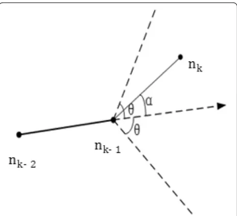
The random waypoint mobility model, RWP, used by the RSSI-MCL localization algorithm does not require high hardware requirements for nodes, but the mobile path is more random. As shown in Fig.1,nk−2andnk−1 respect-ively represent the location of the nodes in the two previous moments. Nodenk−1first selects thenknode randomly in the scene as the target location to be reached and move to the target with a random rateV∈[Vmin,Vmax]. Andα is the angle between velocity vk−1andvk.The motion of dif-ferent time periods is independent of each other, which may cause the randomness of nodes’ movement direction to be larger and impact locating performance. In Fig.1, the optimized model of motion, the position prediction equation of momentkis:
xik yik
¼ xik−1þvk cosð Þα Δkþnk
yik−1þvk sinð ÞαΔkþnk
ð15Þ
In the equation,Δkis the environmental impact factor andnkis the Gaussian noise.
2.3.3 The particle filter algorithm of importance weight optimization
Most of predicted particles’ weights are all very close to 0 after observation and weighted calculation. We need to do again for location updates and weighted calcula-tions to obtain a particle that has a certain number of weights approaching 1 after multiple iterations. To ac-celerate the gain of a particle approaching 1, in this paper, we adopt a particle filter algorithm based on im-portance weight optimization, introducing an influence factor to optimize the importance weight of the particle, and in the process of resampling, more particles will be duplicated to avoid particle dilution effectively.
In each resampling process, an influence factor α(0 <α< 1) is added to the weights after normalization, the weight of the particle changing into ðwi
kÞ
α
, and then normalized the weight, the value of particle i at moment k is:
~
wik¼ w
i k
α PN
i¼1 wik
α ð16Þ
The weight of each particle is retuned, and the weight of the small particles is improved after the optimization of weights, when contrary it gets reduced. The effective-ness of this method is proved by analysis as follows.
Fig. 1Majorizing particle motion model. Therefore, this paper optimized the movement direction of the RWP motion model and
limits the direction of the node’s motion to an achievable range,
which mean the angle between the next motion’s direction and the
original motion’s direction should less than the maximum angle that
can be achieved, as shown in the Fig. 1 thatθis the maximum
value ofα. Thus, to limitαtoθrange can avoid that the node in the
a
b
c
Suppose the particle set that is not normalized in time <wNk <1, and the weight after optimization is:
~
The small weight of particle will increase when its weight is optimized. And in the process of resampling the particle setfxi
t;wikg N
i¼1, more particles will be copied,
avoiding particle degradation effectively.
3 Comparison of MCL, RSSI-MCL, and RSSI-IMCL
3.1 Simulation environment
This paper’s simulation experiment uses MATLAB
platform, and the simulation experiment is set in a rectangular plane area of 200 m × 200 m. We assume that 40 beacon nodes are randomly distributed, the position is fixed, and the coordinates are known, and those 80 target nodes were moved randomly, in addition, their direction and speed is random as well, and the movement speed is not exceeding the preset limit. The maximum moving speed of the node is 50 m/s. Using the RWP model, the communication radius of the beacon node and the target node is both 50 m.
The positioning error used in this paper is defined as follows:
In equation, n is the number of locations,ris the ra-dius of communication, (xi,yi) is the actual coordinate of the target node, andðx0i;y0iÞis the coordinate information estimated by the algorithm.
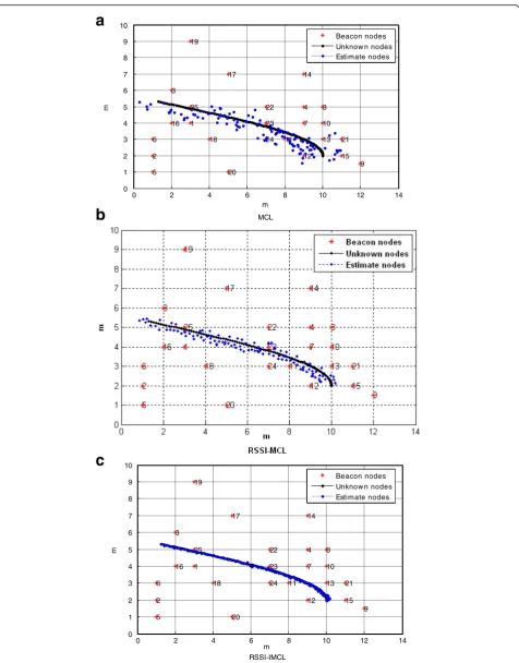
3.2 Comparison and analysis of network topology
What Fig. 2 shows is the topology diagram of MCL
localization algorithm, RSSI-MCL positioning algorithm, and RSSI-IMCL localization algorithm. As shown in Fig. 2a, the location of the estimated node is located around the target node. As shown in Fig. 2b, the esti-mated node location is near the target node, especially in the range of 6–10. As shown in Fig.2c, the location of nodes estimated by improved RSSI-MCL localization
0 20 40 60 80 100 120 140
the number of anchor nodes
th
algorithm is almost identical to the location of the target node, when compared to RSSI-MCL localization algo-rithm and MCL localization algoalgo-rithm, it shows better predictive effects.
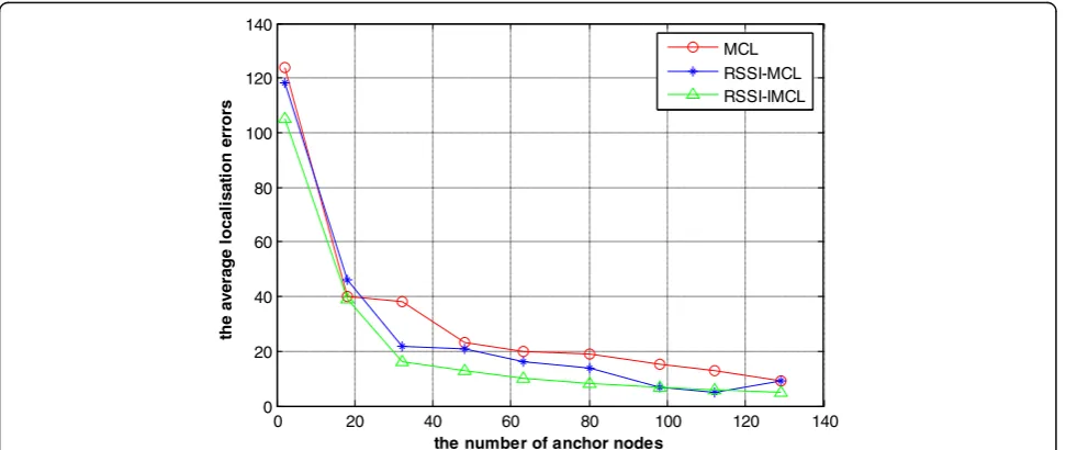
3.3 Comparison and analysis of anchor nodes’number
and localization errors
Figure 3 is the variation curve that the average
localization errors changed with the number of anchor nodes of MCL, RSSI-MCL, and RSSI-IMCL localization algorithms. With the increase of the number of anchor nodes, the average localization errors of the three algo-rithms are all decreasing. When the anchor node is within 20, the average localization errors of the three al-gorithms fluctuate greatly. When the number of anchors is close to 40, the average localization errors of the three
algorithms tend to be stable, and the error of the three algorithms is similar. But the RSSI-IMCL is slightly bet-ter than the other two algorithms.
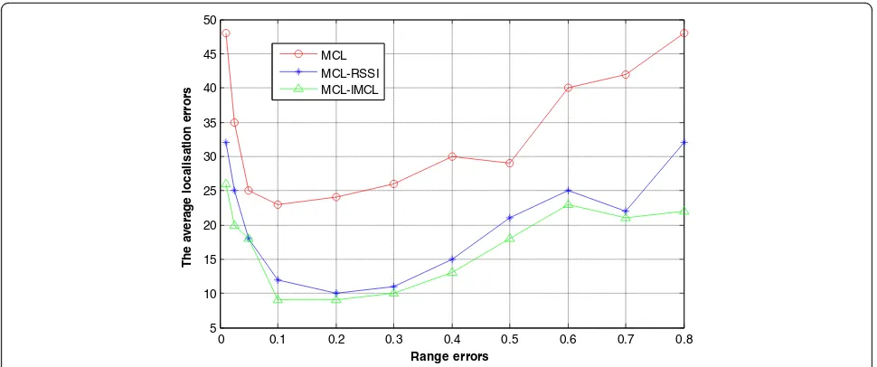
3.4 Comparison and analysis of localization errors and distance errors
What the Fig.4 shows is the curve that localization er-rors changed with the range error of MCL localization algorithm, RSSI-MCL and RSSI-IMCL. With the in-crease of ranging error, the average localization errors of the three algorithms are also increasing. However, it can be seen that RSSI-MCL is significantly better than the other two algorithms. When the range errors are be-tween 0.1 and 0.2, the average localization errors are minimal, then the positioning error gradually increased, so the range errors are optimal when between 0.1 and
10 20 30 40 50 60 70 80 90 100
15 16 17 18 19 20 21 22 23
The movement speed
T
h
e aver
a
g
e
l
o
cal
isat
io
n
er
ro
rs
MCL MCL-RSSI MCL-IMCL
Fig. 5Comparison of the average localization errors and the movement speed
0 0.1 0.2 0.3 0.4 0.5 0.6 0.7 0.8 5
10 15 20 25 30 35 40 45 50
Range errors
Th
e
a
v
e
ra
ge
l
oc
a
li
s
a
ti
on e
rrors
MCL MCL-RSSI MCL-IMCL
0.2. When the range errors going rewards 0.3, the aver-age localization errors began to rise.
3.5 Comparison and analysis of localization errors and movement speed
What Fig. 5 shows is the curve that the localization errors changed with the particle velocity of MCL, RSSI-MCL, and RSSI-IMCL. The average localization errors of MCL localization algorithm and RSSI-MCL localization algorithm has minimum when the velocity is 20, then with the movement speed increases, the error also increases. The main reason is that the node speed is increasing and the localization of the next node is in-creasing so that the non-conforming nodes are difficult to filter. The average localization error of RSSI-IMCL is relatively stable with the increase of velocity, which mainly because of historical trajectory prediction, optimization of particle weights, and the result of the updating particle set.
4 Conlusion
In this paper, the mobile node RSSI-IMCL algorithm in wireless sensor networks is proposed, and the random waypoint mobile model is improved. A Newtonian interpolation method is used to estimate the motion speed and direction of moving nodes at the current time. The degradation of particle subset was improved by op-timizing weight value. The experimental results show that RSSI-IMCL compares with MCL and RSSI-MCL in different ranging error, anchor node density, and motion speed. RSSI-IMCL algorithm improves network topology and reduces energy loss; the average positioning error was reduced and the positioning accuracy was improved. It is valuable to study the mobile node positioning tech-nology in Wireless Sensor Network. According to the ranging signal, when the distance error is greater, the lo-cation error of RSSI-IMCL algorithm will be greater, and how to accurately and quickly cover the network area is the next step. At the same time, the mobile path of the mobile sensor node will also affect the location perform-ance, so the mobile node location algorithm combined with routing and positioning is also the focus of future work.
Abbreviations
MCB:Monte Carlo Localization Boxed; MCL: Monte Carlo localization; RSSI: Received signal strength indication; RSSI-IMCL: Received signal strength indication improvement Monte Carlo localization; RWP: Random waypoint mobility model; SMCL: Sequential Monte Carlo Localization
Acknowledgements
The research presented in this paper was supported by Chao Hu University, Hefei, Anhui.
Funding
The authors acknowledge a key project from the Natural Science Foundation in Anhui Province, China (Grant: KJ2014A096).
Authors’contributions
JYL is the main writer of this paper. She proposed the main idea, proposed and deduced the RSSI-IMCL, completed the simulation, and analyzed the result. CW gave some important suggestions for the simulation. Both authors read and approved the final manuscript.
Competing interests
The authors declare that they have no competing interests.
Publisher’s Note
Springer Nature remains neutral with regard to jurisdictional claims in published maps and institutional affiliations.
Author details
1College of Information Engineering, Chao Hu University, Hefei, Anhui, China. 2
College of Information Engineering, Anhui Xinhua University, Hefei, Anhui, China.
Received: 19 March 2018 Accepted: 30 May 2018
References
1. Wang W, Zhu Q. Sequential Monte Carlo localization in mobile sensor networks[J]. Wirel. Netw, 2009, 15(4):481–495.
2. Chelouah L, Semchedine F, Bouallouche-Medjkoune L. A power adjusting anchors with improved localization algorithm for mobile wireless sensor networks[J]. Int. J. Comput. Math. Comput. Syst. Theory, 2017, 1(3–4):129–140. 3. Lei Z. Self-adaptive Monte Carlo localization for mobile robots using range
finders[J]. Robotica, 2012, 30(2):229–244.
4. Chelouah L, Semchedine F, Bouallouche-Medjkoune L. A power adjusting anchors with improved localization algorithm for mobile wireless sensor networks[J]. Int J. Comput. Math. Comput. Syst. Theory, 2017, 1(3–4):129–140. 5. Z Liang, X Ma, X Dai, Information-theoretic approaches based on sequential
Monte Carlo to collaborative distributed sensors for mobile robot localization. J. Intell. Robot. Syst.52, 157–174 (2008).https://doi.org/10.1007/ s10846-008-9206-9
6. Shen X, Yi Y, Dong W, et al. Mobile nodes localization based on adaptive particle swarm optimization and modified Monte Carlo localization boxed in wireless sensor networks[J]. Sens. Lett., 2014, 12(2):1–12.
7. A Alaybeyoglu, An efficient Monte Carlo-based localization algorithm for mobile wireless sensor networks. Arab. J. Sci. Eng.40, 1375–1384 (2015).
https://doi.org/10.1007/s13369-015-1614-0
8. Kadir H A, Arshad M R. Robust blimps formation using wireless sensor based on received signal strength indication (RSSI) localization method[J]. Sains Malaysiana, 2017, 46(1):129–137.
9. Álvarez Y, M de Cos, J Lorenzo, et al., Novel received signal strength-based indoor location system: development and testing. J Wireless Com Network
2010, 254345 (2010).https://doi.org/10.1155/2010/254345