Coalition Formation based Compressive Sensing in
Wireless Sensor Networks
Alireza Masoum1,†,‡,*ID, Nirvana Meratnia1,and Paul J.M. Havinga1,
1 Pervasive Systems, Department of Computer Science University of Twente, The Netherlands;
[email protected], [email protected], [email protected]
* Correspondence: [email protected]; Tel.: +31-68-251-0228 ‡ These authors contributed equally to this work.
Abstract:Compressive sensing originates in the field of signal processing and has recently become a topic of energy-efficient data gathering in wireless sensor networks. In this paper, we propose an energy efficient distributed compressive sensing solution for sensor networks. Proposed solution utilizes sparsity distribution of signals to group sensor nodes into several coalitions and then implements localized compressive sensing inside coalitions. This solution improves data-gathering
performance in terms of both data accuracy and energy consumption. The approach curbs
both data-transmission costs and number of measurements. Coalition-based data gathering cuts transmission cost, and the number of measurements is reduced by scheduling sensor nodes and adjusting their sampling frequency. Our simulation showed that our approach enhances network performance by minimizing energy cost and improving data accuracy.
Keywords:Compressive Sensing; Coalition; Sparsity; Belief Propagation; Joint Sparse Recovery
1. Introduction
Energy efficiency is a continuing concern within wireless sensor networks. Every sensor network is operational as long as they have enough energy resources. Therefore, to ensure the longevity of a network , energy efficient techniques are essential [1]. Compressive sensing is one of the new energy effecient compression based data gathering techniques which is introduced in recent years.
Compressive sensing is a concept originated from the field of signal processing. The promise of compressive sensing is that it can reconstruct sparse or compressible signals from a small number of measurements without having a priori knowledge about the signal structure. This technique utilizes information rate instead of sampling rate to sample and recover the signal [2].
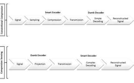
Unlike classic compression techniques, compressive sensing simplifies encoding procedures while making the decoding procedure more complicated. This characteristic is well suited for wireless sensor network data gathering applications. It employs simple encoding on the resource-restricted sensor nodes and a complex decoding procedure at the powerful base station. Figure 1illustrates the traditional data compression and compressive sensing techniques.
Recent compressive sensing solutions proposed in wireless sensor networks have proven advantages in minimizing the number of measurements, but they are still not competitive with the existing data compression techniques [3]. Since transmission cost is the dominant energy consumption parameter, compressive sensing methods should consider minimizing the consumption by each measurement in terms of transmission cost. In some proposed solutions, each sensor node produces its measurements, aggregates these with the measurements of other nodes and transfers them to the base station. Since sensor nodes may be far from each other, the transmission cost is high enough to negate the advantages of compressive sensing-based data gathering [4]. Utilizing distributed compressive sensing could represent an important step towards improving existing compressive sensing methods in terms of energy consumption, bandwidth use and data quality [5].
In this paper, we propose a new distributed compressive sensing based data gathering approach which utilizes spatial-temporal correlation to improve the network performance in terms of energy
Figure 1.Traditional data compression vs compressive sensing
consumption and data reconstruction accuracy. In the first step, we propose a spatial correlation based coalition formation algorithm to localize data collection of the sensor nodes. This approach leverages the sparsity distribution of signals in order to group spatially correlated sensor nodes into coalitions. Inside each colaition, we use the sparsity distribution of signals to define a utility function. This function later is used to minimize the number of active sensor nodes, which reduces energy consumption.
After coalition formation, a spatial temporal correlation based compressive sensing solution is proposed inside each coalitions. Proposed solution employs a block diagonal measurment matrix to produce a linear combination of sensor node readings. Block diagonal measurment matrix is structured in a way that balances the computation and communication load over the coalitions. This spatial-temporal correlation based compressive sensing is used inside each colation to compress sensor node readings and transfer it to the base station. Upon receiving compressed data, the base station applies a joint sparse signal recovery mechanism to reconstruct compressed data. In the first step, a joint sparse signal recovery is run to find the common sparsity profile among the coalitions. This recovery procedure then executes inside each coalition to achieve a common profile among sensor nodes. Utilizing this recovery algorithm helps to achieve better accuracy in data reconstruction while the number of required measurements is reduced.
On the other hand this paper analyses the impact of different transform basis on compressive sensing. The compressible or sparse signal may be represented in different transform bases. Choosing the appropriate transform basis is essential in sparse representation, which can lead to less measurements and more accurate signal reconstruction during the recovery phase. To the best of our knowledge, the selection of an appropriate transform basis has not been adequately studied, as most existing compressive sensing techniques have focussed on optimizing reconstruction algorithms. This paper classifies different signals based on their characteristics and investigates the assignment of an appropriate transform basis for each specific type of signal.
coalitions, respectively. Data reconstruction procedure is mentioned in Section7while Section8
analyzes the performance of the proposed scheme. Finally, conclusions are drawn in Section9.
2. Related Works
The study presented in [14] introduces a belief-propagation-based compressive sensing technique that considers the temporal correlation model of the signal as given information and employs it to reconstruct the signal. To model temporal correlation, one can decrease the number of required measurements and help to achieve better reconstruction accuracy with a specific spike-and-slab Markov model. The accuracy of this Markov model changes over time, and this can influence reconstruction accuracy. Therefore, this algorithm periodically analyzes the model parameters and employs an online estimator to predict its parameter. This estimator is based on sequential expectation maximization (EM) algorithm that is derived by maximizing the Kullback-Leibler (KL) information measure. At the end of each reconstruction period, this estimator refers to reconstructed signal coefficients for the last time period to update the Markov model parameters. This approach focusses on robust accurate data reconstruction and decreases the number of measurements. However, the energy efficiency of this solution is not addressed explicitly.
The authors of [18] discuss how to make the encoding process more efficient in terms of resource management strategy. They proposed a compressive sensing approach that considers temporal correlation among sensor node readings to recover the original signal. They combined their compressive sensing approach with gossip-based routing to recover the sparse signal in multi-hop wireless sensor networks.
In the case of telemonitoring applications, most signals, like ECG signals, are not sparse in the time domain. Therefore, current compressive sensing solutions cannot provide accurate reconstruction. To address this problem, one study [19] addresses a block-sparse Bayesian learning-based compression technique. The proposed solution represents an extreme performance improvement in recovering non-sparse signals. Furthermore, using the block structure to recover signals lessens reconstruction complexity, which results in lower computational cost and better accuracy.
A combination of model-based data prediction and compressive sensing is addressed in [20] to achieve energy-efficient data gathering in sensor networks. Compressive sensing facilitates the compression of sensor node readings while an adaptive data prediction model is built on this basis, reducing the data sampling frequency. Using this data prediction model, sensor nodes do not require any prior information regarding monitored signals and can adapt their sampling rates to the time-varying sparsity level of the signals. Minimizing the data-sampling rate based on the sparsity level of the signal provided by compressive sensing attenuates the data-transmission rate, which conserves power.
Luo et al. [21] present a compressive data-gathering (CDG) method, which combines data compression and routing for data collection in large-scale wireless sensor networks. The result of this combination is a balanced distribution of energy drain over the network, which improves network lifetime. Furthermore, it shows a significant reduction in communication cost. With regard to scalability, this solution cannot be applied in small-scale networks and large-scale dynamic networks.
A further study [22] introduces a joint sparse signal recovery method which assumes sensor nodes have been distributed into different clusters, and uses a joint sparse signal recovery mechanism (instead of an independent reconstruction process) to recover the compressed data. This solution solution minimizes energy expense in terms of data compression and transmission rates. However, it does not ensure that application-defined data accuracy requirements are met.
[24]. It takes advantage of spatial correlation among sensor node measurements and aims primarily to achieve good recovery accuracy. Furthermore, it concentrates on reducing the number of data transmission and reception parameters, which results in energy-efficient data gathering. To do so, the proposed solution adjusts the probability of forwarding received data packets to the number of neighbor nodes. This approach ignores the noise and error parameters in the transmission scenario.
The research presented in [25] is one of the first studies to propose a compressive sensing-based data-gathering solution based on a random walk algorithm. The authors employ this algorithm to produce a non-uniform random measurement matrix. To do so, randomly selected sensor nodes in each walk generate a measurement based on linear combination of both the node itself and neighboring nodes’ observations. At the end of each random walk, the measurements produced are forwarded to the base station. Compared to the existing random projection solutions, this approach shows a significant reduction in data-transmission cost.
A compressive sensing-based false data detection and correlation framework for crowd sourcing applications is presented in [26]. In crowd sourcing applications, a large number of participants employ their mobile devices to collect environmental data and report it to the base station. Misbehaving or erroneous participants can produce faulty data and packet loss in the network. Missing or faulty data is reconstructed with a spatial-temporal correlation-based compressive sensing technique. This approach considers collected data as multidimensional time-series and groups sensor nodes into smaller grids based on their location. In the first step, this solution gathers raw data from participants as a training data set and groups them into different grids by considering spatial correlation among sensor nodes. Then, the compressive sensing algorithm reconstructs the sensor data with spatial-temporal correlation and the low-rank feature among sensor node readings. The proposed solution guarantees high data quality in environments with high packet loss and noisy characteristics, but the study did not address energy savings.
A hybrid network coding and compressive sensing-based solution in [8] represents a clustered spatial-temporal correlation-based compressive sensing method. Each sensor node applies a well-defined Gaussian code matrix to encode its reading and forwards it to the base station. Proper selection of the measurement matrix and network coding coefficients is utilized at the base station to implement a low-complexity data reconstruction algorithm that reconstructs data more accurately. In addition, the proposed solution reduces the number of measurements, resulting in energy-efficient data transmission.
The authors of [9] proposes a novel compressive sensing-based data-gathering solution for massive lossy data-transmission scenarios. The proposed compressive sensing solution models environmental data dynamicity using an environmental matrix (EM) and then employs the spatial-temporal correlation observed in this matrix to reconstruct the data. Furthermore, this approach has a multiple attribute assistant (MAA) component, which correlates environmental attributes to discover data loss patterns in reported encoded data. Combining MAA and EM, the compressive sensing-based reconstruction method provides better reconstruction accuracy. However, this approach suffers from higher computational complexity.
size. In addition, the dynamic adjusting window size modifies the number of required measurements, which results in adaptive data transmission.
3. Preliminarities
3.1. Compressive Sensing
This section presents the mathematical description of compressive sensing theory as presented in [27,28].
Let us assume that a discrete signal denoted byX∈RNrepresented byN×1 column vector has sparse representation in some basis (for example in fourier or wavelet basis). Considering the sparsity concept, this signal can be expressed in terms of its basis as follows:
X=ΣNk=1akψk =Ψa (1)
, where Ψ is an N×N orthogonal basis matrixΨ = [ψ1,ψ2, ...,ψN], ψi , i = 1, 2, ...,N and a= [a1,a2, ...,aN]is anN×1 column vector of the coefficient sequence ofXinΨdomain.
SignalXis compressible or sparse inΨbasis if most of the elements inaare zero. Compressive sensing theory states that if signal X is K-sparse on Ψ basis, it can capture and recover from M
non-adaptive, linear measurements(K<M<<N)with a certain restriction.
Compressive sensing theory also states that, rather than acquiring the entire signal and then doing compression, it should be possible to construct a sampling framework to capture only the useful information in the sparse signal to begin with. The sampled signal via compressive sensing is described as follows:
Y=ΦX (2)
, whereY = [y1,y2, ...,yM]is theM×1 measurement matrix,Φ = [φ1,φ2, ...,φM]represents a M×Nand eachφi,i=1, 2, ...,NisN×1 vector. It should be noted thatΦis a random matrix, which
can be considered a second basis. Each elementaryyiin the measurement matrix is a product ofXand vectorφifrom the sensing matrix. We can replaceXwithΨaand rewriteYas:
Y=ΦX=ΦΨa=Θa (3)
,whereΘ=ΦΨis aM×Nmatrix.
Compressive sensing demonstrates that sparse signals can be recovered fromMmeasurements if the process can satisfy the restricted isometric property (RIP) [29,30]. The RIP states that the correlation betweenΦandΨmust be low (be incoherent) to restrict the number of measurements required to recover the signal. Coherence is a metric to measure the maximum correlation between any row ofΦ and any column ofΨand can be defined byµthe as follows:
µ(Φ,Ψ) =max1≤k,j≤N|<φk,ψj>| (4)
When comparingΦandΨ, if the relationship between them is weak, the condition is called incoherence. Formally speaking, matrixΘof sizeM×Nsatisfies the RIP of orderKif it is a minimum number such that
(1−δk)kak22≤ kΘak22≤(1+δk)kak22 (5) , whereδk∈(0, 1)is a restricted isometric constant (RIC). Equation3must hold true for all values
The RIP guarantees the exact recovery ofXwith a high probability if
M≥CKlogN
K (7)
, whereNis the dimensionality of the original signal andCis the small positive constant. This formula is a conservative estimate of the lower bound on the number of measurements required to recover the original sparse signal. SinceKrepresents the amount of important information inside the signal, we can conclude that the number of required samples to recover the signal is proportional to the information content of the signal.
The recovery of the signalXfromYis an NPhard problem, but it can be achieved through optimization. To do so we can usel0minimization as follows:
´
a=arg min
a∈RNkakl0 s.t. Y=ΦX. (8) , where ´X = Ψa´, ´X is the recovered signal and ´ais the optimal estimation for a. Since l0 minimization is computationally intractable,l1minimization is widely used for compressive sensing signal reconstruction. We can recover the coefficients of sparse signalaby solvingl1norm minimization as follows:
´
a=arg min
a∈RNkakl1 s.t. Y=ΦX. (9)
3.2. Distributed compressive sensing
Standard compressive sensing methods can be implemented on single sensor node. However, sensor networks consist of many sensor nodes distributed over the network. These sensor nodes have spatial and temporal correlation among their readings. Given this distribution, distributed compressive sensing is proposed as a standard compressive sensing method for several sensor nodes [?]. In this distribution, each sensor node employs compressive sensing theory to encode its reading and transfer it to the base station. For the reconstruction procedure, the base station utilizes joint sparse signal recovery to recover all encoded signals precisely.
Joint sparse signal (JSM) recovery involves a set of signals that are jointly sparse. Each joint sparse signal can be represented by a combination of the common part and the innovative part [33]. There are three different joint sparsity models that can be used to recover the original signals. In this case we have an ensemble of signals with notation and measurement models as follows:
Each signal is denoted byxj,j∈ {1, 2, ...,J}wherexj ∈ RN. For this model, it is assumed that
there is a known sparse basisΨforRNin which eachxjcan be sparsely represented. On the other hand, each signalxjis assigned a measurement matrixΦwhich isMj×N. Based on this definition, a
measurement signal for each signaljcan be represented byyj =φj×xj.
In what follows, we introduce three different types of joint sparse models.
3.2.1. Joint Sparse Model Type-1
The joint sparse model type-1, called JSM1, states that all signals reported by sensor nodes have a common sparse component while each individual signal contains an innovative sparse component.
xj=zc+zj with zc=Ψac, kak0=K and zj=Ψaj, kajk0=Kj. (10)
where thezcis common to the all of values forxjand its sparsity level is the minimum sparsity level of all the signals in base functionΨ. Signalzj is the specific innovative part ofxjand has its
of the common part to increase the reconstruction accuracy. When the proportion of the common part is far more than individual part, the reconstruction error decreases.
3.2.2. Joint Sparse Model Type-2
The Joint sparse model type-2, namely JSM2, assumes that signals have the same sparsity set profile, however, their coefficients are different. In this model we formulate each signal as:
Xj =Ψaj (11)
, whereajis non-zero in the common coefficient profile. This models data for the sensor nodes
that are deployed in the environment and observe the same signal, but due to signal propagation effects, receive the signals with a phase shift.
3.2.3. Joint Sparse Model Type-3
There is some similarity between Joint sparse model type-3 (JSM3) and JSM1, but the common profile is no longer sparse. As with JSM1, we formulate the signal as follows:
xj=zc+zj with zc=Ψac, kak0=K and zj=Ψaj, kajk0=Kj. (12) In this representationZcis not sparse. This model is applicable for environments in which several signals are produced from different sources with a background signal that is not sparse.
3.3. Sparse transform basis
Compressive sensing must utilize an appropriate transform basis to provide an accurate sparse representation for a compressible signal. The selection of these transform bases is very important and relates to the nature of the data or the signal to be compressed. In this section, we propose a classification for signals and then introduce an appropriate transform basis for each of them.
3.3.1. Classification
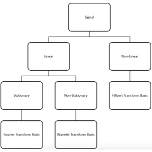
A signal is a physical quantity that is measurable. Various classifications of signals have been suggested based on the nature of the signal and the system that produces it. These include continuous versus discrete, periodic versus non-periodic, energy versus power, deterministic versus random, stationary versus non-stationary, and linear versus non-linear [34,35]. In our study, we classify existing signals into a linear and non-linear signals. Linear here means that the natural frequencies of the signal are not dependent on the amplitude of oscillation. A signal can also be stationary or non-stationary. A stationary signal is one whose frequency or spectral contents change over time.
Figure 2.Signal classification and appropriate transform allocation
Based on the proposed signal classification, in this section we introduce wavelet, fourier and hilbert transformations and discuss which transform basis belongs to which type of signals.
The fourier transform is suitable for a wide range of purposes, such as signal transmission and stationary signal processing. However, this transform is not appropriate for non-stationary signals because it cannot provide any information about signal frequency changes as a function of time for these signals. To cope with this limitation, the short time fourier transform (STFT) employs a fixed-size window to segment the signal into stationary parts but suffers from time or frequency resolution depending on its window size [34]. Most of the compressive sensing-based data-gathering approaches in wireless sensor networks use the FFT as their basis [46,47]. This basis implements transformation over the entire length of the signal. In signal reconstruction, this transform basis provides no information about time resolution and as such fails to report damage locations since all possible time information is lost. The STFT makes location information available. Although it provides a time-frequency representation of a signal, there is a major drawback with respect to utilizing STFT due to the fixed size of its window width [46,48].
The Wavelet Transform (WT) is a time-frequency technique that overcomes the poor time/frequency resolution and fixed-size window limitations of the STFT. In contrast to the FT, the WT is well localized, and with it few coefficients are needed to represent local transient structures. Therefore, the wavelet basis provides sparse representation of piecewise regular signals, which may include transients and singularities [35,49].
The WT can be either continuous or discrete. The Discrete Wavelet Transform (DWT) is used for signal decomposition, while a Continuous Wavelet Transform (CWT) is used for spectral analysis [50]. Decomposing the CWT produces wavelet series. These series are highly redundant and their computation is costly and time-consuming. The DWT is a fast computation of WT which reduces time and resource cost [50]. Wavelet Multi Resolution (WMR) is a method that implements DWT with filters. It employs a high-pass filter to process rapidly changing details (high-frequency components) and a low-pass filter to find slowly changing features (low-frequency components). In contrast with the WMR, the Wavelet Packet Transform (WPT) is a method that decomposes both wavelet details and wavelet approximation components at each level. Wavelet packets inherit properties such as orthonormality and time-frequency localization from their corresponding wavelet functions [35,49].
There are number of basis functions that can be utilized as a mother wavelet for the wavelet transform, including Haar wavelet transform, Symlet wavelet transform, Coiflet wavelet transform, and Meyer wavelet transform. In terms of the signal characteristics and the attributes of specific wavelet transforms, each of them can be employed to represent sparsity of signal. The WT’s ability to provide good frequency resolution for high-frequency signals and time resolution for low-frequency signals makes this technique a good basis for non-stationary signals that require time and frequency resolution [35,50].
Hilbert transform is another transform basis which takes a function as an input and produces a function with the same domain. The Hilbert transform can be either continuous or discrete. The non-linearity and non-stationary nature of some signals make the Hilbert transform a powerful tool as the transform basis for signals with those properties. Hilbert transform decomposes a signal posteriori, enabling the extraction of the inner scales of each signal [35].
3.4. Belief Propagation
C1
C2
C3
. . .
Cm
X
Cm-1
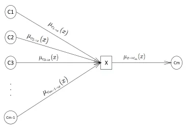
Figure 3.Message from variable node to the connection node
1. Edges or messages from a variable node to the connection node:
These edges contain probability which is calculated by gathering all incoming edges (excepts edges coming from nodecm) and multiplying them, which is described as follows:
µx−→c(x) =
∏
x∈N(x)\{c}µv−→x(x) (13)
, whereµv−→xshows the edges from nodevto nodex,N(x)denotes the neighbor nodes ofx
andN(x)\{C}denotes the neighbor nodes ofxexcept for nodeC. For an example, see Figure3, which shows part of a factor graph. The message from variable nodesXto the connection node
cmis given by:
. . .
Xm-1
X3
X2
X1
Xm
C
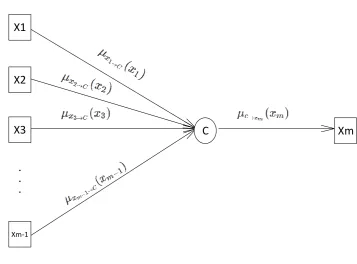
Figure 4.Message from connection node to variable node
2. Edges from a connection node to the variable node:
This probability is computed by obtaining all the incoming edges to nodeCexcept the link from nodex, multiplying them byCand finally finding the sum of all connected variable nodes except for nodex. In general, the edges going from the connection nodes to the variable node can be described as follows:
µc−→x(x) =
∑
∼{x}
c(N(c))
∏
v∈N(c)\{x}
µv−→c(v) (15)
, whereN(C)is all variable nodes connected toCandσis the sum of all connected variables except forx. µv−→c(v)shows the edges from variable nodev to the connection nodeC. An
example is seen in Figure4, which shows part of a factor graph. The message from connection nodesCto variable nodexmis represented by
µc−→xm(xm) =
∑
(x1,x2,...,xm−1)
c(x1,x2,...,xm−1)×µx1−→c(x1)×µx2−→c(x2)×
...×µxm−→c(xm)
(16)
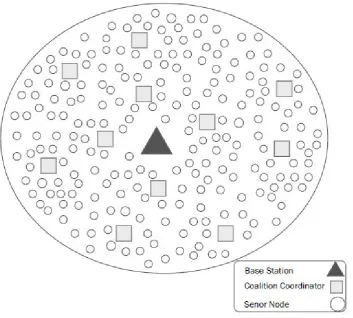
3.5. Network Model and Assumptions
Figure 5.Network architecture
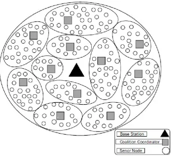
Figure 6.Coalition representation
The sensor nodes are grouped into coalitions. To form these coalitions, we consider the sparsity distribution of signals among sensor nodes and place all correlated sensor nodes in the same group (Figure6).
4. Overview of the Proposed Approach
In order to achieve an energy-efficient and quality-aware compressive sensing method, we introduce a distributed compressive sensing approach with spatial correlation among sensor nodes to group them into coalitions. The proposed coalition-formation method is represented by a block diagonal measurement matrix in which each diagonal entity corresponds to one of the coalitions. Upon forming coalitions, the proposed spatial-temporal correlation-based compressive sensing approach is implemented inside each coalition in order to schedule sensor nodes and encode their readings. Temporal correlation among sensor node readings allows our approach to adjust the number of measurements with regard to the temporally changing sparsity level.
After applying propsed compressive sensing solution inside each coalition and forwarding compressed data, the base station employs a two-step joint sparsity-based recovery algorithm to reconstruct the original signal. In the first step, it runs joint sparsity model to find the common sparsity profile among the coalitions. In the second step, it calculates the common sparsity model within each coalition, which allows it to achieve data reconstruction with high accuracy and fewer measurements.
We summarize our contributions in this paper as follows:
each coalition according to the temporal sparsity level of the signal.
• Proposing a two-level belief propagation-based reconstruction algorithm that provides acceptable data quality in terms of data accuracy.
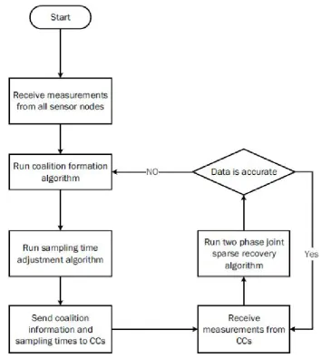
For a graphical view of the entire data-gathering procedure proposed in this paper, see the flowchart in Figure7. This flowchart will be described in more detail in the following sections.
Figure 7.Approach overview flowchart
5. Coalition Formation
coalition we remove the redundancy among compressed measurements of different sensors, decreasing the number of data packets.
The compressive sensing-based coalition formation introduced here is inspired by the fact that the subject signals are distributed in the environment. On the other hand, the distribution of the signal elements is different for the sensor nodes based on their locations. Therefore, the sensor nodes observe the same signal with different resolution. On the other hand, the sparse representation of the signal can be shown in a sparsity base function. We apply the base function distribution over the network to define a cover parameter. This cover metric shows the degree of the base function covered by the sensor nodes. This parameter helps sensor nodes inside each coalition produce informative measurements, which results in accurate data recovery by the base station.
To make a concrete and accurate coalition, we define a utility function U based on cover, transmission and sensor node correlations. This function is used to evaluate the efficiency of the coalitions produced. To do so,Umakes a trade-off between reconstruction accuracy (correlation between sensor nodes and base function distribution pattern) and data-transmission cost (distance between sensor nodes).
The following sections explain the prerequisites for the coalition-formation algorithm and conclude by presenting its procedure.
5.1. Measurement Matrix
Since we divide the network into different coalitions, the data is gathered through these different coalitions. Therefore, whole data may be divided into discrete blocks, in which each block is acquired via a local measurement operator. Assuming that we have divided the network intoNCcoalitions and our signalXis partitioned intoNCblocksX1,X2, ...,XNC ∈R
N. Each blockjwhich shows coalitionj
is assigned with a local measurement sub-matrixΦj :RN→RNj. Each measurement sub-matrixΦj represents the measurement pattern in each coalitionj.
Each of our measurement sub-matrixesΦjis assigned to one coalition matrixC, which permutates the entities of the original signal assigned for the specific coalition j. In order to assign each coalitionj, through its measurement matrixΦjwith the permutated signal coefficientsxC
j, we multiplyCwithX
which producesCX=XC= [x1C,xC2, ...,xCNC]and finally we have:
Y=ΦCX (17)
, where: Φ= Φ1
Φ2
0
.
0
.ΦNC
(18)
The resulting matrixΦCrepresents the distribution of sensor nodes inside each coalition andCis a coalition matrix.
Based on Equation18and sparse representation of the signalX=Ψeawe obtain:
Y=ΦCX=Φ(CΨe)a=ΦΨa (19)
, whereΨ=CΨe is a permutated version ofΨe. As we have seen, our coalition matrix permutates the base functions. Through this permutation, each row inΨis a permutated row ofΨe as follows:
ψiT=
N
∑
j=1
After permutation with the coalition matrix, we have a proper pattern for eachΦ to measure data from the sensor node inside each coalitionj.
The coalition-formation mechanism proposed here leads to a block diagonal measurement matrix with the appropriate coalition matrixCrelative to the location of the sensor nodes.
5.2. Utility Function
The proposed coalition matrixCcan be assigned to any coalition-formation method. During the coalition-formation procedure, we aim to make the best trade-off between energy savings and reconstruction accuracy. To do so, we introduce a utility function to evaluate the efficiency of the coalition-formation process. This utility function is defined based on the energy, correlation and cover degree parameters. The following sections explain these parameters in more detail and conclude by introducing the utility function.
5.2.1. Energy
We define the energy parameter for coalition-formation scenarios based on transmission, processing and measurement costs. Energy consumption is described as follows:
Ei=Ecomm+Epro+Emeas (21)
, whereEcomm,Epro,Emeasare communication, processing and measurement energy parameters, respectively. In this section, we focus on data transmission and measurement cost. We normalize these costs and replace energy requirements for the processing and measurement with the measurement costs. The transmission cost relates directly to the distance, while the measurement cost is influenced by the number of measurements. We replace the energy parameter with the normalized parameters of distance between two nodes inside the coalition and the number of measurements is represented as follows:
ECo(i,j) = Dist(i,j)
Distmax + Mi
Mmax (22)
, whereECoiis the energy cost in terms of the normalized distance between nodesi,j Dist(i,j) and the normalized number of measurements taken by nodei(Mi).
5.2.2. Correlation Degree
Since sensor nodes are located close to each other and they sense the same signal with different resolutions, we are able to find different levels of spatial correlation among them. Existing compressive techniques usually ignore this correlation and transfer redundant compressed data, which costs energy. Our approach tries to remove the redundancy among compressed data, thus leveraging this spatial correlation. To do so, in the coalition-formation phase we force the algorithm to consider this correlation along with other parameters. When we have correlated sensors in the same coalitions, we remove redundancy in the compressed data using the algorithm described in the next section. The correlation metric among sensor nodes is defined asCorr.
Corr(i,j) = Cov(yi,yj) σ(yi)σ(yj)
(23)
According to this formula, we define a binary variableCRwhich indicates whether two sensor nodes are sufficiently correlated. For this purpose, we rely on a user-defined correlation threshold
CR(i,j) = (
1 i f Corr(i,j)>TH1; 0 i f Corr(i,j)≤TH1. 5.2.3. Cover degree
Measured signals can be represented by a sparsity function distribution over the networks. These functions can also be grouped into one or more coalitions. The performance of our coalition mechanism in terms of recovered data accuracy greatly depends on the nature of the sparsity base functions. To evaluate this performance, we define a sparsity base cover degree ((SCD)) metric, which measures the degree of overlap between each coalition with base functionsΨ. Essentially, theSCDshows the energy overlap between the base functions and coalitions.
We define theSCDmetric between each base functioniand coalitionColjas follows: SCD(j,i) =
∑
m∈Colj
ψ2(i,m) (24)
, wheremis a sensor node located in coalitionj. This metricSCD(j,i)indicates that measurements collected from coalitionjcontain information about the measurements of other coalitions that cover the same base functioni. Taking this coverage degree among different coalitions into account, we use a joint sparse signal recovery approach to recover the original signal. However, there are situations in whichΨis covered only by one coalition. This means that for a K-sparse signal, the sparsity bases are contained in one coalition. Since this coalition is not known beforehand, we need to gather data from all coalitions, which is not energy efficient. Meanwhile, for accurate data recovery we must have
O(KlogN)measurements, meaning that we needO(KNClogN) measurements from all coalitions. On the other hand, the redundant measurements from other coalitions that do not overlap with the base, do not contribute to improving data accuracy. IfΨhas even overlap among different coalitions, our data recovery accuracy is increased. To quantify the cover level ofΨover coalitions, we define the maximumSCDas follows:
SCDmax(Ψ) =SCDmax(CΨ) =maxj,u
∑
wΨj2
(w,u), SCD(Ψ)∈[0, 1] (25)
SCDmaxshows the maximum cover level of each coalition with the sparsity base, whileΨjis the base sub-matrix assigned to coalitionj.
Forming coalitions such that the sparsity function can be recovered with several coalitions increases the quality of the recovered data. On the other hand, we must lower the number of correlated coalitions and the number of measurements to cut energy consumption. To find this balance, we must define a utility function as described in the next section. We discuss the number of coalitions and measurements and howSCDmax makes a trade-off between energy and quality in terms of the minimum number of measurements and data recovery accuracy.
5.2.4. Utility Function Formulation
In this section, we calculate a utility functionUto evaluate the candidate coalition structures. In the coalition-formation phase, we aim to buildNCcoalitions to achieve minimum energy
consumption while meeting data-quality requirements. Minimizing transmission and measurement costs, which is the main energy consumption parameter here, depends onSCDmax,MiandDistij.
The proposed utility function should evaluate adding a new sensor node to any coalition in terms of the trade-off between energy and quality. To do so, we define the utility functionUfor each combination of(ni,Colr)as follows:
5.3. Coalition Formation Algorithm
In the model introduced in this paper, the network consists of N sensor nodes SN =
{n1,n2, ...,nN}and L = {lni,nj}is the set of all possible connections between sensor nodes. Two sensor nodes are considered to be connected if they are placed in communication range of each other. We assume thatΨis known and all sparsity bases are normalized to 1 so thatSCD ∈ [0, 1]. This algorithm aims to cut energy consumption, provided that the data-quality requirement is met. Adding a new sensor node to the coalition is a selection procedure that evaluates which coalition is the best candidate for adding a sensor node. To make a good selection we run an optimization algorithm onU.
Before describing the optimization algorithm, theSCDparameter must be redefined. During coalition formation, when we add a new sensor node to the coalition,SCDevaluates the effect of adding this node by assigning a weight for the link between existing node in the coalition and the new sensor node. Our coalition-formation method, in order to examine the effect of adding a sensor node to each coalition, defines theSCDfactor asSCDmax(lni,nj,Colr)by considering the link,lni,nj ∈ L and a given coalitionColr. This link does not connect two nodes in the same coalition, which means
ni∈Colr and nj 3Cr.
Now we redefine the utility functionUfor each combination of(lni,nj,Colr):
U(ni,Colr) =CR(ni,nj)×(ECo(lni,nj) +αSCDmax(lni,nj,Colr)), α>0 (27)
SCDmax(lni,nj,Colr) here represents the maximum cover level when a new node is added to coalitionColrusing the linklni,nj.
Now we can formalize our optimization algorithm. The main goal in the improvement procedure is to lessen energy consumption and data recovery errors by adding new sensor nodes to the coalitions. When selecting an appropriate coalition for a new sensor node, the optimization algorithm examines the utility of adding the new sensor node to each coalition. For each coalition, this utility is defined based on the link connecting the new sensor node to an existing node in the coalition. Running the optimization algorithm finds the coalitions that pare down utility function’s link cost. We formulate this optimization as follows:
(ni,lmin,Colrmin) =arg minU(ni,Colr) =arg min[CR(ni,nj)× (ECo(lni,nj) +αSCDmax(lni,nj,Colr))] subject to ni ∈SN, nj∈Colr, CR(ni,nj)∈ {0, 1}
(28)
Now let us describe the algorithm according to the optimization equations. To find a set of sensor nodes for each coalition, this algorithm uses Equation28to find a set of links such that the totalUof the links is minimized. In the initialization step, we assume a set of candidate nodes and candidate links to be added to the coalitions defined by a set ofSNandL. The algorithm then assigns each coalition coordinator nodeCCto one of theNCcoalitions. In addition, it definesSNColrandLColr as a set of sensor nodes and connections of coalitionr, respectively. Along with the initialization step, the algorithm runs an iterative procedure where in each iteration, it allocates one sensor node to one of the coalitions. To do so, it first finds the utility function for all possible connections defined inL. It then runs the optimization function defined in Equation28and finds the minimum utility. However, it finds the utility for sensor nodes which satisfy the minimum correlation requirements. The output of this optimization is a connection link with minimum utilitylmin. This link connecting(ni,nj), adds
nodes. This procedure continues until all sensor nodes are assigned to the coalitions. Algorithm1
represents this coalition formation procedure.
Algorithm 1Coalition formation
1: SN=n1,n2, ..,nN
2: DefineL=lijas a set of all possible links
3: DefineNCcoalitions with one coalition coordinator 4: Define set of nodesNcolk and links for each coalitionsLcolk 5: for(P=1;P≤(N−NC);P+ +)do
6: for(Q=1;Q≤ |L|;Q+ +) do 7: Find Lposs=lij; i∈Ncolk,j∈SN 8: end for
9: CacluateU(Iij,Colk) 10: AddnjtoColkmin 11: AddlmintoLColmin 12: Find(nj,lmin,Colkmin)
13: RemovenjfromSN
14: RemovelminfromL 15: end for
6. Data Gathering Inside Coalitions
For the sensor nodes inside each coalition, we use a distributed compressive sensing technique to take measurements and recover the original signal. Before describing the data-gathering approach, in this section we take advantage of theSCDparameter to find the minimum number of active sensor nodes inside each coalition. The active sensor nodes inside coalition send their reading through a multi-hop network structure to the coalition coordinator.
6.1. Number of Active Sensor Nodes
In this section, we identify the number of sensor nodes required to be active for each coalition. This requirement helps to implement scheduling among sensor nodes and put some of the sensor nodes into sleep mode. Since the number of active sensor nodes measuring the signal is in direct relation with the number of measurements, we use Equations4and7to find the number of active sensor nodes.
To do so, we first define a minimum threshold based on Equation4to measure the minimum data reconstruction quality. We then measure the probability of having coherence, as defined in Equation
4, higher than this threshold to make sure that the number of sensor nodes is enough to recover compressed signal with high accuracy. This probability is defined and represented as follows:
If all measurement matrixesφjare orthogonal and the sparsifying basis functionΨe and coalition-formation matrix C are known a priori, thenµ(θ)is bounded as follows:
Pr[µ(θ)≤O r
SCDmaxNC
N logN)] =1−O(
1
N) (29)
Considering Equation29and Equation7, we can define the maximum number of sensor nodes required for providing high quality data as follows:
NANodes=O(SCDmaxKNClog2N) (30)
Fine-tuning the coalition-formation matrix leads to a smallerSCDmax, which in turn produces a lower number of sensor nodes while still ensuring data quality. The number of active sensor nodes associated with each coalition is dependent on itsSCDmaxlevel. Coalitions, which cover more sparsity functions, are more informative. Therefore, we must gather more data from those coalitions.
6.2. Compressive Sensing based Data Gathering
We now construct a block diagonal measurement matrix using the spatial-temporal correlation among sensor nodes.
LetSNColj = {1, 2, ...,Nj}denote the set of sensor nodes for the jthcoalition wherePjof these sensor nodes are randomly scheduled to be active. In contrast to existing compressive sensing methods, we define a new structure for the measurement matrix that is compatible with our coalition-formation method. We use a temporal block diagonal measurement matrix,Φt, to gather data. During each
sampling instance, we gather spatial observations of all sensor nodes at timetand produce a discrete spatial signal Xt at this time. The temporal observation of all active sensor nodes together is a spatial-temporal signal[Xtr1,X2tr, ...,XtrST], whereSTis a parameter representing the number of samples in each sampling round T. Each sampling period consists ofT sampling instances equal to the Shannon-Nyquist rate. To reduce this number of sampling times, the base station adjusts the number of sampling times according to the signal sparsity level and defines a number of sampling pointsST
for each sampling period.
For each sampling periodt, we considerΦtas a measurement matrix;Φtis aPj×SNColjmatrix. The measurement vectorYColj consists ofSTj sub-vector ofST sampling times such that Y
Colj =
[Y1tr,Y2tr, ...,YSTtr
j]where eachYiis aPj×1 vector.
Inside each coalition, we utilize a block diagram measurement matrix that compactly represents several temporal measurement sub-matrices. Combining these spatial-temporal measurements together yields:
Yj=YColj =ΦjXj (32)
YJ = Y1 Y2 . . . YSTj = Φ1
Φ2
0
.
0
.ΦSTj X1 X2 . . . XSTj (33)
, where for each 1≤t≤ST,ΦthasPjrows andSNColj columns. At the end of each sampling round, every sensor node transfers its measurement vectorYjto its neighbor node. The neighbor node
receives the data and forwards it to the coalition coordinator.
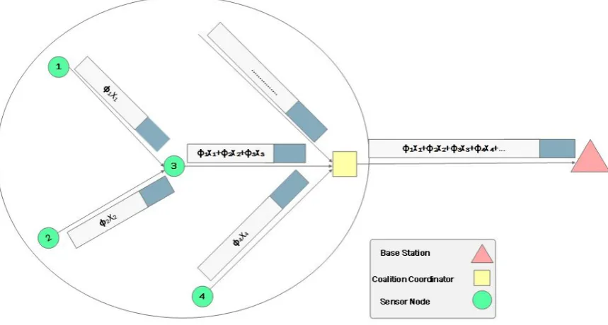
Introducing this temporal block diagonal measurement inside each coalition provides energy-balanced data aggregation within the coalitions. For instance, consider the sample coalition in Figure 8, where active sensor nodes forward their compressed data through active neighbor nodes to the coalition coordinator. Existing compressive sensing-based data collection approaches introduce unbalanced data transmission, which leads to communication and data overhead in the network. In our approach, each sensor node transfers a total ofMnumber of measurements where
Mj =m1+m2+...+MSRJ. For each sampling timet, sensor nodeisends its measurementyi,tto the next nodej.
For each timet, we represent the data-gathering process as follows:
yt=Φtxt (34)
where Φt = [φ1,φ2, ...,φNColk] is the measurement matrix of size PColk ×NColk and y
t is the
Each elementyiof measurement vectorytis a linear combination of all sensor node readings
inside the coalition, which is weighted with a row of the measurement matrix. This representation of each measurement gathered from active sensor nodes at timetcan be represented as follows:
yti =
NColk
∑
j=1
φtijxtj, i∈1, 2, ...,PColk (35)
Using this representation we balance energy usage through an equal number of transmissions among sensor nodes inside each coalition. According to the proposed temporal representation, each
sensor node is able to add its measurements{φijt}
PColk
i=1 xtj =φtjxtjto the measurements of other sensor
nodes separately to produce each measurement. To do so, eachPColj active sensor node inside the coalition locally multiplies its readings by measurement vectorφtj and produces its measurement vectorMt. It then waits until it receives measurement vectors from other sensor nodes that forward their data to the voalition coordinator (CC) through this sensor node. Upon receiving them, this sensor node aggregates its measurement vector with the received measurement vector and forwards it to the
CC. This procedure is depicted in Figure8.
Figure 8.An Example Gathering Scenario
One question not yet answered concerns the means of routing sensor node measurements to the coalition coordinator. In the next section we describe how sensor nodes form a routing tree and forward their measurements.
6.3. Data gathering trees
Inside each coalition, our network consists ofPjactive nodes connected through a set of linksL.
For each time stamp, every sensor node reads environmental data and transmits it to the coalition centre. Since not all sensor nodes have access to the coalition centre, they forward their readings with multi-hop communication. In the compressive sensing technique, each coalition centre requires gathering onlymprojections from these sensors instead of all readings from sensor nodes where
each row shows the selected sensor nodes whose readings contributed to the weighted summj, we can consider each row as a data-gathering tree. In this regard, we define one of the sensor nodes with direct access to the coalition centre as a root of this tree. Therefore, havingmjprojection we obtainmj
data-gathering tree. To distribute the non-zero coefficients more evenly in matrixφand make each projection as sparse as possible, the number of non-zeros in each row of matrixφis set at
lm j
Pj m
such that none of the columns inφhas all-zero entries.
We now try to findmjdata-gathering trees, each of which corresponds to one weighted sum of
selected sensor nodes such that it minimizes the energy consumption by minimizing communication links. The following section describes how each projection node builds its measurement tree.
6.3.1. Building Data Gathering Tree
Selectingmjprojection nodes and assigning a data-gathering tree based on the optimized random basis matrix are the main objectives of this section. To select mj projection nodes, the coalition
coordinator randomly selectsmjnodes that are one hop from it, and fixes them as roots ofmprojection
trees. Later, during the data-gathering procedure, the coalition coordinator can change the role of projection nodes and notify these nodes by sending update messages.
Each projection node initializes one ofmjdata projection procedures using the proposed algorithm.
As mentioned above, to build the data-gathering tree for each projection we construct an optimized basis matrix and assign each row of this matrix to one of the projection trees. Each column of this projection matrix is assigned for one of the active sensor nodes, while each row is assigned to one projection node. Non-zero coefficients in each row represent the nodes that participate in that projection.
To make each random projection as sparse as possible, this algorithm sets the number of non-zero entities in each row of the measurement matrixφas equal to mPj
j, on the condition that none of the columns inφhas all-zero entries. The proposed measurement matrix has been generated in advance and stored in each sensor node. Now we demonstrate building data projection trees within each coalition.
In each coalition, the coalition coordinator gathersmjweighted measurements from all active
sensor nodes inside the coalition. Each of these mj measurements is collected by one of the
measurement nodes. To do so, each row of our measurement matrix represents the data-gathering tree assigned to one measurement node and each binary entity in this row vector shows whether this node is participating in the current measurement. Each measurement node uses this measurement matrix to detect sensor nodes that will participate in the measurement. It then builds a data-gathering tree based on the minimum spanning tree algorithm to develop a route between participating nodes and the measurement node.
The measurement node initiates the data-gathering tree by introducing itself as a root. It then finds all participating nodes located within one hop and adds them to the tree. For other nodes, it finds the closest node and follows the shortest path method to connect that node to the tree. This procedure repeats until all participating nodes join the tree. When the tree is complete, each sensor node takes its samplexi, multiplies it by its coefficients, adds it to the data received from its child nodes and finally
transmits the weighted sum to its parent node. At the end of this procedure, the measurement node receives all the weighted measurements from the tree and forwards them to the base station. Since the measurement matrix consists ofmjrows, we will havemjtrees, each of which gathers one of the
measurements through the assigned measurement node.
weighted sums from the child nodes and then sends these readings to the coalition coordinator. In this way, all sensor nodes transmit only one packet to the coalition coordinator. Consequently, form
data-gathering trees, the network transmitsmpackets. 7. Joint Sparse Signal Recovery Procedure
The base station is responsible for recovering the original signals from the measurements received from the coalitions. Considering several coalitions, signals gathered by the coalition coordinators are correlated in spatial and temporal domains. In essence, we have two types of correlations: spatial-temporal correlation inside each coalition and spatial correlation among coalitions. The distributed sparse signal approach proposed here engages these correlations and suggests a two-step joint sparse signal recovery process. In the joint sparse signal recovery concept [11,39], this correlation can be defined based on location or amplitude of non-zero coefficients of the signal. In our approach, correlation among different coalitions or sensor nodes is depicted as a similarity level and is defined based on the location of the non-zero coefficients as follows:
SL= Com
K (36)
, whereComandK, respectively, are the total number of common non-zero coefficient locations among different coalitions or sensor nodes and the total number of non-zero coefficients of the signals (sparsity level).
At the end of each data reconstruction procedure, the base station calculates and finds the common sparsity profileCSPColamong different coalitions. Coalitions that satisfy minimum similarity
requirements are considered in the joint sparse signal recovery process; otherwise, their recovery proceeds separately.
Based on thisSLdefinition, in this section we develop a two-step joint sparse signal recovery algorithm which uses the spatial-temporal prior information to reconstruct the original signal. Using this algorithm, our approach decreases the number of measurements while increasing the reconstruction accuracy.
Our signal recovery procedure is performed both inside the coalitions and among the coalitions. In the first step, the base station runs the joint sparse signal recovery algorithm among coalitions and finds their common sparsity profile (CSPCol). In the second step, usingCSPCol as an input for the
reconstruction algorithm, it runs joint sparse recovery inside each coalition to complete the common sparsity profile of each coalition (CSPColj). Since the sensor nodes inside each coalition are more highly correlated, running the second round yields other parameters of the common sparsity profile. Upon finding the common profile among sensor nodesCSPColj), the base station runs the individual recovery procedure to find individual parts. For the whole recovery process, the base station exploits the belief-propagation-based recovery algorithm introduced in our previous work [51]. Figure2
summarizes the proposed recovery procedure.
Algorithm 2Two steps joint signal recovery
1: FindSLamong different coalitions 2: FindSLmin
3: Run spatial-temporal joint recovery inside coalitions withSLmin 4: for(J=1;J≤NCol;J+ +)do
5: ifSLColj >θthen
6: Use the common sparsity profile from coalition withSLminas input 7: end if
compressive sensing. Then, we compare the distributed compression nature with centralized compressive sensing methods. We then compare our solution with other compressive sensing methods.
8.1. Assumption
For simulation, we have three different kinds of nodes: base station, coalition coordinator and sensor nodes. The base station groups these sensor nodes into different coalitions and assigns one coalition coordinator for each coalition. The coalition coordinator is responsible for transferring the coalition information to the base station. The base station is responsible for forming coalitions and running the optimal scheduling algorithm, which schedules communication in the network. Thus, there are no collisions in the network within or between coalitions. We transfer data by multi-hop communication, and each sensor node knows its geographical location and its connectivity radius. Two nodes are connected if and only if they are located in the communication range of each other. Coalition coordinator nodes are powerful nodes that act as aggregation centres.
We use a real dataset collected by Lausanne Urban Canopy Experiment (LUCE) wireless sensor network deployment at EPFL LUC[45]. This dataset gathers real temperature data using 64 ambient temperature sensor nodes. The sensor type is SHT75 sensor Sensirion. This dataset is sparse which made it as a very interesting dataset to evaluate recent compressive sensing solutions[41][42][43][44]. Our simulation is implemented in a MATLAB environment and we have used the toolbox provided for Bayesian compressive sensing in [11].
8.2. Impact Analysis of Transform Basis on Compressive Sensing Performance
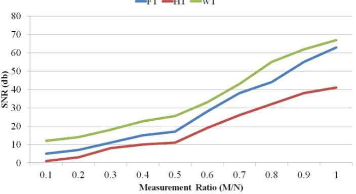
We analyse the effect of HT, WT (including Haar WT, Symlet WT, Coiflet WT, and Daubichi WT), and FT on the signal reconstruction accuracy. In order to compare the signal reconstruction accuracy, we use two metrics: SNR and normalized root mean square error (NRMSE). Figure 9illustrates the comparison between HT, WT and FT in terms of SNR.
Figure 9.Comparing HT, WT, and FT in terms of SNR
Figure 10.Comparing HT, WT, and FT in terms of signal reconstruction error
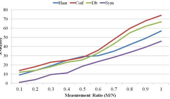
Because WT shows the best performance, we further analyze a number of transforms sub-types. Figure11illustrates the comparison between Haar WT, Symlet WT, Coiflet WT, and Daubichi WT. As we see, most of the time Coiflet WT performs the best in terms of signal reconstruction error (measured as NRMSE) and SNR. Symlet WT performs the worst. However, when the measurement ratio is between 0.3 and 0.5, Haar WT shows better performance.
Figure 12. Comparing Haar WT, Symlet WT, Coiflet WT, and Daubichi WT in terms of signal reconstruction error
8.3. Comparing Distributed and Individual Compressive Sensing
The first part of the performance evaluation section investigates and compares distributed compressive sensing and individual compressive sensing approaches.
Typical signals measured by wireless sensor networks are sparse signals consisting of a common sparse component and different innovation components. Reconstructing these sorts of signals using joint sparse signal recovery models is more efficient than individual signal recovery models. It ultimately reduces the energy consumption and prolongs network lifetime.
For this simulation, we change the number of common and innovative parts. As depicted in Figure
13, distributed compressive sensing provides accurate reconstruction with fewer measurements. On the other hand, increasing the number of common sparsity parameters provides better reconstruction accuracy. When the number of the common sparsity level is minimized, its performance approaches that of a separate compressive sensing method.
Figure 13.Reconstruction accuracy in terms of different common sparsity levels
8.4. Comparing with Other Compressive Sensing based Methods
temporal belief-propagation based compressive sensing (TBCS)[14], OMP based compressive sensing [15] and spatial Bayesian compressive sensing (SBCS)[16].
8.4.1. Data Accuracy
In order to measure the data accuracy, we first compare the accurate reconstruction percentage for the different data compression values. As Figure14indicates, our approach provides accurate data reconstruction with a minimum number of measurements. The main reason for this performance is the value of information gained using the coalition-formation method. Our approach tries to group sensor nodes based on their sparsity similarity, which leads to transmitting more information with a lower number of measurements. However, increasing the compression ratio decreases the gap between our approach and other methods. On the other hand, our approach adjusts the number of measurements based on the signal sparsity level, which removes redundant data transmission. As seen in Figure14, for more compression ratios the reconstruction accuracy is almost the same.
Figure 15.Reconstruction accuracy percentage for different SNRs
transmissions. The number of sensor nodes participating in data transmission is used to measure the number of transmissions. Figure16represents the number of transmissions for different compression techniques by changing number of sensor nodes.
Figure 16.Number of data transmission versus number of sensor nodes
For a network with a lower number of sensors, our approach has a minimum number of transmissions, but this number is comparable with STBCS and SBCS approaches. As the number of sensor nodes increases, the difference in the number of transmissions becomes more significant. This graph also demonstrates the scalability of our method. Our approach localizes sensor nodes based on the similarity of their sparsity levels in separate coalitions. For each coalition, it then curtails the number of transmissions by lessening the number of active sensor nodes participating in data transmission and adjusting the number of measurements to the sparsity level. Therefore, our approach involves a minimum number of transmissions.
8.4.3. Energy Consumption
Figure 17.Energy consumption
The means of grouping sensor nodes and gathering measurements from each group are the main difference among these methods. Since our approach groups the sensor nodes with reference to sparsity similarity, the number of active nodes is diminished. Moreover, it adjusts the number of measurements to the sparsity level, which removes the redundancy in data gathering. STBCS uses a clustering approach to group sensor nodes, but its grouping mechanism is not as accurate as that of our method. In addition, it does not consider adaptability to the number of measurements. Moreover, TBCS, BCS and OMP do not include localization of data gathering, which leads to greater exhaustion of energy .
8.4.4. Trade-off between Energy and Accuracy
We study the trade-off between network energy usage and data accuracy. To do so, we investigate energy consumption in terms of normalized network lifetime, while for accuracy we consider the error between the reconstructed data and real data.
As we can see in Figure18, our approach provides approximately 40% network lifetime at a minimum error level, while with less accurate data it provides higher percentages of lifetime. Adapting both the number of measurements and the number of active sensor nodes to the signal sparsity level is the main contribution of our approach to prolong network lifetime. In addition, spatial-temporal correlation-based coalition formation provides sufficient similarity among sensor node measurements, which leads to less error in the recovered data.
temporal correlation of sensor node readings to achieve an energy efficient data collection. Spatial correlation among sensor nodes and sparsity distribution of signals over the network is used to group sensor nodes in the coalitions. The proposed coalition-formation method is represented by a block diagonal measurement matrix in which each diagonal entity corresponds to one of the coalitions. The localized spatial temporal correlation inside each coalition, builds an efficient measurement matrix which efficiently schedules sensor nodes and balances the data compression and transmission load over the coalition. Upon receiving compressed data in the base station, a two steps belief propagation based signal recovery is implemented to reconstruct the original signal. Having two steps signal recovery allows base station to find the common coefficient of original signal among coalitions and inside coalition. Therefore, it has enough data to recover data per sensor node level, which increases data reconstruction accuracy. Coalition-based data gathering is used to scale down transmission costs, while the number of measurements is minimized by scheduling sensor nodes and adjusting their measurement rate. Our simulation on a real world data set proves our findings and shows more reduction on number of data measurements and compressibility as well as the ability to improve data reconstruction quality.
This paper has also presented a number of transform bases and analyzed their effect on compressive sensing performance in terms of SNR and signal reconstruction error. Since most signals acquired by wireless sensor networks are non-stationary, we considered data collected from bridge monitoring application as a case study for this impact analysis. The comparison of simulation results using FT, HT and WT demonstrates that WT has the best performance when applying compressive sensing to this case study. Coiflet WT, Daubichi WT, Symlet WT, and Haar WT, the sub-families of WT, were also studied and analysed in terms of SNR and NRMSE.
References
1. Rault, T. Bouabdallah, A. Challal, T. Energy efficiency in wireless sensor networks: A top-down survey Computer Networks, Elsevier, 2014, 67, 104-122
2. Leinonen, M. Codreanu,M. Juntti, M. Sequential compressed sensing with progressive signal reconstruction in wireless sensor networks, IEEE Transactions on Wireless Communications, IEEE, 2015, 14, 1622-1635. 3. Balouchestani,M. Raahemifar, K. and Krishnan, T. Robust wireless sensor networks with compressed sensing
theory Networked Digital Technologies, Springer, 2012, 608-619.
4. Middya, R. Chakravarty, M. Naskar, K. Compressive Sensing in Wireless Sensor Networks–a Survey IETE Technical Review, Taylor Francis, 2016, 1-13.
5. Agrawal, A. Ghosh, D. Distributed compressive data gathering in wireless sensor networks Proc. IEEE 11th Int. Conf. Signal Processing, 2012, 3, 2110-2115.
6. Wu, C. Luo, F. Sun, J. Chen, C. W. Efficient Measurement Generation and Pervasive Sparsity for Compressive Data Gathering IEEE Transactions on Wireless Communications, 2010, 9, 3728-3738.
7. Hu, H. Yang, Z. Spatial Correlation-Based Distributed Compressed Sensing in Wireless Sensor Networks Proc. 6th Int. Conf. Wireless Communications Networking and Mobile Computing (WiCOM), 2010, 8. Chen, S. Zhao, C, Wu, M. Sun, Z. Jin, Z. Clustered Spatio-Temporal Compression Design for Wireless Sensor
Networks Computer Communication and Networks (ICCCN), 2015 24th International Conference on, 2015, 1-6
9. Kong, L. Xia, M. Liu, X. Y. Chen, G. Gu, Y. Wu, M. Y. Liu,X. Data loss and reconstruction in wireless sensor networks IEEE Transactions on Parallel and Distributed Systems, IEEE, 2014, 25, 2818-2828.
10. Rashidi, L. Rajasegarar, S. Leckie, C. Nati, M. Gluhak, A. M. Imran, A. Palaniswami, M. Profiling spatial and temporal behaviour in sensor networks: A case study in energy monitoring Intelligent Sensors, Sensor Networks and Information Processing (ISSNIP), 2014 IEEE Ninth International Conference on, 2014, 1-7. 11. Ziniel, J. Schniter, P. Efficient high-dimensional inference in the multiple measurement vector problem IEEE
12. Masiero, R. Quer, G. Rossi, M. Zorzi, M. A Bayesian analysis of compressive sensing data recovery in wireless sensor networks Ultra Modern Telecommunications Workshops, 2009. ICUMT’09. International Conference on, 2009, 1-6.
13. Wu, X. Xiong, Y. Li, M. Huang, W. Distributed spatial-temporal compressive data gathering for large-scale WSNs Proc. Communications and IT Applications Conf 2013 Computing (ComComAp), 2013, 105-110. 14. Shahrasbi, B. Talari, A. Rahnavard, N. TC-CSBP: Compressive sensing for time-correlated data based on
belief propagation Proc. 45th Annual Conf. Information Sciences and Systems, 2011, 1-6
15. Ji, S. Huang, S. Wang, J. Liu, Q. A Reconstruction Method of Compressive Sensing Data Recovery in Wireless Sensor Networks for SHM 2013.
16. Hwang, S. Ran, R. Yang, J. Kim, D. K. Multivariated Bayesian Compressive Sensing in Wireless Sensor Networks IEEE Sensors Journal, IEEE, 2016, 16, 2196-2206.
17. Masoum, A. Meratnia, N. Havinga, P. J. A distributed compressive sensing technique for data gathering in wireless sensor networks Procedia Computer Science, Elsevier, 2013, 21, 207-216.
18. Haupt, J. Bajwa, W. U. Rabbat, M. Nowak, R. Compressed sensing for net- worked data, IEEE Signal Processing Magazine, vol. 25, no. 2, pp. 92–101, 2008.
19. Zhang, Z. Jung, T. P. Makeig, R. Rao, B. D. Compressed sensing of EEG for wireless telemonitoring with low energy consumption and inexpensive hard- ware, IEEE Transactions on Biomedical Engineering, vol. 60, no. 1, pp. 221–224, Jan. 2013.
20. Aderohunmu, F. A. Paci, G. Benini, L. Deng, J. D. Brunelli, D. Swiftnet: A data acquisition protocol for fast-reactive monitoring applications, in Proc. 8th IEEE Int. Symp. Industrial Embedded Systems (SIES), Jun. 2013, pp. 93–96.
21. Luo, C. Wu, F. Sun, J. Chen, C. W. Efficient measurement generation and pervasive sparsity for compressive data gathering, IEEE Transactions on Wireless Communications, vol. 9, no. 12, pp. 3728–3738, Dec. 2010. 22. Hu, H. Yang, Z. Spatialcorrelation-baseddistributedcompressedsensingin wireless sensor networks, in Proc.
6th Int. Conf. Wireless Communications Network- ing and Mobile Computing (WiCOM), Sep. 2010, pp. 1–4. 23. Meng, J. Li, H. Han, Z. Sparse event detection in wireless sensor networks using compressive sensing, in
Proc. 43rd Annual Conf. Information Sciences and Systems, Mar. 2009, pp. 181–185.
24. Yang,X. Tao,X. Dutkiewicz,E. Huang, X. Guo, Y. J. Cui, Q. Energy-efficient distributed data storage for wireless sensor networks based on compressed sens- ing and network coding, IEEE Transactions on Wireless Communications, vol. 12, no. 10, pp. 5087–5099, Oct. 2013.
25. Zheng, H. Yang, F. Tian, X. Gan, X. Wang, X. Xiao, S. Data gathering with compressive sensing in wireless sensor networks: A random walk based ap- proach, IEEE Transactions on Parallel and Distributed Systems, vol. 26, no. 1, pp. 35–44, Jan. 2015.
26. Cheng, L. Niu, J. Kong, L. Luo, C. Gu, Y. He, W. Das, S. K. Compressive sensing based data quality improvement for crowd-sensing applications, Journal of Network and Computer Applications, vol. 77, pp. 123–134, 2017.
27. Candes, E. J. Wakin, M. B. An introduction to compressive sampling, IEEE signal processing magazine, vol. 25, no. 2, pp. 21–30, 2008.
28. Baraniuk, R. Davenport, M. A. Duarte, M. F. Hegde L. An introduction to compressive sensing, Connexions e-textbook, 2011.
29. Haupt, J. Applebaum, L. Nowak, R . On the restricted isometry of deter- ministically subsampled Fourier matrices, in Proc. 44th Annual Conf. Information Sciences and Systems (CISS), Mar. 2010, pp. 1–6
30. Kalogerias D.S. Petropulu, A.P. Ripboundsfornaivelysubsampledscram- bled Fourier sensing matrices, in Proc. 48th Annual Conf. Information Sciences and Systems (CISS), Mar. 2014, pp. 1–6.
31. Baron, D. Duarte, M. F. Wakin, M. B. Sarvotham, S. Baraniuk, R. G. Distributed compressive sensing, arXiv preprint arXiv:0901.3403, 2009.
32. Sundman, D. Chatterjee, S and Skoglund, M. Methods for distributed com- pressed sensing, Journal of Sensor and Actuator Networks, vol. 3, no. 1, pp. 1–25, 2013.
33. Tan, Z. Yang, P. Nehorai, A.Joint sparse recovery method for compressed sensing with structured dictionary mismatches, IEEE Transactions on Signal Pro- cessing, vol. 62, no. 19, pp. 4997–5008, 2014.
34. Haykin, S. Van Veen, B. Signals and systems. John Wiley Sons, 2007.