Loop acoustics with damping

LOOP ACOUSTICS with DAMPING

Matthew Cepkauskas1

1 _{Senior Engineer, GE Oil & Gas, Jacksonville, FL 32221, USA}

Abstract

In a previous SMiRT-20 paper, four one dimensional pipe models with time dependent boundary conditions were developed to be able to predict pump pulsations throughout an acoustic loop. However, this analysis was for pipes containing fluid without acoustic damping. The present paper re-visits the four cases and now includes damping. Series solution convergence is examined to facilitate ease of computations. The problem is one of a non-homogeneous time dependent boundary condition with homogeneous differential equation. The solution is obtained via a transformation technique that introduces additional auxiliary functions. Typically, these auxiliary functions are chosen, but here it is shown that the problem solution is well defined without a choice of auxiliary functions. Numerical results are provided.

INTRODUCTION

Acoustic response of reactor piping and reactor core support structures has a long been addressed at the SMiRT conferences going back to Penzes (1973), Bowers & Horvay (1975) and the present author (1979). Mudaly (2009) examined a method to predict the pump pulsation loading through a complete piping loop. To accomplish this Mudaly considered four cases that represent four different boundary conditions for the one dimensional acoustic model. These cases need to have damping added to them. This is the subject of the present paper.

MATHEMATICAL FORMULATION

The one dimensional acoustic wave equation is given by:



[

P

(

x

,

t

)]



0

, where the operator

2 2 2 0 2

2 2

2 ₁

t C t x

x 

  

 

   

 

 , or alternatively the operator can be given as ₂ 2₂

0 2

2 ₁

t C t

x 

  

   

 



,

both forms of this operator result in the same time dependency in the solution.

Boundary Conditions for case 1, in a complex form: t i p e P t

P(0, ) ₀  (1-a)

0

) , (L t 

P (1-b)

The method of solving this type of problem is found in the work of Fisher et al (1979) and illustrated in several papers by Cepkauskas. It consists of writing a transformation of the form:

t i _p

e P x g t x Q t x

P( , ) ( , ) ( ) ₀  (2)

The differential equation is transformed into a non-homogeneous differential equation: ]

) ( [ )] , (

[ ₀ i pt

e P x g t

x

Q  

 (3)

The boundary conditions become:

t i t

i _{p p}

e P g e P t

] ) ( [ ) ,

( ₀ i pt

e P L g t L

Q   (4-b)

By choosing the following end conditions for g(x), boundary conditions 4-a and 4-b become homogeneous:

) 0 (

g =1 (5-a) g(L)=0 (5-b)

Homogeneous solution:

First set the right-hand side of equation 3 to zero and assume a separable solution in the form of:

)

(

)

(

)

,

(

x

t

X

x

T

t

Q



(6)

results in: 2 2 0 )] ( / ) ( 1 )[ ( ) ( ) ( ) ( _        t T t T t T t T x X x X C   (7)

The spatial dependence becomes:

0

)

(

)

(

₂ 0 2







X

x

C

x

X



(8-a)

With a general solution of the form:

)

sin(

)

cos(

)

(

0 0

x

C

B

x

C

A

x

X









(8-b)

Apply BC’s:

@x= 0

X

(

0

)



A



0

(9-a)

@x=L

(

)

sin(

)

0

L

C

B

L

X





with

L C n n 0







n



1

,

2

,....



(9-b)

The time dependency is of the form:

0

)

(

)

(

)

(

2

2

_

_

_





T



t

T



t



T

t

(10)

Assume a characteristic equation of the form: t

e

t

T

(

)





0

2 2

2

_

_

_

_

_

_

_



(11-a) with

4

4

)

(

2

2 2 2

2

_

_

















(11-b)

Critical damped case:

n crit



2





(12-a) with









_n

/

2

(12-b)

Underdamped case: ) 4 / 1 cos( )

( ₂ 2 2

2

t e

t

T n n

t     _      

(13-a) or () cos( 1 2 )

t e t T n t n     _

  _{  (13-b)}

Forced Response Solution:

The solution to equation 3 is found by assuming a solution of the form:

t i n n p e L x n C t x

Q( , ) sin(  )  1







 (14)

Substitute equation 14 into equation 3, multiply both sides by 2sin( )

0

L x m

C  , integrate over the length

and make use of the orthogonally of the spatial mode shape,

Equation 3 becomes:

dx x g C i x g e L x m C P e i L

C p p

t i L t i p n n p m p

p _{sin( ) { ( )[1 ] ( )}}

] ) [( 2 2 0 2 0 2 0 0 2 2

2 _{  }  _ 

     



     (15)

Consider the integral g x dx

L x m I L ) ( ) sin( 0 





 and integrate by parts twice making use of the boundary

conditions and the restrictions on g(x) given by equation 5. This results in:

dx x g L x m L m L m I L ) ( ) sin( ) ( ) ( 0 2



 

    (16)

Substitute equation 16 back into equation 15 and solve for the set of constantsCn:

] ) [( ] [ 2 ) ( ) sin( 2 2 2 2 2 2 2 0 0 0 0 0 p n n p p n n L m i m i C P dx x g L x m L P C                 

  (17)

substitute equation 17 into 14 and the results into equation 2 results in:

t i n L p e L x n dx x g L x n L P t x

P( , ) 2 sin(  ) ( ) sin(  )  1 00

0      t i t i

n _{p n n p}

p n

n _e p _{g x Pe} p

L x n i n i C

P   

        0

1 2 2 2

2 2 2 0

0 _{sin( ) ( )}

] ) [( ] [ 2         

 (18)

It is easy to prove that the first term is a Fourier expansion of the third term and these terms cancel. This proof consists of multiplying both terms by the spatial mode shape and integrating resulting in an identity. This leaves the solution as simply:

t i

n _{n n}

p e L x n i n i P t x

P  

Where

n p n _

 . After separating the real and imaginary parts the final solution is:

) cos( ) sin( ) 2 ( ) 1 ( 4 1 2 ) ,

( _{2 2 2}

2 2

1

0  _{ }

          

 L t

x n n P t x P p n n (20-a)

 

             _

 tan 2

1 2

tan 1

2

1

_(20-b)

This solution reduces to the Mudaly Case 1 solution when the damping equals zero. Also, note that the time dependency response is identical to that of a spring mass subjected to a base excitation.

This can be further modified to be in the form of the Mudaly solution by letting

L x  

and

0 C Lp  

and

thus

  n   ) cos( ) sin( ) 2 ( ) ( 4 2 ) ,

( _{2 2 2 2}

2 2 2

1

0 _{  }

           

 n n t

P t x P _p n

(21)

The term in the numerator under the square root is approximately 1.0 for small damping and for driving frequencies seen in a PWR, thus the final solution can be approximated as:

) cos( ) sin( 2 ) ,

( _{2 2 2}

) 2 ( ) 1 ( 1 1

0 _{  }

         

 n t

m P t x P p n n (22)

The following is a table from Mudaly and is updated for damping.

TABLE 1 Boundary Conditions, Natural Frequencies and Mode Shapes Case Left Boundary

Condition

0 @x

Right Boundary Condition L x @ Natural Frequen cies Mode Shapes Series indices “j”

1

_P

_x

_t

_P

_t

p



cos

)

,

(



₀

P

(

x

,

t

)



0

L C j



₀

L x j

sin 1,2,3...

2

_P

_x

_t

_P

_t

p



cos

)

,

(



_{0 B t}

x t x P p



cos ) , ( _   L C j 2 0



L x j 2

sin  1,3,5...

3

t

A

x

t

x

P

p



cos

)

,

(

_





t

B

x

t

x

P

p



cos

)

,

(

_





L

C

j



0

L

x

j



cos

0.1.2.3 4

t

A

x

t

x

P

p



cos

)

,

(

_





P

(

x

,

t

)



0

L C j 2 0



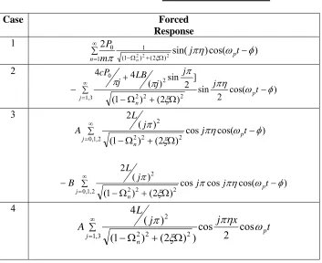
L x j 2

TABLE 2 Series Solution

Case Forced Response

1

) cos(

) sin( 2

2 2 2_{) (2 )} 1

( 1 1

0 _{  }

     



 j t

m P

p

n n

2



 _{  } 

 

3 ,

1 2 2 2

2 0

) cos(

2 sin ) 2 ( ) 1 (

] 2 sin ) ( 4 4

j p

n

t j

j j LB j cP

   

 



3



0,1,2 _2 2_{ } 2  2

) cos(

cos ) 2 ( ) 1 (

) ( 2

j p

n

t j

j L

A   

 



 _{  } 



2 , 1 ,

0 2 2 2

2

) cos(

cos cos ) 2 ( ) 1 (

) ( 2

j p

n

t j

j j

L

B    

 

4



1,3 _2 2_{ } 2

2

cos 2 cos ) ) 2 ( ) 1 (

) ( 4

j p

n

t x

j j

L

A









NUMERICAL RESULTS

Consider the following one dimensional pipe geometry of Length, L=100 inch, C0=20,000 in/sec, P0=1.0

psi, ωp=k*2*π*100 rad/sec where k=1 produces first mode resonance and k=2 produces second mode

resonance and k=1.5 produces a driving frequency half way between the first and second mode (Non-Resonance). This is the same example as in Thanjekwayo (2008).

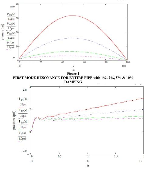
Figure 1 shows the first mode resonance at various damping values. Figure 2 gives the pump end convergence for various damping values. Figure 3 provides the convergence of the solution for a variety of terms in the series near the pump end.

One of the key ingredients in the Mudaly Solution is that an explicit simple function of x is found in the text by Jolley (1961). This reduces the number of unknown constants for a pipe loop to a reasonable number and Crammer’s rule is then used to find the unknows for an entire pipe loop. For the damped case, such an explicit function cannot be found. Figure 5, gives an attempt to determine this function for case 1 based on the known undamped case. The numerical results look identical. However, as in the undamped cases of Mudaly, one can equate the series and exact solution, multiply through by the mode shape, use orthogonality and demonstrate the identity to be correct. When one does the same for the equation given in Figure 5, the identity is shown to be incorrect. Thus, Figure 5 is close to determining the converging function of x, but comes up short.

This is an interesting problem that must be resolved. Typically, a function of x is known and then we can use Fourier analysis to obtain the series coefficients, mode shapes and resulting series representation. Here we have the reverse problem in that we have the coefficients, mode shapes and resulting series but do not have the function.

Figure

1

FIRST MODE RESONANCE FOR ENTIRE PIPE with 1%, 2%, 5% & 10%

DAMPING

Figure 2

Figure 3

CONVERGENCE OF SOLUTION AT RESONANCE

with 1%, 2%, 5% & 10%

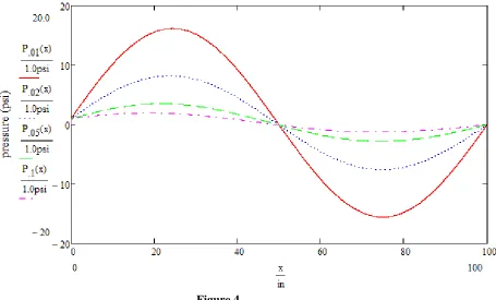
AT PUMP END WITH VARIOUS NUMBER OF TERMS IN SERIES

Figure 4

Figure 5

ATTEMPT TO OBTAIN JOLLEY SERIES CONVERGENCE

Figure 6

Figure 7

AMPLITUDE VERSUS K FOR X=0.5L & X=0.25L

CONCLUSIONS

Damping has been added to the four cases needed to perform a complete one dimensional pipe loop acoustic analysis. Numerical results are provided. A future problem of identifying the series convergence identity will be pursued in the future.

REFERENCES

Bowers, G. and Horvay, G. , “Forces of a Shell Inside a Narrow Water Annulus”, 3rd _{International}

Conference on Structural Mechanics in Reactor Technology, London, United Kingdom, September 1-5, 1975, Paper F 2/8.

Cepkauskas M.M., “Acoustic Pressure Pulsations in Pressurized Water Reactors”, 5th _{International}

Conference on Structural Mechanics in Reactor Technology, Berlin, Germany, August 13-17, 1979. Cepkauskas M.M. and Thanjekwayo, Ronald, “PBMR PCU Acoustics”, Flow Induced Vibration Conference, FIV 2008, Prague, Czech Republic, July 1-4, 2008

Fisher H. D, Cepkauskas M.M. and Chandra, S., “Solution of Time Dependent Boundary Value Problems by the Boundary Operator Method”, International Journal of Solids and Structures, 1979, volume 15, pp. 607-614.

Jolley L.B.W, 1961 Summation of Series. New York, Dover Publications

Penzes, L.E. “Theory of Pump Induced Pulsating Coolant Pressure In Pressurized Water Reactors”, 2nd

International Conference on Structural Mechanics in Reactor Technology, Berlin, Germany, September 10-14, 1973, Paper E 5/1*.