Application of evolutionary computing in the design of high throughput digital filters.

(1)

University of Windsor University of Windsor

Scholarship at UWindsor

Electronic Theses and Dissertations Theses, Dissertations, and Major Papers

1-1-2007

Application of evolutionary computing in the design of high

throughput digital filters.

Payman Samadi

University of Windsor

Follow this and additional works at: https://scholar.uwindsor.ca/etd

Recommended Citation Recommended Citation

Samadi, Payman, "Application of evolutionary computing in the design of high throughput digital filters." (2007). Electronic Theses and Dissertations. 6989.

https://scholar.uwindsor.ca/etd/6989

This online database contains the full-text of PhD dissertations and Masters’ theses of University of Windsor students from 1954 forward. These documents are made available for personal study and research purposes only, in accordance with the Canadian Copyright Act and the Creative Commons license—CC BY-NC-ND (Attribution, Non-Commercial, No Derivative Works). Under this license, works must always be attributed to the copyright holder (original author), cannot be used for any commercial purposes, and may not be altered. Any other use would require the permission of the copyright holder. Students may inquire about withdrawing their dissertation and/or thesis from this database. For additional inquiries, please contact the repository administrator via email

(2)

A p p lica tio n o f E v olu tion ary C o m p u tin g in

th e D esig n o f H igh T h rou gh p u t D ig ital

F ilters

by

P a y m a n S am ad i

A Thesis

Subm itted to the Faculty of G raduate Studies and Research

through Electrical and Com puter Engineering

in P artial Fulfillment of the Requirements for

the Degree of M aster of Applied Science at the

University of Windsor

Windsor, Ontario, Canada 2007

(3)

Library and Archives Canada

Bibliotheque et Archives Canada

Published Heritage Branch

395 W ellington Street Ottawa ON K1A 0N4 Canada

Your file Votre reference ISBN: 978-0-494-35014-0 Our file Notre reference ISBN: 978-0-494-35014-0 Direction du

Patrimoine de I'edition

395, rue W ellington Ottawa ON K1A 0N4 Canada

NOTICE:

The author has granted a non exclusive license allowing Library and Archives Canada to reproduce, publish, archive, preserve, conserve, communicate to the public by

telecommunication or on the Internet, loan, distribute and sell theses

worldwide, for commercial or non commercial purposes, in microform, paper, electronic and/or any other formats.

AVIS:

L'auteur a accorde une licence non exclusive permettant a la Bibliotheque et Archives Canada de reproduire, publier, archiver,

sauvegarder, conserver, transmettre au public par telecommunication ou par I'lnternet, preter, distribuer et vendre des theses partout dans le monde, a des fins commerciales ou autres, sur support microforme, papier, electronique et/ou autres formats.

The author retains copyright ownership and moral rights in this thesis. Neither the thesis nor substantial extracts from it may be printed or otherwise reproduced without the author's permission.

L'auteur conserve la propriete du droit d'auteur et des droits moraux qui protege cette these. Ni la these ni des extraits substantiels de celle-ci ne doivent etre imprimes ou autrement reproduits sans son autorisation.

In compliance with the Canadian Privacy Act some supporting forms may have been removed from this thesis.

While these forms may be included in the document page count,

their removal does not represent any loss of content from the thesis.

Conformement a la loi canadienne sur la protection de la vie privee, quelques formulaires secondaires ont ete enleves de cette these.

Bien que ces formulaires aient inclus dans la pagination, il n'y aura aucun contenu manquant.

i*i

Canada

(4)

erwise retain ed in a retreival system or tra n sm itte d in any form, on any m edium by

any means w ithout prior w ritten perm ission of th e author.

(5)

Abstract

In this thesis, th e application of E volutionary C om puting in th e design of high

thro u g h p ut digital filters is studied. E volutionary Com puting are a group of problem

solving m ethods which are based on biological evolution, such as n a tu ra l selection

and genetic inheritance. From these problem -solving techniques, Genetic A lgorithm

(GA) and Im m une Program m ing (IP) are chosen for Digital Filter design application.

We sta rt th is research by developing iterativ e design methodologies for Finite Im

pulse Response (FIR) and Infinite Im pulse Response (HR) 1-D filters and also FIR

and IIR Q u ad ratu re M irror F ilter (Q M F) banks. T he proposed methodologies con

sider phase linearity as another co n strain t for th e design formulation. Several studies

on th e perform ance analysis of G enetic A lgorithm are performed. T he dependence

of M ean Square Error (MSE) on populatio n size and num ber of generations were in

vestigated. The perform ance of GA over different cross-over techniques and different

values for probability of cloning (Pc) an d probability of m utation (Prn) is analyzed

too.

Furtherm ore to ob tain high th ro u g h p u t ra te digital filters, Common Subexpression

Elim ination (CSE) is applied on th e coefficients. In th is thesis, th e existing algorithm

for 2 non-zero digits CSE in b o th vertical and horizontal position is extended to 3

iv

(6)

A B S T R A C T

non-zero digits for vertical elimination. At the end, a new algorithm for th e design of

high th ro u g h p u t digital filters w ith CSE constraint, linear phase characteristics and

Canonical Signed Digit (CSD) coefficients is proposed which leads to more efficient

digital filters.

R eproduced with perm ission of the copyright owner. Further reproduction prohibited without perm ission.

(7)

To My Family.

vi

(8)

Acknow ledgments

I would like to express my sincere gratitu d e and appreciation to Dr. M ajid A hm adi,

my supervisor, for his invaluable guidance throughout the course of th is thesis work.

Special th a n k s to Dr. Kemal Tepe, Dr. Huapeng Wu. Dr. Shervin Erfani and Dr.

Esam A bdel-R aheem for th eir expert guidance and constant support thro u g h o ut my

study. I would also like to th an k Dr. W. A bdul-K ader for reviewing this work.

I also sincerely appreciate my family for th eir endless support and my friends for th eir

help and friendship.

vii

(9)

C ontents

A b stract iv

D ed ica tio n vi

A cknow ledgm ents vii

List o f Figures xii

List o f Tables x v

List o f A b b reviation s xvii

1 Introd u ction 1

1.1 Digital F i l t e r s ... 2

1.1.1 One-Dimensional F i l t e r s ... 2

1.1.2 Q u ad ratu re M irror F ilter B a n k s ... 3

1.2 CSD C o d in g ... 6

1.3 Sum m ary of Previous W o r k s ... 8

1.4 Thesis O b je c tiv e s ... 9

1.5 Thesis O rg a n iz a tio n ... 9

2 E volu tion ary C om p u tin g 10 2.1 I n tr o d u c tio n ... 10

viii

(10)

C O N T E N T S

2.2 G enetic A lgorithm ... 11

2.2.1 G enetic A lgorithm C y c l e ... 11

2.2.1.1 Problem C o d i n g ... 13

2.2.1.2 Fitness F u n c t i o n ... 13

2.2.1.3 R e p ro d u c tio n ... 13

2.2.1.4 C r o s s o v e r ... 15

2.2.1.5 M u t a t i o n ... 17

2.2.1.6 Replacem ent ... 17

2.2.2 E x a m p le ... 17

2.2.3 GA A n a ly sis ... 22

2.2.3.1 Effect of R e p ro d u c tio n ... 22

2.2.3.2 Effect of C ro s s o v e r... 23

2.2.3.3 Effect of M u t a t i o n ... 23

2.2.3.4 Schema G rowth E q u a t i o n ... 24

2.2.4 Effect of Crossover and M utation on CSD n u m b e r ... 24

2.3 Im m une P r o g r a m m in g ... 26

2.3.1 Im m une S y s te m ... 26

2.3.1.1 P a tte rn R e c o g n itio n ... 26

2.3.1.2 Clonal Selection A lgorithm ... 27

2.3.2 Im m une P r o g r a m m in g ... 29

2.3.3 E x a m p le ... 37

2.4 C o n c lu sio n ... 40

3 C om m on S u b ex p ressio n E lim ination 41 3.1 I n tr o d u c tio n ... 41

3.2 Different S u b e x p re s s io n s ... 42

3.2.1 H orizontal Subexpression E lim in a tio n ... 42

3.2.2 V ertical Subexpression E l i m i n a tio n ... 43

ix

(11)

C O N T E N T S

3.3 Design P r o c e d u r e ... 44

3.3.1 Identification G raph ... 44

3.4 Common vertical subexpression for 3 non-zero d ig its ... 50

3.4.1 Search G r a p h ... 54

3.4.2 Exam ple W alk Through th e Search G r a p h ... 56

3.5 Elim ination using GA ... 56

3.6 E xperim ental R e s u lts ... 57

3.7 C o n clu sio n ... 58

4 Form ulation o f D ig ita l F ilter D esig n using E volu tion ary C o m p u tin g 59 4.1 I n tr o d u c tio n ... 59

4.2 Design of digital filters using G A ... 60

4.2.1 General Design F l o w ... 60

4.2.1.1 I n i t i a l i z a t i o n ... 60

4.2.1.2 Fitness e v a l u a t i o n ... 61

4.2.1.3 R e p r o d u c tio n ... 63

4.2.1.4 C r o s s o v e r ... 63

4.2.1.5 M u t a t i o n ... 63

4.2.1.6 CSD C h e c k ... 63

4.2.1.7 Replacem ent S t r a t e g y ... 63

4.2.2 Different Coding T e c h n iq u e s ... 64

4.2.2.1 Technique 1 (Ternary C o d in g )... 64

4.2.2.2 Technique 2 (New Coding S c h e m e ) ... 65

4.2.3 Experim ental Results and th e Com parison of th e Two Coding Scheme ... 66

4.2.3.1 F IR filters w ith te rn a ry CSD c o d i n g ... 66

4.2.3.2 H R filters w ith te rn a ry CSD c o d in g ... 69

4.2.3.3 F IR filters w ith new CSD coding s c h e m e ... 70

X

(12)

C O N T E N T S

4.2.3.4 H R filters w ith new CSD coding s c h e m e ... 73

4.2.3.5 F IR filters w ith linear phase characteristic and new CSD coding scheme ... 74

4.2.3.6 H R filters w ith linear phase characteristic and new CSD coding scheme ... 77

4.2.3.7 C om parison of Two Coding S c h e m e s ... 79

4.2.4 Perform ance A nalysis of G A ... 83

4.2.4.1 Effect of population size and num ber of generations on M S E ... 83

4.2.4.2 Perform ance of GA on different crossover techniques 85 4.2.4.3 Effect of Pc and Pm on M S E ... 85

4.3 Design of D igital F ilter w ith I P ... 87

4.4 New A lgorithm for D igital F ilter D e s i g n ... 90

4.4.1 E x a m p le ... 92

4.5 C o n c lu sio n ... 94

5 C onclusion 95

R eferen ces 98

V IT A A U C T O R IS 103

xi

(13)

List o f Figures

1.1 T he two-channel Q M F B an k... 4

1.2 C om parison of CSD and B inary M u ltip lic a tio n ... 7

2.1 Search Techniques... 12

2.2 GA Cycle... 12

2.3 R oulette W heel Selection... 15

2.4 1-point Crossover... 16

2.5 2-point Crossover... 16

2.6 Uniform Crossover... 17

2.7 Effect of Crossover on CSD coefficients... 25

2.8 Effect of M utation on CSD coefficients... 25

2.9 P a tte rn Recognition w ith B-cells and T-cells... 27

2.10 Clonal Selection A lgorithm ... 28

2.11 Flow chart of th e IP algorithm [31]... 36

3.1 G raph of Vertices... 46

3.2 P artial Identification G raph G'id... 47

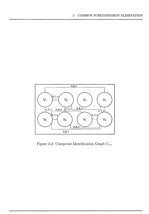
3.3 C om peted Identification G rap h Gid... 49

3.4 G raph of Vertices... 51

3.5 P artial Identification G raph G\d... 52

3.6 C om peted Identification G rap h Gid... 54

xii

(14)

L IS T O F F IG U R E S

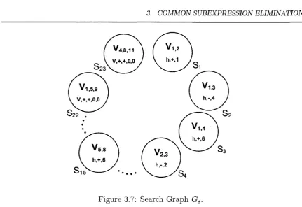
3.7 Search G raph G s... 55

4.1 GA Design Flow... 61

4.2 19th order, low-pass F IR filter w ith 16 bit CSD coefficients and m axi m um 4 non-zero digits (Ternary C o d i n g ) ... 67

4.3 5th order, low-pass H R filter w ith 16 b it CSD coefficients and m axim um 4 non-zero digits (Ternary Coding) ... 69

4.4 19th order, low-pass F IR filter w ith 16 bit CSD coefficients and m axi m um 4 non-zero digits (new coding scheme) ... 71

4.5 5th order, low-pass HR filter w ith 16 b it CSD coefficients and m axim um 4 non-zero digits (new coding scheme) ... 73

4.6 19th order, low-pass F IR filter w ith 16 bit CSD coefficients and m axi m um 4 non-zero digits (Linear Phase and new coding scheme) . . . . 75

4.7 Phase C haracteristic of 19th order, low-pass FIR filter w ith 16 bit CSD coefficients and m axim um 4 non-zero digits (Linear Phase and new coding s c h e m e ) ... 76

4.8 5th order, low-pass HR filter w ith 16 b it CSD coefficients and m axim um 4 non-zero digits (Linear Phase and new coding scheme) ... 77

4.9 Phase C haracteristic of bth order, low-pass HR filter w ith 16 b it CSD coefficients and m axim um 4 non-zero digits (Linear Phase and new coding s c h e m e ) ... 78

4.10 Com parison of two techniques for H R f i l t e r s ... 81

4.11 Com parison of two techniques for F IR f i l t e r s ... 82

4.12 Effect of population size and num ber of generations on M S E ... 84

4.13 M ean Square Error vs. Pc ... 86

4.14 M ean Square E rror vs. Pm ... 86

4.15 IP Design Flow... 87

4.16 5th order HR F ilter Designed using IP ... 88

xiii

(15)

L IS T O F FIG U RES

4.17 Common Subexpression Elim ination for a 19th order FIR filter using IP. 89

4.18 The Proposed Fitness Function... 91

4.19 5th order HR filter designed w ith th e new a l g o r ith m ... 93

xiv

(16)

List o f Tables

2.1 S u b to tal of Chromosomes’ F it n e s s ... 19

2 . 2 In stru ctio n Set [ 3 1 ] ... 30

3.1 Coefficient S ta c k in g ... 46

3.3 Edge List E'id for 2 non-zero digits {a = 1, 2 ,..., 8, b = 1 ,2 ,..., 8 } . . . 48

3.5 Vertices and th eir p r o p e r tie s ... 51

3.6 Edge List E'id for 2 non-zero d ig its ... 53

3.7 Edge List E'id for 3 vertical non-zero d i g i t s ... 54

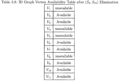
3.8 ID G rap h Vertex Availability Table after (S3, S1 5) Elim ination . . . . 57

3.9 CSE on F IR f i l t e r ... 58

4.1 Conversion Table For CSD Length = 6 ... 6 6 4.2 CSD Coefficients of th e 19th order low-pass FIR filter w ith tern ary coding 6 8 4.3 B inary Coefficients of th e 5th order low-pass HR filter w ith tern ary c o d i n g ... 70

4.4 B inary Coefficients of th e 19th order low-pass FIR filter w ith new cod ing s c h e m e 72 4.5 B inary Coefficients of the 5th order low-pass HR filter w ith the new coding s c h e m e ... 74

XV

(17)

L IS T OF TA B LE S

4.6 Com parison for HR Q M F Bank O rder 5 ... 80

4.7 Com parison for F IR QM F B ank O rder 19 ... 80

4.8 MSE for 3rd, 5th and 7th order H R filter w ith different cross-over tech

niques ... 85

4.9 CSD coefficients of 5th order HR f i l t e r ... 92

xvi

(18)

List o f Abbreviations

l-D One-dim ension

2-D Two-dim ension

AIS A rtificial Im m une Systems

ASIC A pplication Specific Integrated Circuits

CSD C anonical Signed Digit

CSE Com m on Subexpression Elimination

Cl C om p u tatio n al Intelligence

DSP D igital Signal Processing

E Set of G rap h Edges

FDM Frequency Division M ultiplexing

FIR F inite Im pulse Response

FPS fitness p ro po rtio n ate selection

G G raph

GA G enetic A lgorithm

ID Identification

HR Infinite Im pulse Response

IP Im m une Program m ing

LP Linear Phase

Pc P rob ab ility of Cross-over

Pm P ro b ab ility of M utation

Pi P rob ab ility of Inversion

QM F Q u a d ratu re M irror Filter

TDM Tim e Division M ultiplexing

TSP Traveling Salesm an Problem

xvii

(19)

C hapter 1

Introduction

Interests on discrete tim e signals have been enormously increased during past three

decades. In discrete tim e signals, error correction is much easier and higher transm is

sion rates can be achieved. Digital Signal Processing (DSP) is a field of engineering

th a t works on th e discrete tim e signals. D SP has a wide range of applications, from

home devices such as DVD players and TV tuners to precise biom edical devices (Mag

netic Resonance Im aging (M RI)) and in security applications such as face and iris

recognition.

One im p o rtan t branch of DSP is Digital Filters [36]. D igital Filters work on

discrete tim e d a ta and basically perform digital m athem atical operations on them .

These d a ta can be one-dimension (1-D), two-dimensions (2-D) [47] or in general N-

dimensions (N-D). As an example, 1-D signal can be audio signal, 2-D signal can be

image of a scene and 3-D signal can be a video.

1

(20)

1. IN T R O D U C T IO N

1.1 D ig ita l F ilte r s

D igital Filters are an im p o rtan t p a rt of Digital Signal Processing. T hey can be used

signals and for restoring th e disto rted signals. As an example when we have an audio

signal which is co rrup ted w ith th e high frequency noise, a low-pass filter w ith the

cut-off frequency of 20K H z can cut the unw anted noise.

D igital Filters m ay be im plem ented in software or hardw are. Software implemen

ta tio n can be a software on a general-purpose com puter and hardw are im plem entation

can be a DSP chip or an ASIC processor.

Similar to discrete tim e d ata, Digital Filters can be in one-dimension (1-D), two-

dimensions (2-D) and in general in N-dimensions (N-D) [40]. In this section different

kinds of (1-D) digital filters are reviewed.

1.1 .1

O n e -D im e n s io n a l F ilte r s

1-D digital filter can be in th e form of FIR (non-recursive) or H R (recursive) and can

be characterized by th e ir difference equation. A linear, tim e-invariant F IR filter can

be shown as:

By using th e z-transform , a digital filter can be described in z-dom ain which is

helpful in frequency dom ain analysis. In theory, th e transfer function of a digital

filter is th e z-transform of its impulse response. T he transfer function of a linear,

tim e-invariant F IR filter is defined as:

for different applications b u t in general they are utilized for separating th e combined

N

(1.1) i=0

N

(1.2)

2

(21)

The same form ulation is also available for HR filters. A linear, tim e-invariant HR

filter can be shown as:

N M

y(n ) = a (i )x (n - ^ - ^ 2 b(*)y(n - *) (i-3)

i = 0 i= 1

And its transfer function can be shown as:

H (z ) = -.f - r (!-4)

In th e digital filter design we are always interested to have stable filters. F IR filters

are always stable therefore th ere is no need for stability check, b u t for H R filters

stability check should be perform ed. The poles of th e tran sfer function determ ine

w hether th e filter is stable or not. In E quation 1.4, th e denom inator polynom ial D( z )

must satisfy th e following constraint:

D( z ) ^ 0 \/\z\ > 1 (1.5)

By this constraint all poles of th e D( z ) are located inside th e u n it circle of z plane,

therefore th e filter is stable. For stability check we have used th e Jury-M arsden [40]

m ethod which does not require finding any polynom ial roots and only requires th e

calculation of th e determ inant of a series of 2 by 2 m atrices.

1.1 .2

Q u a d r a tu r e M irro r F ilte r B a n k s

Q uadrature M irror F ilter (Q M F) banks have been subject of research for many

years [48]. They are applied for th e situation where a discrete-tim e signal x[n] is

needed to be split into a num ber of sub-band signals Xj[n] so th a t each can be pro

cessed separately. Typical processing comprises down-sampling, coding for tra n s

mission and storage. Subsequently at some point, these signals are needed to be

recombined together to have th e original signal reconstructed. T he m ost common

3

(22)

\ [ n ]

-x i f n j _{y,[n ]}

Figure 1.1: T h e two-channel QMF Bank.

applications are frequency dom ain speech samplers, sub-band coders for speech sig

nals and digital trans-m ultiplexers used in Frequency Division M ultiplexing (FDM )

/ Time Division M ultiplexing (TD M ) conversion.

Based on th e type of synthesis and analysis filter (FIR or HR) and num ber of

channels, there are different kinds of filter banks. In this research we have focused

on 2-channel QM F bank for b o th F IR and IIR. Fig. 1.1 shows th e basic two-channel

QM F bank. The analysis filter b an k is composed of a low-pass filter H0( z) and a high

pass filter H\ ( z) . These tw o filters split th e incoming signal to two frequency bands.

The sub-band signals are th e n dow n-sam pled by a factor of two. Each down-sam pled

sub-band signal is encoded by exploiting th e special spectral properties of th e signal,

such as energy level and p e rcep tu al im portance. At the receiving end these signals

are up-sam pled by a factor of two and fed into the tw o-band synthesis filter bank

Gq(z) and G'i (z). and at th e end th e o u tp u t is created by adding these two signals.

Up-sam pling of xo[n\ an d x\[n] result in images, which have to be elim inated by

G0(z) and Gi (z). The o u tp u t of G0(z) and G\{z) are a good approxim ation of x0[n]

and X i[n], and th e reco n stru cted signal y[«] closely resembles x[n). In Q u ad ratu re

M irror F ilter banks th e response of H0(z) is the m irror image of th e response of H\ (z).

In Fig. 1.1 th e relation betw een th e in p u t and o u tp u t signal is [40]:

(23)

Y ( z ) = ± G 0( z ) H0(z) + Gi { z ) Hi ( z ) + ± G 0( z ) H0( - z ) + G l { z ) Hl { - z ) x { - z ) (1.6)

In order to have an alias-free QM F bank , we should set these two filters in a such

way th a t aliasing effect be canceled; this will lead to Linear Tim e Invariant (LTI)

system. Following is th e condition of alias-free QM F bank [40]:

G0(z) = H 1( - z) (1.7)

—Go(—z) = Gi ( z ) (1-8)

H1(z) = H0( - z ) (1.9)

According to th e above equation, by designing Hq(z) only, we will have th e whole

system designed. For FIR Q M F bank th ere is no need for stability check b u t for

H R filters, stability check m ust be carried out for th e designed filters. We have used

th e Jury-M arsden [40] m ethod, which determ ines th e stability by th e calculation of a

series of 2 by 2 determ inants and does not require finding any polynom ial roots. The

N th order real coefficient H R H t)(z) is defined as:

E t=0a ( b > ^ N (Z)

- - M--—— ■ - TT77T (1-10)

E i = o K v z 1 V G )

The group delay of a filter is a m easure of th e average delay of th e filter as a

function of frequency and is defined as:

„ r d H ( z ) / d z , „ r D' (z) N' ( z ) , , 111N

t ( w) = —Re[z 7y (V) ]z = e ^ T = - z - j ^ \ z=ejwT (1.11)

W here D' [ z) = dD^ and N ' ( z) = dN^ .

For the N th order real coefficient FIR filter, Hq(z) is

N

H( z ) = (1.12)

i = 0

(24)

1.2 C S D C o d in g

CSD num ber system is a representation of a num ber as a sum and difference of power

of two.

M

x = ^ 2 s k2~Pk (1.13)

k= 1

W here s k are tern ary digits, s k € 1, 0 ,1 , and I is defined as -1.

M is a pre-specified word length, an d p k G 0 .1 ...., M .

and w ith th e constraint:

sk x Sk+i = 0, for all th e k 6 0 ,1 ,..., M . (1-14)

As an example, we w ant to represent 0.8743 in CSD num ber system. There is

limit of 4 non-zero digits and th e w ord len g th is 8. The CSD representation of 0.8743

is:

0.8743 ~ 2° - 2~3 - 2~7 = 1.0010001

CSD num ber system has advantages over conventional binary system. CSD rep

resentation contains fewer non-zero digits therefore there are less p artial products in

m ultiplications of the num bers. As an exam ple 15 in binary representation is (1111)2

which contains 4 non-zero digits b u t in CSD representation, it is (10001) which has

two non-zero digits. Fig. 1.2 illu strates th e comparison between binary and CSD

m ultiplication. It is shown th a t for th e m ultiplication of 14 and 15 in binary system,

4 additions are needed b u t in CSD form at only 1 subtraction is needed which is the

same as addition.

The m athem atical operations in digital filters are in the form of m ultiplication, ad

dition and shift. In th e im plem entation of digital filters, addition and shift operations

are cheap. W hen a digital filter faces a series of inp u t data, m ultiplication operation

forms as M ultiple C onstant M ultiplication (MCM). M ultiple C onstant M ultiplications

6

(25)

1. IN T R O D U C T IO N 14 x 15 Binary Multiplication 00001110 00001111

00001110 add 00001110 add 00001110 add

00001110 add

0011010010 = (210)

CSD Multiplication 14 00010010

x l 5 00010001 00010010 00010010

subtract

shift 3 times add 00100110010 = (210)

Figure 1.2: Com parison of CSD and Binary M ultiplication

consum e m ost of th e power and im plem entation cost in digital filters.therefore low

im plem entation cost MCM is always desired. One popular m ethod for reducing th e

im plem entation complexity of MCM is to constrain th e coefficients to have canonical

signed digit (CSD) form at w ith lim ited num ber of non-zero digits[ 1 ]. jo]. Thereby th e

heavy MCMs can be replaced by fewer shift and add operation.

By Using th e Common Subexpression Elim ination (CSE) [117]. j:F>], [17], further

reduction can also be made in th e num ber of addition in M ultiple C onstant M ulti

plication. CSE is the process of finding th e common p attern s (subexpressions) in a

expression and calculate th em once and use th e result where the subexpression oc

curs w ithin th e expression. Since removing one subexpression may destroy another

subexpression, it is critical to find th e optim um subexpression for elim ination. As an

exam ple, in th e following expression, choosing th e horizontal subexpression (101) will

destroy th e vertical subexpression (11) and viceversa.

c0 101010101

ci 101000101

7

(26)

1.3 S u m m a ry o f P r e v io u s W orks

Generally there are two approaches for th e design of digital filters, direct [19] m ethod

and indirect [45] m ethod. In indirect m ethod, first a norm alized analog filter using

classical approxim ations m ethods such as B u tterw o rth , Chebychev, Elliptic, etc [40]

is designed, th en through some discretization process, th e desired digital filter is

digitized. Famous discretization procedures are invariant impulse response m ethod,

m atched z-transform ation and bilinear tran sfo rm atio n [40].

In direct m ethod [1], [18], by utilizing iterativ e optim ization m ethods, th e desired

discrete-tim e transfer function is calculated. In these m ethods first a discrete-tim e

transfer function is formed thro u g h an initial guess. T hen th e error function which is

based on th e desired m agnitude and phase response is defined. T he optim al answer

is obtained by minimizing the error function w ith respect to th e coefficients of th e

transfer function.

In all of th e above-mentioned design techniques, coefficients are calculated w ith

high precision b u t in actual im plem entation, either hardw are or software, th e filter

coefficients are stored in finite length registers, so quantization m ust be applied.

Q uantization in digital filters m ay result in u n stable filters a n d /o r different response.

This has resulted in designs w ith finite precision coefficients. Four popular iterative

optim ization techniques are branch and bou n d optim ization [11], discretization and

re-optim ization [30], sim ulated annealing [32] and genetic algorithm [44].

Genetic Algorithm (GA) is a stochastic search m ethod th a t im itates th e process

of n a tu ra l selection and evolution. GA possesses m any features such as parallelism

and m ultiple objectivity and filters designed by GA have th e potential of obtaining

near global optim um solution [25]. D uring th e p ast decade, GA has been successfully

used to design digital filters [33], [12], [16]. Also th e utilization of CSD coefficients

has th e advantage of minimizing th e im plem entation cost of digital filters.

In literatu re there are several proposed techniques for th e design of digital filter

8

(27)

using genetic algorithm [27], [26], [18], [1], [23] b u t none of th em has th e Common

subexpression Elim ination as a factor in the fitness function. In this thesis we propose

a new algorithm , which include characteristics such as M agnitude Response, Phase

Linearity and Common Subexpression Elim ination in its objective function. We also

have extended th e existing algorithm for common subexpression elim ination to 3

non-zero digits in vertical position.

1.4 T h e sis O b jec tiv es

T h e work presented in this thesis conforms to th e following objectives:

1. Study th e application of th e evolutionary com puting such as GA and IP in th e

design of digital filters.

2. Perform a thorough study on perform ance of Genetic A lgorithm for digital filter

design.

3. Develop a new algorithm for th e design of high th ro u g h p u t D igital Filter.

4. E x ten d th e Common Subexpression Elim ination to 3 non-zero digits.

1.5 T h e sis O rg a n iza tio n

T his thesis is organized as follows: C hapter 2 covers th e G enetic A lgorithm and

Im m une Program m ing. C hapter 3 presents th e Common Subexpression Elim ination

and its extension to 3 non-zero digits for vertical subexpressions. C h ap ter 4 is th e

form ulation for D igital F ilter design using Evolutionary C om puting and th e proposed

algorithm and lastly, C hapter 5 provides concluding remarks.

(28)

C hapter 2

Evolutionary Computing

2.1 In tr o d u c tio n

Evolutionary C om puting [6] is a group of problem solving m ethods which are based

on biological evolution, such as n a tu ra l selection and genetic inheritance. Prom these

m ethods Artificial Neural Networks [39], Genetic A lgorithm [50] and Artificial Im

mune Systems [7] can be nam ed. Each of these m ethods is inspired from a biological

process of hum an body i.e. Artificial N eural Networks are inspired from th e neural

system of th e body, Genetic A lgorithm is inspired from th e m echanism of n atu ral

evolutionary genetics and Artificial Im m une System is inspired from th e Immune

System of hum an body. In this chapter two of these paradigm s, G enetic A lgorithm

and Artificial Imm une Systems, are discussed.

10

(29)

2. E V O L U T IO N A R Y C O M P U T IN G

2.2 G e n e tic A lg o r ith m

Genetic A lgorithm (GA) is a search and optim ization algorithm which is based on

mechanism of n a tu ra l evolutionary genetics. It was developed by Jo h n Holland [20]

in 1975 in his ’’A d a p tatio n in N atural and Artificial Systems” and was further im

proved by G oldberg [14], [15] and others [22]. This m ethod works on a population

of candidate solutions and tries to find th e optim al answer.

GA is based on th e m echanism of n atu ral selection and th e principal of survival of

th e fittest. In th is algorithm , individuals in a population com pete for survival. After

each generation th e m ost successful individuals are more likely to survive and th e less

successful individuals are gradually eliminated.

For solving real-w orld problems w ith Genetic A lgorithm , th e solution to th e prob

lem m ust be expressed as a character string called chromosomes. Also there should

be a fitness function to determ ine th e fitness of individuals. In th e process of GA, it

tries to ob tain a b e tte r solution from the existing solutions.

As it was m entioned GA is a search-based optim ization technique. Search tech

niques can be divided into th ree groups, random search, enum erative and calculus

based. Fig. 2.1 shows different search techniques.

2 .2 .1

G e n e t ic A lg o r ith m C y c le

Genetic A lgorithm cycle by G oldberg [15] is shown in Fig. 2.2. This algorithm consists

of three operations: R eproduction, Crossover and M utation.

Chromosomes of each population which are th e candidate solutions are fed into

th is cycle. There m ust be a fitness function defined for each problem to determ ine

th e fitness of each solution. R eproduction selects th e fitter chromosomes from each

population for crossover and m utation. New population is created by each cycle and

this process is rep eated until th e minimum error or m axim um num ber of generations

11

(30)

2. E V O L U T IO N A R Y C O M P U T IN G

Search Techniques

i i

-C a lc u lu s

B a s e d R a n d o m E n u m e r a tiv e )

Sim u lated A nealing

D irect Indirect ) R an d o m W alk

N e w to n 's M ethod Z ero G radiant Evolutionary Algorithm

E volutionary S tra te g ie s

G en etic A lgorithm s

A S e q u e n tio n a l

Figure 2.1: Search Techniques.

Population

Reproduction Mutation

Cross-Over

Figure 2.2: GA Cycle.

is achieved. The chromosome th a t has th e highest fitness is th e solution to th e targ et

problem.

A G enetic A lgorithm in its simplest form operates as th e following steps:

1. G enerating th e random initial population.

2. Evaluating th e fitness of each chromosome.

3. Selecting a group of chromosomes as parents.

12

(31)

4. C reating new p o pu latio n by crossover and m utation.

5. Replacing th e new pop u latio n according to its fitness.

6. R epeating th e loop to reach th e target.

In th e following sections, each of these steps is discussed in detail.

2.2.1.1 P ro b lem C o d in g

Encoding scheme [2] is th e link betw een real-world problem and th e G enetic Algo

rithm . T he solution of th e problem m ust be encoded to form th e chromosomes and

each chromosome is a possible solution for the problem. Chromosome consists of

string of a characters which can be in binary, integer or any other form at.

Encoding of th e problem is a crucial issue. Inappropriate coding can intensively

lim it th e searching space w hich may lead to non-optim al results. The length of th e

chromosome is also a m ajo r factor in Genetic Algorithm. According to th e problem

in hand, long or short chromosomes may lead to b e tte r results [34].

2.2.1.2 F itn ess F u n ction

The fitness function is a n o th er link of Genetic A lgorithm to th e real-world problem.

Every problem m ust have an objective function to evaluate th e chromosomes. The

higher fitness m eans th e b e tte r result.

At th e s ta rt of th e GA, after creating the initial random population, th e fitness

of each chromosome is evaluated and th en fed into th e GA loop for reproduction.

2.2.1.3 R ep ro d u ctio n

R eproduction is th e process of random ly selecting chromosomes w ith respect to their

fitness. Regardless of repro d u ctio n mechanism, a chromosome w ith a higher fitness

will have a higher probability of being chosen. This is the sim ulation of survival-of-the

13

(32)

fittest in n a tu ra l selection process in which any organism which is m ore fit will have

a b etter chance to survive in nature.

There are m any approaches [49], [51] for reproduction operation such as rank

selection, fitness proportionate selection (FPS) and tournam ent selection. All of these

approaches try to give m ore chances to fitter chromosomes to be selected as parents.

A common F P S m ethod is R oulette W heel Selection. The idea of R o u lette W heel

Selection is to divide th e wheel to non-uniform slots w ith respect to chrom osom es’

fitness. A chromosome w ith higher fitness will have a bigger slot. W hen th e wheel

is spun, th e chromosome w ith th e highest fitness has the great est chance of being

chosen. The wheel is spun till th e whole population is created. In this m eth o d some

chromosomes m aybe tak en more th a n once. R oulette W heel executes th e following

steps:

1. Sum th e fitness of all Chromosomes.

2. G enerating random num ber between 0 and to ta l fitness.

3. Choose th e chromosome whose fitness added to th e fitness of th e proceeding

chromosomes is less or equal to random number.

4. R epeat th e steps till th e population size is reached.

Fig. 2.3 is an example of R oulette W heel Selection. Assume th at th ere are three

chromosomes: 01010, 11110 and 11001 w ith th e fitness value of 40(Z. 35% and 19%

of the to ta l fitness. For creating th e population, R oulette W heel is spun th re e tim es

and in each spin one of th e chromosomes is selected. Chromosome 01010 has th e

46% of th e to ta l fitness, therefore it has th e greatest chance of being selected. In th e

Roulette W heel Selection, one chromosome can be selected more th a n once.

(33)

Chromosome 3 I 19%

Chromosome 1

46% Chromosome 2 35%

Figure 2.3: R oulette W heel Selection.

2 .2.1.4 C rossover

The selected individuals from th e reproduction will be used as parents for crossover.

Crossover is th e m ain operato r for exploring th e searching area. In this operation,

according to a probability ra te which is Probability of Crossover (Pc), two new chro

mosomes are generated. As th e probability increases, GA can explore more diversity

of th e solution space b u t if th e Pc is to o high, the high fitness chromosomes may

destroy [29].

There are variety of crossover operators [21], [43], [38] such as one-point, 2-point

and n-point crossover operator. In th e following sections, these th ree approaches will

be discussed.

1. 1-point Crossover

In single point cross-over [10], a cross-over point is chosen a t a random position

between 1 and th e (st rin g length —1). Two new chromosome strings are created

by dividing th e initial chromosome strings into two sections each at th e cross

over point and appending th e first half of the first chromosome string to th e

second half of th e second chrom osome string and vice versa.

15

(34)

Figure 2.4: 1-point Crossover.

2. 2-point Crossover

2-point cross-over [4] has chromosomes arranged in loops by joining th eir ends

together. Two cuts are m ade in the loop and the resulting segments are ex

changed. From th is it can be seen th a t 1-point is ju st a special case of th e more

general 2-point cross-over where one of th e cut points is fixed as falling betw een

th e last and first position.

Figure 2.5: 2-point Crossover.

3. N-point Crossover

A nother form of crossover is th e n-point crossover [42] where th e num ber of

points n varies dynam ically w ith each m ating. In th is m ethod, a random ly

generated crossover m ask is used to determ ine which genes of an offspring come

from which parent. Each gene in th e first offspring is created by copying th e

corresponding gene from one or th e other parent according to th e crossover

mask. W here th ere is a 1 in th e mask, th e gene is copied from th e first parent,

and where th ere is a 0 in th e mask, th e gene is copied from th e second parent.

The process is repeated w ith th e parents exchanged to produce th e second

offspring. A new crossover m ask is random ly generated for each pair of parents.

16

(35)

0 1 0 1 1 0 0

Figure 2.6: U niform Crossover.

2.2.1.5 M u ta tio n

Normally, m utatio n [41] occurs w ith low probability and functions as a background

operator. Assume th a t A = 101010101 is th e chromosome and 1 is th e chosen bit

for m utation according to th e probability of m u tatio n Pm. As there are to ta ly three

possibilities for strings (1 ,1 ,0 ), 1 m ust be changed random ly w ith I or 0. If it is

changed w ith 0, th e new chromosome will be A = 101000101.

2.2.1.6 R ep lacem en t

Elitist strategy [24] is applied for th e replacem ent of old generation. A fter th e fitness

evaluation, if th e m axim um fitness of old population is less or equal to th e maxim um

fitness of new population, it is replaced by th e new population.

2 .2 .2

E x a m p le

Having introduced th e G enetic A lgorithm an d its operators, now there is an example

to dem onstrate th e GA. In th is problem we w ant to find th e m aximum of f { x ) = x ‘2—x

where 1 < x < 5.

S te p l. Variable Coding:

In this problem, variable x is coded as a 5 b it binary num ber, so a random guess

17

(36)

can be x = 1 0 1 1 0 which is x = 2 2.

Step2. Initialization:

In this step, a population size of chromosomes are random ly generated to initialize

th e population. Here we have used 6 as th e population size, so th e initial population

can be:

ax = [10110] = 22

g2 = [00011] = 3

a3 = [11011] = 27

a4 = [00101] = 5

a5 = [11110] = 30

a 6 = [01000] = 8

Step3. Fitness Evaluation:

In this problem we w ant to find th e m axim um of f ( x ) = x2 — x when 1 < x < 5.

T h e function value f ( x ) is a good candidate for th e fitness function, f i t n e s s = f ( x ) =

2

X — X.

f i t n e s s ( a 1) = /(2 2 ) = 462

fitness(a,2) = /(3 ) = 6

f i t n e s s (as) = /(2 7 ) = 702

f i t n e s s ( a f ) = /(5 ) = 20

f i t n e s s ( a5) = /(3 0 ) = 870

f i t n e s s ( a 6) = / (8) = 56

Step4. Reproduction:

1 8

(37)

R oulette W heel Selection is our approach for reproduction operation. Here is the

steps:

1. C alculate th e to ta l fitness.

6

F — f it n e s s ( a j) — 2116. i=i

2. G enerate a random num ber in th e range of [0, 2116]. As an example one can

choose th e generated num ber as 2103.

3. Select a chromosome based on th e su b to tal of chromosom es’ fitness and random

generated number.

Table 2.1 shows th e su b to tal of chrom osom es’ fitness in this problem.

Table 2.1: Subtotal of Chrom osom es’ Fitness

Chromosomes Sum of th e Proceeding Fitness

f i t n e s s ( a i ) = 462 462

f i t n e s s ^ ) = 6 468

f i t n e s s ( a3) = 702 1170

fitness{a±) —2 0 1190

fitness(a,5) = 870 2060

fi tne ss( ae) = 56 2116

According to th e Table 2.1 and th e num ber 2103, Chromosome a5 is selected.

4. R epeat steps 2 and 3 to select th e oth er chromosomes as parents. We assume

th a t th e five selected chromosomes are as follow:

o' = a5 = [11110] = 30

1 9

(38)

a2 = a5 = [11110] = 30

a'3 = a i = [10110] = 22

a'4 = a3 = [11011] = 27

a'5 = a5 = [11110] = 30

ag = a 6 = [01000] = 8

Step5. Crossover:

C reating new population starts by crossover. In this example one point crossover is

used an d th e probability of crossover is 85%. Following is th e procedure for crossover:

1. Select two chromosomes randomly. Chromosomes a2 and a'4 are selected.

2 . G enerate a random num ber between [0, 1]. Random generated num ber is 0.543.

3. Since 0.543 < P c, crossover operation is performed. Select a crossover point

random ly betw een [1,5]. 3 is selected as crossover point, so a2 and a3 exchange

genes after th e crossover point.

4. R epeat steps 1-3 until th e population size is complete. In this case 6 chromo

somes are created.

a’[ = [11111] = 31

a" = [1 1 0 1 0] = 26

a" = [1 0 1 1 0] = 2 2

a!{ = [11011] = 27

a’l = [01111] = 15

a" = [11000] = 24

20

(39)

Step6 . M utation:

M utation perform s on b its w ith th e probability of 0.05. E ach b it of each chromo

some is exam ined w ith th e Pm and if th e random generated num ber is less th a n Pm,

m utation is applied. A fter m utatio n th e new chromosomes are as follows:

Cl =

c2 =

C3 =

c4 =

C5 =

C6 =

[10111] = 23

[1 1 0 1 0] = 26

[1 0 0 1 0] = 18

[11011] = 27

[11111] = 31

[11000] = 24

Step7. Fitness E valuation and Replacem ent:

f i tn e s s ( c i) = 506

f i t n e s s ( c2) = 650

f i t n e s s ( c3) = 306

fi tn e s s ( c i) = 702

f i t n e s s ( c5) = 930

f i t n e s s ( c6) = 552

After step7, first generation of genetic algorithm is com pleted. For next generation

we continue step 4 to step 7 till reach th e m axim um num ber of generations. The

best chromosome of th e final generation is th e optim al answer. In this example

chromosome {11111} = 31 is th e m axim um of /(:/;) when 1 < :r < 5.

21

(40)

2 .2 .3

G A A n a ly s is

In this section we w ant to analyze th e effect of Genetic A lgorithm operators such as

R eproduction, Crossover and M utation. For th is purpose th e notion of schem ata [14]

has to be introduced. Schem ata is a string composed of the letters of th e chromosomes

(1, 0 for binary) and * for th e d o n ’t care position. A schema represents all strings

which m atch all th e positions except *. For example for a binary string of length 5,

th e schem ata *0 1 1* m atches chromosomes 1 0 1 1 0, 0 0 1 1 0 and 0 0 1 1 1.

2.2.3.1 Effect o f R ep ro d u ctio n

Assume th a t th e average fitness of th e schema h is m(h, t) and £(h, t ) be th e num ber

of m atched chromosomes by th e schema h in th e current generation. If R oulette

W heel Selection is used as th e reproduction operator, th e num ber of chromosomes

th a t m atch schem a h can be estim ated in the next generation [46]:

C ( M + 1) = C ( M ) x (2 . i )

which M (t ) is th e average fitness in th e current generation. Let

_ m(h, t) — M( t ) .

M( t ) 1 ‘ ’

if e > 0 , it m eans th a t in th e current generation, th e schema has an above-average

fitness. S u b stitu tin g E quation 2.2 in E quation 2.1, we will have

C (M + l) = C ( M ) x ( l + e) (2.3)

S tarting from t = 0, we will o b tain th e equation

£(h, t + 1) = £(h, 0) x (1 + e f (2.4)

22

(41)

E quation 2.4 shows th a t after reproduction operation, th e above-average schema

will receive an exponentially increasing num ber of chromosome in th e next generation

and th e below-average schema will die.

2.2.3.2 Effect o f C rossover

In th e crossover operation, schema survives only if th e crossover po in t falls outside

of th e schema i.e if th e length of th e chromosome is L, and 5(h) is th e order of the

schema h, h survives only if th e point is outside of its defining len g th 6(h).

For th e one-point crossover, th e probability of distortion of strin g h is [46]:

P d ( h ) = (2.5)

therefore th e probability of th e survival of schema h is [46]:

p s(h) = 1 - (2.6)

Assuming th a t Pc is the probability of crossover, th en th e probability of schema

survival is:

P8C(h) > 1 - Pc (2.7)

E quation 2.7 shows th a t as th e order of th e schema increases, th e probability of

th e survival of the schema decreases.

2.2.3.3 Effect o f M u ta tio n

M utation works in b it level w ith a low probability which is called probability of

m utatio n (Pm). The probability of a single bit to survive is 1 — Pm. A schema

survives from distortion only if all th e positions in th e schema rem ains unchanged.

The form ulation for th e probability of a schema h surviving th e m u ta tio n operation

is [46]:

2 3

(42)

P s ( h ) = (1 ~ P m ) m (2.8)

In genetic algorithm Pm <C 1, so Equation 2.8 can be approxim ated as

(2.9)

E quation 2.9 shows th a t for high order schema, distortion is more probable.

2 .2 .3 .4 S chem a G row th E q u ation

If we combine the effect of reproduction, crossover and m utation, we will ob tain the

following schema grow th equation [46]:

E quation 2.10 shows th a t schem ata w ith short, above-average and low-order prop

erties receive exponentially increasing num ber of representatives in th e subsequent

generations of a GA, therefore th e encoding scheme of th e problem m ust be chosen

in a way th a t these kind of schem ata be produced.

2 .2 .4

E ffect o f C r o sso v e r a n d M u ta tio n o n C S D n u m b e r

Crossover and M utation operations m ay violate th e CSD form at. These two opera

tions can create invalid coefficients by breaking the two constraints of CSD num ber

system. They can violate th e non-zero adjacency constraint by p u ttin g two non-zero

digits besides each oth er or increase th e num ber of non-zero digits to more th a n pre

specified limit. Fig. 2.7 shows th e effect of crossover on CSD num ber an d Fig. 2.8

shows th e effect of m u tatio n on CSD form at chromosomes. In chapter 4 we present

two different techniques to overcome this problem.

(2.10)

24

(43)

l

Dt (CSD Parent) 1 o !l 0 0 1 0 1

i i

D2 (CSD Parent) 0 1 jO 0 1 0 0 1

l

f

j Crossover point D*i (Invalid offspring) Q 1 0 1

D* 2 (CSD offspring) 1 0 0 0 1 0 01

Figure 2.7: Effect of Crossover on CSD coefficients.

D, (CSD Parent) 1 0 1 0 0 1 0 1 Bit Mutation

D*i (Invalid offspring) fi 1 1K) 0 1 0 1 i ____I

Figure 2.8: Effect of M utation on CSD coefficients.

25

(44)

2.3 Im m u n e P r o g r a m m in g

Artificial Im m une System (AIS) [7] is a search and optim ization technique which

is inspired by th e im m une system of th e body and its principles and mechanisms.

Imm une program m ing (IP) [31] is a novel paradigm combining th e program -like rep

resentation of solutions to problem s w ith th e principles and theories of th e immune

system. Basically, IP is th e extension of th e Clonal Selection A lgorithm in Artificial

Imm une Systems. IP is not dependent to any dom ain and it can be applied on a wide

variety of problems.

2 .3 .1

Im m u n e S y s te m

The immune system [9] of th e b o d y is a n atu ral, rapid and effective defence mechanism

for our body to work against infections. Knowing th a t artificial neural networks are

inspired from th e nervous system of th e body, similar to th a t, th e immune system

has led to th e emergence of artificial im m une systems as a com putational intelligence

(Cl) paradigm .

The immune system consists of two stages of defence which are th e innate immune

system and th e adaptive im m une system . T he innate immune system works through

th e cells th a t are always available. T hey defend against th e wide range of bacteria

and they d o n ’t need any pre-knowledge of them . The adaptive im m une system pro

duces th e antibodies only in response to specific infections. These cells have memory

therefore th ey are capable to recognize th e same infection when it is presented to th e

organism again.

2.3.1.1 P a tte r n R eco g n itio n

Lym phocytes which are th e com ponents of th e white blood cells, are th e tools for the

p a tte rn recognition in Im m une System. Lym phocytes are in two types, B-cells and

26

(45)

T-cells. B oth of these two elements have receptors for identifying th e antigens b u t

B-cells can recognize th e isolated antigen from th e outside and T-cells can recognize

th e antigenic cell complex. Fig. 2.9 shows th e difference of these two elements.

The process of p a tte rn recognition is based on m atched shapes. W hen a T-cell

or B-cell receptor com pliments th e antigen, th e recognition is perform ed. T h ere is a

concept affinity which is th e degree of binding between the receptors and th e cell.

B-celi receptor

T-cell

receptor

Figure 2.9: P a tte rn Recognition w ith B-cells and T-cells.

2.3.1.2 C lonal S election A lgorithm

The Clonal Selection Algorithm (CSA) [8] is th e base of Im m une Program m ing. It

is th e theory th a t describes the operation of adaptive immune system. A ccording to

this theory, only th e cells which have th e capability of recognizing th e antigen can

proliferate and th e rest are discarded. It works on b o th B-cells and T-cells w ith some

difference. In CSA B-cells suffer som atic m u tatio n [8] during reproduction b u t T-cells

d o n ’t suffer m utation during reproduction.

Fig. 2.10 shows th e principle of Clonal Selection Algorithm. In th is figure darker

circles have the higher fitness and th e inner circles in step 3 represent th e level of

27

(46)

m utation.

Fig. 2.10 illustrates th a t after initialization, cells w ith successful binding are

cloned. This will lead to a new population. T he new population will be m u tated

w ith respect to th eir fitness to make a new cell w ith a slight difference. Due to th e

high m u tatio n rates, th is process is usually called hyperm utation. This whole process

of selection and hyperm utation is called clonal selection.

n candidate solutions are generated and their fitness is evaluated

©

Candidates with high fitness is selected for cloning (rate is proportional to their fitness )

©

N ew ly Generates Clones are subjected for mutation (rate is inversely proportional to their fitness )

Figure 2.10: Clonal Selection Algorithm.

In summary, th e m ain properties of th e clonal selection algorithm are:

• A ntibody generation

• R eproduction for high affinity antibodies

• M utation w ith respect to affinity

2 8

(47)

2 .3 .2

Im m u n e P r o g r a m m in g

T h e IP algorithm is the development of Clonal Selection A lgorithm and th e replace

m ent of low affinity antibodies. IP consists of th e following steps:

1. Initialization

2. Evaluation

3. Replacem ent

4. Cloning

5. H yperm utation

6 . Iteration-repertoire

7. Iteration-algorithm

S te p l. Initialization:

In th is step, th e initial repertoire of antibodies are random ly generated. In IP

antibodies can be instruction sets for th e problem. Table 2.2 is a sample instruction

set which is taken from the [31]. Each instruction is coded and th e greatest code

num ber has th e value of r — 1, where r is th e num ber of instructions in th e instruction

set.

N ext step is choosing th e length of th e program . The length of th e program can

be variable or fixed. For variable length program s, nop instruction can be used as

padding. For th e program length hardw are constraints should be tak en into account

as well. As an example according to th e Table 2.2 , th e a ttrib u te string of m = < 1,4 >

represents: du p add

29

(48)

Table 2.2: In stru ctio n Set [31]

Instruction Code D escription

nop 0 No operation

dup 1 D uplicate th e to p of th e stack (x —» x x₎

swap 2 Swap th e to p two elem ents of th e stack (x y -- + y x )

m ult 3 M ultiply th e to p two elem ents of th e stack (2 4 —> 8 )

add 4 A dd th e to p two elem ents of th e stack ( 2 4 ■- 6 )

over 6 D uplicate th e second item on th e stack (x y —> y x y )

The program length L and th e size of in stru ctio n size r state th e available anti

bodies for th e problem. Here we sta rt w ith one exam ple to show th e different steps

of th e algorithm .

In th is exam ple th e length of th e program is 5 and th e size of th e repertoire

n — 100. Let us consider th e following antibodies from th e whole repertoire. These

antibodies are th e possible solution for th e problem . The notatio n A B is reserved

for th e whole repertoire and th e notatio n Abi is reserved for each antibody in the

repertoire.

Abx =< 2 ,4 ,5 ,1 ,0 >;

Ab2 = < 1 ,3 ,0 ,5 ,0 >;

Abs —< 5,1, 5, 2 ,4 >;

Ab4 =< 4 ,3 ,2 ,1 ,0 > .

Step2. Evaluation:

A ntibodies are th e possible solution for th e problem and th e antigen is th e prob

lem. A ntigen can be represented in different form ats. In th is example the antigen is

an arithm etic expression [31].

30

(49)

Ag = x2 + x + x y

N ext all of th e antibodies are decoded and th e corresponding program s are taken

out. T h en th e whole repertoire is com pared w ith th e antigen and th e affinity is

calculated.

Pgi = swap add over dup mult;

P9 2 = dup m ult nop add nop;

P g3 = over nop over swap add;

P( / 4 = over m ult swap dup nop.

To evaluate th e affinity of th e antibodies numerical argum ent values m ust be

generated and p u t into th e stack to get the value. These argum ent can be generated

random ly w ithin a prescribed range. In this example argum ent are restricted to 1-byte

integer [0,..., 255]. 4 sets of random argum ents are generated as x = [123, 58, 241, 22]

and y = [7,36,124,263],

The results of executing the antibodies Abi are

P si= [130, 94, 365, 285];

P g 2=[15136, 3400, 58205, 747];

P p 3= [ 130, 94, 365, 285];

P # 4=[105903, 121104, 7202044, 127292],

Symbol N /A is reserved for th e program s th a t failed to re tu rn a result. The

antigen A g yields th e values [16113, 5510, 88206, 6292].

Affinity is calculated using the distance between th e generated program Pgi and

th e antigen A g, th e n th e three-tiered measure is added. The three tired-m easure are:

E x cita b ility . If th ere is no error after program running, it is assigned a score Tf.

31