Importance sampling methodologies for simulation of communication systems with time-varying channels and adaptive equalizers

Importance Sampling Methodologies

for Simulation of Communication

Systems with Time-Varying

Channels and Adaptive Equalizers

Wael

A.

Al-Qaq

Michael Devetsikiotis

J.

Keith Townsend

~,,---..: , ./ . \ '- C. <:»;...

r r:r ..r-'-"" ....

',z., \ ,/ /

\ \.,,_ /4i' i

\, ~ .'.."~'

'~C"

,.-".,.0'

Center for Communications and Signal Processing,

Department of Electrical and Computer Engineering

North Carolina State University

To appear (with revisions) in the IEEE Journal on Selected Areas in Communications

Importance Sampling Methodologies for Simulation

of Communication Systems with Time-Varying

Channels and Adaptive Equalizers

Wael A. AI-Qaq, Student Member IEEE Michael Devetsikiotis, Student Member IEEE

J.

Keith Townsend, Member IEEE

Center for Communications and Signal Processing, Department of Electrical & Computer Engineering, North Carolina State University, Raleigh, NC 27695-7914

Abstract

Formula-based analysis of communication links with time-varying channels and adaptive

equalizers is not always tractable - Monte Carlo simulation must be used to obtain bit error

rate (BER) estimates of the system. Conventional Monte Carlo simulation will not provide

estimates for low BER's due to excessive run time. Although importance sampling (IS)

techniques offer the potential for large speed-up factors for BER estimation using MC sim-ulation, IS techniques have not been used for simulating communication links with adaptive equalizers.

In this paper we present, for the first time, two IS methodologies for MC simulation of communication links characterized by time-varying channels and adaptive equalizers. One methodology is denoted here as the "twin system" (TS) method. A key feature of the TS method is that biased noise samples are input to the adaptive equalizer, but the equalizer is only allowed to adapt to these samples for a time interval equal to the memory of the system.

In addition to the TS technique, we also present a statistically biased, but simpler tech-nique for using IS with adaptive equalizers which is based on the independence assumption between the equalizer input and the equalizer taps (the "IA" method).

Experimental results are presented that show run time speed-up factors of two to seven orders of magnitude for a static linear channel with memory, and of two to almost five orders of magnitude for a slowly varying, random linear channel with memory, for both the IA and

TS methods.

1. This research was sponsored in part by an IBM Fellowship.

2. Portions of this paper have been presented at the IEEE GLOBECOM'92, Orlando, Florida, December

Importance Sampling Methodologies ... , Al-Qaq, Devetsikiotis, & Townsend

1

Introduction

1

~erfo~mance

analysis of digital communication links characterized by time-varying channels

IS a difficult problem. The recent flurry of interest in wireless mobile communications has

also increased the importance of this problem. In these links, adaptive equalizers are used

to track the time-varying channel and ensure satisfactory performance

[1,

2]. Formula-based

analysis of these links is not always possible - Monte Carlo simulation must be used to

obtain bit error rate (BER) estimates of the system. Depending on the complexity of these

systems, Monte Carlo simulation can provide accurate BER estimates of a time-varying

system with an adaptive equalizer down to approximately 10-4 • Although this may be

sufficient for many voice-band applications, in the future these networks will require lower error rates, thus exceeding the capabilities of conventional Monte Carlo simulation.

Importance sampling (IS) techniques offer the potential for large speed-up factors for BER estimation using MC simulation [3,4,5,6]. However, IS techniques have not been used

to speed-up

Me

simulation of communication links with adaptive equalizers. Appropriate

IS parameter values must be used, since poor choices for these parameters could even

re-duce simulation efficiency, resulting in slow-down instead of speed-up. In the past, we have

presented methods for locating near-optimal IS parameter values for the simulation of static

communication channels [7, 8].

In addition to formulation problems, the use of IS in MC simulation of adaptive systems during the training period (i.e., the initial period when the actual data transmitted is fed back to the adaptive equalizer to help it correctly track channel variations) is faced with the difficulty that the adaptive system will attempt to undo the effect of the IS biasing scheme. A necessary requirement of any good IS biasing scheme is that the scheme causes a significant increase in the "raw" (i.e., unweighted) BERof the system. Since we are primarily concerned with the performance of adaptive equalizers in the period subsequent to the training period, and since adaptive equalizers adjust to force theBERtoward zero during the training period, our IS technique is applied to the adaptive system in the period that follows the training period. During this period, the output decisions are fed back to update the equalizer taps and track channel variations.

A fundamental complication in finding an appropriate IS methodology is the fact that adaptive systems possess a cumulative memory that extends back to time zero. The delete-rious effects of large memory on IS are well known. Also, the adaptive equalizer taps, and thus the optimal IS parameter values, are a function of time.

In this paper we present, for the first time, two IS methodologies for

Me

simulation of

communication links characterized by time-varying channels and adaptive equalizers. One is denoted here as the "twin system" (TS) method. A key feature of the TS method is that biased noise samples are input to the adaptive equalizer, but the equalizer is only allowed to adapt to these samples for a time interval equal to the memory of an equivalent system model. The memory for this equivalent system model remains constant. At the end of this interval a decision is collected. The adaptive equalizer taps are then reset to values which

would have resulted had there been no IS. A new optimal

IS

biasing value for the next vector

Importance Sampling Methodologies ..., Al-Qaq, Devetsikiotis, & Townsend 2

Embodied in the TS technique is a novel simulation model consisting of the "original system" and a "twin system". The original system keeps track of the equalizer taps variation with time with unbiased noise samples. Biased noise samples are applied to the twin system.

Also,

Me

statistics (using IS) are measured at the output of the twin system. Equalizer tap

values are transferred from the original system to the twin system at the beginning of each biasing cycle.

The chief contribution of this paper is to present the theoretical foundation for the TS and IA estimators and demonstrate the potential of these techniques with examples. Keep in mind that it is not possible to calculate the exact BER using closed-form analysis even for a static linear channel with an adaptive equalizer.

To formulate the TS method, it was necessary to develop an equivalent system model which combines memory elements on both the analog and digital sides of the decision op-eration into one equivalent system. The equivalent system model was derived for the LMS

algorithm, but the TS and IA methodologies presented in this paper are applicable to all

adaptive algorithms with differences merely in the details of developing an equivalent system model.

In addition to the TS technique, we also present a method for using IS with adaptive equalizers which is based on the independence assumption between the equalizer input and the equalizer taps. This "IA" method has clear implementation advantages over the twin system method, but yields a statistically biased estimator, with the bias increasing with the amount of correlation between the input data and taps. The assumption of independence between the input and equalizer taps is widely used in literature on adaptive systems (see [9] and references within). Furthermore, and most importantly, our experimental results also support this assumption and demonstrate that the IS estimator based on the IA method offers significant speed-up factors, while its relative statistical bias with respect to the "correct" TS estimator is acceptably small. Thus the IA estimator provides an alternative approach, and could be especially useful for cross-checking and validation.

The details of the equivalent system are presented in Section 2. The twin system and

independence assumption methods are formulated in Section 3. Experimental results

pre-sented in Section 4 show run time speed-up factors of two to seven orders of magnitude for a

static linear channel with memory, and of two to almost five orders of magnitude for a slowly varying, random linear channel with memory for both the IA and TS methodologies. The overhead of the TS technique is modest, reducing the net speed-up by roughly a factor of 2 for a 6-tap equalizer, and a factor of approximately 3.5 for a lO-tap equalizer. The proof of a result useful for selecting biasing parameter values is given in the Appendix.

2

Formulation

2.1

Adaptive Systems Model

Fig. 1 shows the block diagram of a digital communication system in which a linear adap-tive equalizer is used to compensate for the distortion caused by the transmission medium

Importance Sampling Methodologies _{... ,} Al_-Qaq_,eveD isiki ii & rt: d

51 0 18, .LOWn5en ₃

Transmitter

p(t)

Time-Varying ChannelWith

Memory

----..I

a(t) --'

Gaussian Noise (Unbiased)

Receiver Filter

Figure 1: .Block diagram of a digital communication system which includes a time-varying channel with memory and an adaptive equalizer.

whose output is given by

00

a(t)

==

L

akP(t -

kT,I ) 1e=0

where

i,

is the bit rate in the system. The channel

z(., t)

distorts the transmitted signal

a(t)

and causes intersymbol interference (lSI). The signal

s(t)

is given by

s(t)

==

z(a(t),t)

The signal coming out of the channel is corrupted by additive noise, which is usually wide band Gaussian noise. The resulting signal at the input to the receiver is given by

x(

t)

==

s(

t)

+

n(

t)

The output of the (linear) receiver is sampled once every bit interval (i.e. every Tilseconds) to obtain

y(

k) ==

x(

t)

*

q(

t)

It=1eT.

In addition to the distorted transmitted symbol, the output signal

y(k)

contains intersymbol

interference due to channel distortion, as well as additive noise.

Let the equalizer be an FIR filter (tapped delay line) with M adjustable taps, hi (k), i ==

0, ...

,M -

1, at every time

k.

The equalizer output may be expressed as

M-l

ak

==

L

hm(k)y(k -

m)

m=O

There are different algorithms for updating the equalizer taps with time k. These algorithms

vary in performance, complexity, and applications. The mean square error (MSE) at instant

k is given by

M-l

MSE(k)

==

E{e 2(k)}

== E{(a1e - alc)2}

=

E{(alc -

L

hm(k)y(k -

m))2}

m=O

Importance Sampling Methodologies ..., Al-Qaq, Devetsikiotis, & Townsend 4

algorithm, but the general

Me

and IS formulations of sections 2.3 and 2.4 with our IS

methodologies of section 3 are applicable to all adaptive algorithms with differences merely in the details of finding the equivalent system model.

According to the LMS algorithm, the search for the minimum MSE is done using the gradient descent technique. For real valued data signals, the corresponding update equation for the equalizer taps is given by

h(k)

==

h(k - 1)

+

JLe(k -

l)y(k - 1)

where

h (k)

==

[ho(k ), h1 (k ), ... , hM-1 (k )] and

y(k)

==

[y(k),y(k -

1),... ,y(k - M

+

1)]

Furthermore,

e(

k)

==

ale -

ak

where

JL

is the step size, with 0

<

JL

<

2/[MPyy(O)]

[1].

Pyy(O)

is the power in the signal

y(k)

that is easily estimated from the received signal.

2.2

Equivalent Syst ern Model

In order to develop a model of our adaptive system suitable for use with IS, we need to

express the final output

ak

as a function of the random inputs

x(l), I

== 0, ... ,

k,

to the

receiver filter. This function must have components in both the analog and the digital parts of the receiver, posing certain modeling difficulties. We overcome these difficulties as follows:

Let M1 be the channel memory in bits. Let M2be the receiver filter memory in bits. Denote

the receiver filter taps by

q

==

[q1'

'Iz»> • •,QM2L]

where L is the number of samples per bit. Let S, N, and X denote the 1 X

M

vectors of

bit-length vectorss(i), n(i), and x( i), respectively, defined as follows:

S(k)

==

[s(k)

I

s(k -

L)

I ... I

s(k -

(M -

I)L)]

s(i)

==

[.s(i), ... , .s(i -

L

+

1)],

i ==

k, k - L, ... , k -

(M -

l)L

N(k)

==

[n(k)

I

n(k - L)

I ... I

n(k - (M - l)L)]

n(i) ==

[n(i), ... ,n(i -

L

+

1)],

i

==

k,k -

L, ...

,k -

(M

-l)L

Then

X(k)

==

S(k)

+

N(k)

==

[x(k)

I

x(k - L)

I ... I

x(k - (M - l)L)]

with

x(i) ==

[x(i), ... , x(i -

L

+

1)],

i

== k, k - L ... , k -

(M -

1)L

Importance Sampling Methodologies ..., Al-Qaq, Devetsikiotis, & Townsend

where

if

=

M

+

M2 - 1bits (corresponding to

M

x L samples),

and A is the

if

L X

M

matrix

5

Observe that, since

y(k)

=

X(k)A,

we have

y(k -

1)

=

X(k - L)A

and

heq(k)

=

heq(k

-1)

+

Ite(k -l)X(k - L)AA

T

(1)

Thus,

heq(k)

is a function of

X(k - L)

and

heq(k -

1).

But

heq(k -

1)

is a function of

X(k - 2L)

and

heq(k -

2)

and so on, therefore we can conclude that

heq(k)

=

g(x(O), ...

,x(k - L))

=

g'(Xc(k -

L),X(k - L))

where g and g' are functionals dependent on A and

It

and

Xc(k)

=

[x(k -

ML)/ .. .

lx(O)]

(2)

is the vector "complementary" to

X(k).

Note that (2) is general in describing the cumulative memory behavior of most adaptive algorithms, where the adaptive equalizer taps at any instant k are a function of the input samples extending

all

the way back to k

=

O.

2.3

Monte Carlo Formulation

For the time-varying communication system in question, the probability of a detection error at any instant k is given by

Pe(k)

E{I(X(k)h~(k))}

J

I( abT) !X(k).heq(k)(a,

b)

da db

1

!z(O)•...,z(k)(eO,. · ·

,ek)deo · .. dek

°X,1t

(3)

where !X(k).heq(k) is the joint probability density function (pdf) of X(

k)

and he q (

k),

!z(O)...z(k)

is the joint pdf of the

x(i)'s,

i

=

0, ... ,

k,

f2X.1c

=

{(x(O), ... , x(k)) :

I(X(k)h~(k))

=

I}

Importance Sampling Methodologies ... , Al-Qaq, Devetsikiotis,

&

Townsend 6

The bit error rate (BER) given by (3) is defined as the instantaneous BER. A Monte

Carlo (MC) estimator of

(3)

is given by the sample mean expression

(4)

where

X(k,i)

and

h;q(k,i)

are i.i.d. repetitions of

X(k)

and

h;q(k),

respectively. Note that

X(k,i)

and

h;q(k,i)

are not independent, and therefore cannot be generated independently. The averaging in the above estimator is taken with respect to the ensemble of the

discrete-time random process

I(X(k)hrq(k)).

For a low

BER

(which requires a large

N

in

(4)),

generating i.i.d. repetitions of h~(

k)

is a formidable task. As evident from eq.

(2),

each

repetition requires the equalizer to start adapting all over again starting at k = 0 up to

time

k - L,

an interval which can be arbitrarily long. To resolve this problem, we make the assumption that the discrete-time random process

I(X(k)h;q(k))

is ergodic for

i;

<

k :::; K,

where

ko

is chosen to be greater than the training period, and K is some large number. This

assumption is reasonable to make in the period after the equalizer taps have stabilized (but continue to adapt), and tap fluctuations are mainly due to time variations in the channel and the additive noise. Using the assumption of ergodicity, we can replace ensemble averages by

time averages, thus we can replace the estimator of

(4)

by the following estimator

A 1

~

T

Pe

=

K _ k

L

I(X(k)heq(k))

o Je=ko+l

(5)

2.4

Importance Sampling

Forrnulation

In order to apply IS observe that

Pe(k)

=

In.

t:(O)...z(Ie)(eo, .. ·,ele)wz(O)...z(Ie)(eo, .. ·,ele)deo ... dele

(6)

X,1e

where W:Z:(O), ...,:z:(k)

(eo , . · . ,ek)

=

f:r:(O), ...,:Z:(k) (eo , · · ., ek)/ f;(O), ...,:Z:(k)(eO'. · ., ek)

and

nX,k

==

{(x(O), ... , x(k)) : I(X*(k)h:;(k))

=

I}

X*(k)

denotes the biased vector

[x*(k)

I

x*(k - L)

I ... I

x*(k -

(M -

1)L)]

and the asterisk

of

h:

_{q (}k) implies that the equalizer taps have been adapting to the biased random numbers

x*(O), ... , x*(k).

If the sequence of input data

x*(i), i

=

0,1, ...,

k, are independent, then

(6)

can be

written as

i=k

i=k

Pe(k)

=

In.

Il

t:(i)(ei)

Il

WZ(i)(ei) deo ... dele

(7)

X,II 1=0 1=0

with

W:r:(i)(ei)

=

f:Z:(i)(ei)/ f;(i)(ei).

Thus, an unbiased, IS-based, MC estimator of

(3)

is given by

1 N· ;=Je

Pe*(k)

=

N* LI(X*(k,i)h:;(k,i))

II

WzU,i)(x*(j,i))

i=l

;=0

Importance Sampling Methodologies ... , Al-Qaq, Devetsikiotis,

&

Townsend

Similarly (assuming ergodicity), the IS-based,

Me

estimator becomes

7

(9)

It can be seen from (8) that an unbiased estimate of

Pe(k)

requires the collection of weights from the time the system starts adapting (i.e k = 0). the same requirement also applies to the estimate of (9). In this situation (regardless of the biasing scheme), the main difficulty encountered is related to the infinite cumulative memory involved in (3) and (6), with the obvious detrimental effects on IS performance. In general, it is not clear how one should bias the noise source starting at k

=

0, and how that would affect the variance (which is impossible to find in closed form) of the estimates given by (8) and (9).

3

IS Methodologies

3.1

Tw-in System IS

To overcome the difficulties introduced by the increasing cumulative memory involved in (3) and (6), we propose a block biasing approach, namely the twin system (TS) method: (6) can be rewritten as

Pe(k)

=

l.

fXc(k),X(k)(a,b)WXc(k),X(k)(a,b)dadb

x.,

Therefore, when only

X(k)

is biased, denoted by

X*(k),

where

WXc(k),X(k)(a, b) = fXcCk),X(k)(a, b)/fic(k),X(k)(a, b)

h:

q(k) is the value assumed by the resulting biased random vector of taps:

(10)

h:q(k)

=

g(x(O), . ..

,x(k - ML),x*(k - (M -l)L), ... ,x*(k - L))

At each instant k the random vector X(k) is biased while the random vector Xc(k) is left unmodified. Then, a statistically unbiased IS estimate of Pe (k) based on N* decisions is

given by

N·

Pe~TS(

k)

=

~*

L

I(X* (k,

i)h:~

(k, i))wxc(k),X(k)(Xc( k,

i),

X*(

k,

i))

(11)

i=l

Importance Sampling Methodologies ..., Al-Qaq, Devetsikiotis,

&

Townsend

8

Bit Error Rate Est. (with IS)

Tap Update

Original System

: taps

....:

Twin System

Figure 2: Block diagram of the twin system simulation approach. Equalizer taps from the original, unbiased system are used by the twin system to reset the equalizer at the beginning of each biasing cycle.

Furthermore, if the random vectors Xc(k) and X*(k) are statistically independent, the

weight function becomes

WXC(k),X(k)(XC(k,

i),

X*(

k,

i))

==

WX(k)(X* (k,

i))

==

fX(k)(X* (k,

i)) /

fX(k)(X* (k,

i))

since Xc(k) is left unbiased. The terms in the summation of (12) are not independent since

the sequence of random vectors {h:~(kM)},ko

<

k ~ K* is not independent. This will

contribute to an increase in the

Me

estimator variance. In an attempt to improve the

variance of the estimator, we let decisions be spaced

M

bits (corresponding to

M

L samples)

apart to guarantee that the sequence of random vectors {X(kM

L)}

is i.i.d. [5].

We call the above estimator of (12) the twin system (TS) estimator, since it can be implemented as follows: Maintain two "parallel" versions of the system model. The original system is allowed to evolve without IS biasing. In the so-called "twin system", biased noise samples are input to the adaptive equalizer, but the equalizer is only allowed to adapt to

these samples for a time interval equal to the memory

M

of the equivalent system he q • At

the end of this interval a decision is collected. The adaptive equalizer taps of the twin system are then reset to values which would have resulted had there been no IS (i.e., the taps of the original, unbiased system). A new optimal IS biasing value for the next vector of samples is calculated, and the process (a "biasing cycle") is repeated. Fig. 2 shows the block diagram of our simulation approach.

It is important to note that, for the instantaneous TS estimator to be statistically

unbi-ased (i.e., E{l\~Ts(k)}

=

Pe(k)),

the biased signal

X*(k)

must be allowed to go through the

process of adaptation, as suggested by the form of

h:

_{q •}

Importance Sampling Methodologies ..., Al-Qaq, Devetsikiotis,

&

Townsend ₉

~

c.8

0<'>

0-

Q)

roOm

....

\

-~.­

(/)E

~Q)

a.+-Q)(/)

a:~

- Q )

0:3>_{:::J._}

a.

a.

Q)rn

0-0

C«

0 , -0 -0

Original Equalizer (no IS)

Twin System Equalizer (with IS)

"

"

(k+ 1)M (k+2)M (k+3),c, • • • time (bits)

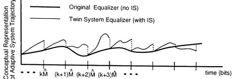
Figure 3: Conceptual representation of the adaptive system trajectory for the original, unbi-ased system (bold), and the equalizer in the twin system. The twin system equalizer adapts to the biased noise samples during a biasing cycle. At the beginning of a new biasing cycle, the equalizer in the twin system is then reset using tap values which would have resulted from unbiased noise samples.

properly (as our results will also show) in order to adapt to the biased signal

X*(k)

allowing

us to introduce more artificial errors into the system. Therefore, the TS estimator can

offer significant speed-up factors over the conventional

Me

estimator, as is also indicated in our empirical results. Fig. 3 illustrates the TS approach by showing a conceptual system trajectory. Each

if

bits is denoted here as a "biasing cycle". The bold curve in Fig. 3 represents the adaptive equalizer trajectory in the original, unbiased system. This is only

a conceptual plot since the equalizer trajectory is multidimensional. The plot is useful,

however, in understanding the basic idea behind the method. The thin curve denotes the trajectory of the twin system. In this system, biased noise samples are fed into the adaptive equalizer. An estimate of the BER is taken once each biasing cycle. The equalizer in the twin system is then "reset" to the trajectory which would have resulted had there been unbiased noise samples input (taken from the original system).

The variance of the instantaneous TS estimator is

O"~.

(k) =

f

O"~.

(k) fXc(k)(

a)

da

e,TS e,TSIXc(lc)

where the conditional variance O"~. (k) is given by

e,TSIXc(Jc)

(13)

(j2

==

_1

f

fX(k)(b) (wX(k)(b) - PeIXc(k)(k)) db

(14)

P:.TSIXc(It)(k) N* J{OX)Xc(k)}

P_eIXc(k)(k) is the probability of a detection error at time k conditioned on Xc (k), and

{X(k) : I(X*(k)h;;(k))

==

11

Xc(k)}

Importance Sampling Methodologies ... , Al-Qaq, Devetsikiotis, & Townsend

The variance of the TS estimator of

(12)

is given by (with N* in

(14)

set to unity)

10

(15)

where up. (kM)P. (1M) is the covariance of the estimates

Pe~Ts(kM)

and

Pe~Ts(lM),

k

=J

1,

e,TS e,TS

which are found using (11) with N* = 1. Our goal is to choose fX(kML) for ko

<

k

:s

K*

such that the first sum of (15) is minimized. The effect this will have on the second double summation is not clear, but our experimental results show large run time speed-up factors for a static linear channel, and a slowly varying, random linear channel. The choice of fX(k)

determines the magnitude of the estimator variance and is, therefore, crucial for the resulting

speed-up factor over conventional

Me.

3.2

Alternative IS Based on the Independence Assumption

Before we focus on finding an fX(k) that will minimize or nearly-minimize the estimator

variance, we present an alternative approach to the TS method. This alternative is based on a widely used assumption in the adaptive filtering literature, namely that the random data vector X( k) and the random vector he q (k) are statistically independent [9] . Under this

assumption, eq. (3) can be rewritten as

(16)

where

WX(k)(

a)

=

fX(k) (

a)/

fX(k)(

a)

This implies the following IS-based block simulation approach: Allow the trajectory of the

original adaptive system to evolve without biasing. For each block of

M

bits (i.e.,

M

x L

samples) make an IS-based decision by observing a biased output

X*(k)h;q(k),

where

X*(k)

is drawn independently from the X( k) that has already been used for the simulation and, therefore, independently from he q (k). The corresponding instantaneous IS estimator (called

here the instantaneous IA estimator) is given by

Pe~lA(k)

=

~* tI(X*(k,i)h~q(k,i))WX(k)(X*(k,i))

1=1

Similarly, the IA estimator equivalent to the TS estimator of

(12)

is given by

(17)

K·

Pe~lA

=

K*

~

k

L

I(X*(kM

L)h~(kM))wX(kML)(X*(kM

L))

(18)

ok=ko+1

Importance Sampling Methodologies ... , Al-Qaq, Devetsikiotis,

&

Townsend ₁₁

approach is that, as we will discuss in the sequel, an optimalbiasing setting is readily avail-able. In

gener~, ~owe~er,

.the IA estimator is a statistically biased estimator of P_e(k). The

amount ?f statistical bias IS dependent on how well the independence assumption describes

the specific system model at hand. Our empirical results indicate that most of the time

~h:

IA estimator yields results that are acceptably close to the TS

esti~ator.

In practice, It IS left to the experimenter to choose which one to use, based on the trade-off between

statistical bias and simplicity.

The preceding development of the IA method is based on the assumption that X(

k)

and he q (k) be statistically independent. The IA method, as it is actually implemented, only requires the weaker condition that the noise component N(k) of X(k) are statistically

independent of heq(k).

In the application section, we will compare this alternative IA estimator with the TS estimator and present empirical data on its statistical accuracy and relative statistical bias.

3.3

Optimal IS Biasing for TS and IA Estimat ors

As was stressed earlier, the choice of fX(k) determines the magnitude of the estimator variance

and the resulting speed-up factor over conventional Me. We restrict our attention to the

translation biasing scheme, which has demonstrated the best improvement in the past for

similar (although not time-varying or adaptive) models [6, 10, 7, 8]. In the translation scheme, we define the biased random vector as

X*(k)

=

X(k)

+

c(k).

We call

c(k)

the translation vector at the kth instant. The biased pdf is then simply fX(k)(X)

=

fX(le)(X

-c(

k)).

Our goal is to choose a translation vector c(k) at each decision instant k such that the conditional variance given by

(14),

and therefore the estimator variance in

(13)

(and the first summation in (15)) are minimized. For non-adaptive systems, and for the case corresponding to i.i.d. Gaussian inputs to a static, linear receiver filter, with impulse response h, it was implied in [6] and proved in [10] that the optimal translation is in the direction of the impulse response h, i.e., it is best to set c(k)

=

C( k)h. Thus, the optimal translation vector at instant

kis given by Copt (k)

=

Copt (k)heq( k) where Copt (k) is found by differentiating the estimator

variance expression with respect to

C(k)

and setting the result to zero. The optimal value

Copt under these conditions, was also found in [6].

In our case, the "input" vector X(

k)

is still Gaussian and uncorrelated, but in general, X(k) will have a covariance matrix, ~x(k). In order to apply IS to this X(k) we need to extend the results in [6, 10] appropriately. We do this in the Appendix, where we show that the optimal translation vector copt is then

(19)

and furthermore we obtain the optimal translation amount Copt (

k).

Another important point for the application of the above result to a time-varying(but still non-adaptive) system is that the optimal translation vector needs to be re-evaluated for ~very

Importance Sampling Methodologies ... ,

AI-Qaq,

Devetsikiotis,

&

Townsend

12

Finally, for our adaptive system model, the abovecopt(

k)

will no longer be optimal unless the equivalent system response

h;q(k)

is statistically independent of the input vector X*(

k)

at time k. The implications for our techniques are the following: All TS estimator is statis-tically unbiased, but the above Copt (

k)

is optimal only to the extent that the independence

assumption is true. For cases where that assumption is not true, no strictly optimal IS

translation setting is available right now. On the other hand, the IA estimator, although statistically biased, immediately admits this Copt (

k)

as optimal with no complications.

Our empirical observations indicate that either estimator can be used with very significant

speed-up factors over conventional

Me.

4

Applications and Experimental Results

4.1

Set- Up

In order to verify the effectiveness of applying the IS scheme to adaptive systems, several

simulation experiments were performed. The technique was applied to a system with a 6-tap LMS adaptive equalizer. The step size of the algorithm was found for each experiment by estimating the power of the signal at the input of the equalizer.

Two channels were considered, a static linear channel, and and a randomly time-varying

channel. The static channel had a normalized impulse response

v(l)

==

(a)l/~t!~L-lv2(1),

1

==

0, ... ,MIL - 1with a

<

1 a user-selected parameter.

The time-varying channel consisted of a uniformly distributed multiplicative factor fol-lowed by a static linear channel similar to the above:

s(1)

==

v(1)

*

a(l)r( 1)

where

r(l)

was uniformly distributed, centered at 1.0, with a total spread of 0.6, and

g(.)

the same as above. Our artificial random "fading" was made slow by holding the same value of

r(

1)

for the entire duration of a bit. Fig. 4 shows the impulse response of the static linear channel used and plots of the equivalent impulse response

g(

k,

t)

of the time-varying channel at three different time instants, t

==

18, 36, and 72. In both types of channels, a memory of two bits

(M

1

==

2) was considered.

Baseband binary signaling was used in the examples, with levels of

-A

and

+A

cor-responding to 0 and 1 data values respectively, with a signal level A

==

5. The Gaussian

noise was zero mean with variance u2

₌₌

_{0.5. The receiver filter was a one bit}

_(M

2

==

1)

matched filter. As stated earlier, the equalizer memory length was M

==

6. Throughout our

experiments we used L

==

9 samples per bit. The signal-to-noise ratio (SNR) for the example

systems was

SN R

~ 27dB. In each experiment, the adaptive equalizer was initialized to

zero, then trained for a short period of time (100 rv 200 bits).

In the twin system experiments, Pe~TS were obtained according to (12) for each channel

configuration. Decisions were spaced

M

bits (where

M

is the memory of the equivalent

system

_heq).

The noise vector

N(k)

was biased along the direction of the equivalent impulse

Importance Sampling MethodolotTies_{o- ... ,} Al-Qaq_,eveD t·1O ti

&,."

d

S1 0 1S, .Lownsen

₁₃

0.3r---,r---~--~----:---__r_--__r_--~--..,.__-___,

0.2 0.25

.,-~

~

'U

:",

t:

o c..

CI')

~

..

u

: 0.15 [

~ 0.1

>

Co-~

0.05

v(k)

g(!c.13)

g(k~6)

g(k.72)

•. . 6 . . . - • •

..._ .

''''\

\ \

\

\ .

,"

.

:.../'.

...•._...

~ : .

",

...

13 16

1-1-12

10 3

6

4

2

OL---.:.-~---..;...--~---.:.---~---'

_a

time(k)

Figure 4: Plot of the time-varying impulse response of the channel for four different values

Importance Sampling Methodologies ... , Al-Qaq, Devetsikioiis,

&

Townsend

System nd

Pe~TS

;2

A 95

%

Confidence Speed-up

P:

T S

Static 833 1.6X10-5 4.5xI0-1 1 (1.4 X10-5

, 3.8X10

2

a == 0.94 1.7X10-5 )

Static 1300 2.7X10-8 1.2X10-16 (2.4 X10-8_{, 1.5X10}5

a == 0.928 3.0X10-8₎

Static 1500 9.7X10-11 1.7X10-21 _(8.6X10-1 1_{, 3.4X10}7

a == 0.92 1.1X10-1°)

Time- 833 1.0X10-5 8.9X10-1 1 _(7.4X10-6_{, 10}2

Varying 1.3X10-5 )

a == 0.925

Time- 1500 2.7X10-9 _3.7x10-17 _(1.0X10-9_{, 1.82X10}4

Varying 4.4X10-9 )

a:== 0.9

14

Table 1: Simulation data and speed-up factors for static and time-varying systems with an adaptive equalizer. Importance sampling based on the twin system approach was used in the simulations.

simply diagonal. Estimates of Pe~IA using the independence assumption were obtained during

the same experiments. These estimates, as mentioned earlier, did not require the twin

equalizer to adapt. Random vectors

N*(k)

for this estimator were drawn independently of

the

N

(k ),

from the biased (translated) pdf.

4.2

Results

Tables 1 and 2 summarize our experimental observations. In calculating confidence coeffi-cients and speed-up factors we replaced the "true" BER (which was unknown) by the TS

estimate. Between 833 and 1500 decisions per run

(nd),

with 50 runs were made for each

system in order to obtain the sample variance, ;;'2.

Notice the exceptional speed-up factors over conventional

Me,

which become unique

when recalling that this is the first application of IS to the simulation of adaptive systems. It is also remarkable that these speed-up factors were obtained with a suboptimal biasing procedure Recall, however, that the TS estimators are theoretically statistically unbiased. Thus, the suboptimality of the IS parameter settings used here only affected the speedup-factor. The relative statistical bias of the IA estimator is minimal to modest and suggests that this estimator deserves more study.

The measured overhead of the twin system technique (twin system implementation, opti-mal translation calculations etc.) was modest, reducing the net speed-up by roughly a factor

of 2 (~ 40/72) for a 6-tap equalizer, and a factor of approximately 3.5 (~ 41/145) for a

Importance Sampling Methodologies ... , Al-Qaq, Devetsikiotis, & Townsend

System nd

P~IA

u2 ... ReI. Bias,I A 95%Confidence Speedup

P:IA

Static 833 5.6X10 6 8.9X10 12 _{0.65 (4.8 x 10-}6_{, 6X10}2

a == 0.94 6.4X10-6 )

Static 1300 7.3x10 9 3.1X10 17 0.73 (5.8x10-9_{, 1.4X10}5

a == 0.928 8.8X10-9)

Static 1500 1.3X10 11 1.1X10 22 0.87 (1.0X10-1 1_{, 6.0X10}7

a == 0.92 1.6X10-1 1)

Time- 833 3.0X10 6 1.5X10-1 1 _{0.7 (1.9X10-}6_{, 1.4X10}2

Varying 4.1X10-6₎

a == 0.925

Time- 1500 6.8x10 11 5.0X10-20 _{0.97 (6.0X10-}1 2

, 8.0X104

Varying 1.3X10-10)

a == 0.9

15

Table 2: Simulation data and speed-up factors for static and time-varying systems with an adaptive equalizer. Importance sampling based on the independence assumption approach was used in the simulations.

5

Conclusions

We have presented, for the first time, two IS methodologies for

Me

simulation of

commu-nication links characterized by time-varying channels and adaptive equalizers. In the TS method, biased noise samples are input to the adaptive equalizer, but the equalizer is only allowed to adapt to these samples for a time interval equal to the memory of the system. The TS method results in a statistically unbiased estimator, and circumvents the problems associated with system memory which increases with time in the simulation.

In addition to the TS technique, we also present a statistically biased, but simpler tech-nique for using IS with adaptive equalizers which is based on the independence assumption between the equalizer input and the equalizer taps (the "IA" technique).

Experimental results show run time speed-up factors of two to seven orders of magnitude for a static linear channel with memory, and of two to almost five orders of magnitude for a slowly varying, random linear channel with memory for both the IA and TS methods.

Acknowledgement

The authors would like to thank the anonymous reviewers for their helpful comments

and suggestions.

References

[1]

S. S. Haykin. Adaptive Filter Theory. Englewood Cliffs, New Jersey: Prentice-Hall,

1986.

Importance Sampling Methodologies ... , Al-Qaq, Devetsikiotis, & Townsend 16

[3] P. Balaban. Statistical Evaluation of the Error Rate of the Fiberguide Repeater Using Importance Sampling. Bell Sys. Tech. J., 55(6):745-766, Jul.-Aug. 1976.

[4]

K. S. Shanmugan and

P.

Balaban. A Modified Monte-Carlo Simulation Technique for the Evaluation of Error Rate in Digital Communication Systems. IEEE Trans. Commun., COM-28(11):1916-1924, Nov. 1980.

[5] M. C. Jeruchim. Techniques for Estimating the Bit Error Rate in the Simulation of Digital Communication Systems. IEEE J. Select. Areas Commun., SAC-2(1):153-170, Jan. 1984.

[6]

D. Lu and

K.

Yao. Improved Importance Sampling Technique for Efficient Simulation of Digital Communication Systems. IEEE J. Select. Areas Commun., 6(1), Jan. 1988.

[7] M. Devetsikiotis and J. K. Townsend. A Useful and General Technique for Improving the Efficiency of Monte Carlo Simulation of Digital Communication Systems. In Proc. of IEEE GLOBECOM '90, San Diego, CA, 1990.

[8] M. Devetsikiotis and

J.

K. Townsend. An Algorithmic Approach to the Optimization of Importance Sampling Parameters in Digital Communication System Simulation. To appear in the IEEE Trans. Commun.

[9]

N.

J. Bershad and L.

Z.

Qu. On the Probability Density Function of the LMS Adaptive Filter Weights. IEEE Trans. Acoustics, Speech, and Signal Processing, 37:43-56, Jan. 1989.

[10] R. J. Wolfe, M. C. Jeruchim, and P. M. Hahn. On Optimum and Suboptimum Bias-ing Procedures for Importance SamplBias-ing in Communication Simulation. IEEE Trans.

Commun., COM-38(5):639-647, May 1990.

Appendix

We present here an extension to the findings in [6] and [10]. Both the optimal transla-tion directransla-tion and the optimal translatransla-tion amount are found for the case of correlated, non-identically distributed Gaussian inputs to a linear system.

Specifically, suppose that the M-dimensional vector x is Gaussian distributed, with mean

m and covariance matrix ~x (note that in this Appendix vectors should be taken as column vectors). Let .Pe·(h,m,~x,c) be the IS estimator

P,,*(h,m,:Ex,c)

=

~'tho(hTxnwx(xi)

1=1

of the probability

Pe(h,

m,~x) ==

P{h

TX

>

To

I

h, m, ~x}

Importance Sampling Methodologies ... , Al-Qaq, Devetsikiotis,

&

Townsend ₁₇

Our goal is to find a translation vector c, such that the estimator variance is minimized. Under the given assumptions, the estimator variance is

u;s(h,

m,

:Ex,

c)

where

and

{

( X c)T~-l(X

c) }

B(x,c)

=

exp - - 2x

-Minimizing

o-Js(h,

m, :Ex,'c)

is equivalent to minimizing

V(h, m,

~x,

c)

=

E(Pe*2(h,

m, :Ex, c)),

with respect to c. It follows after some algebraic manipulation that

(

)

{

T

-1}

(To-hTm+hTc)

V

h,m,~x,c

=

exp

c

~x

c

Q

(hT~xh)1/2

Let

Co

=

h

Tc be the effective translation at the output, and

u

2

₌₌

hT~X_{h be the output}

signal variance.

Optimal direction: Let T be a non-singular linear transformation and

x'

==

Tx

m'

==

Tm

~~

==

Tbx T T

Then

V(h,

m,

bX,

c)

==

V(h',

m',

b~,

c')

when

h'

==

(T-1

)Th

and

c'

==

Tc.

Let

1

M denote

the identity matrix of dimension

M

x

M.

Choose

T

such that ~~

==

U~IM, for some

ui,

i.e.,

T

diagonalizes and normalizes

bx.

Such a transformation always exists because ~x is symmetric and positive definite.

,

21

V(h' ,~, '). . . . d

a1

th From [10] we know that, when ~x

==

U 1 M, ,m ,LJx,c IS mmimize ong e

direction

h',

i.e., c' == C~th'. It follows that for all c,

V(h,

m ,

~x,

c)

V(h',

m',

~~,

c')

>

V(h',

m',

~~,c'opt) V(h,

m,

~x,T-1

c'opt)

V(h,m,~x, C~tT-lh')

Therefore V(h, m,~x,c) is minimized forCopt

==

C~tT-lh' == C~tT-l(T-l

)Th

==

C~t/ui~xh,

since T~x

TT

==

uiI

M implies bX /

ur

==

T-

1

(T-

1

)T.

We conclude that V(h,m,~x,c) is

Copt-Importance Sampling Methodologies ... , Al-Qaq, Devetsilciotis, & Townsend 18

Optimal translation amount: When c == C~xh, it follows that cT~X1C=

C

O

/ O'

2, since

and

c~ ==

(h

Tc)2 ==

C2(hT~xh)2 ==

C 2

O'

4

Therefore, when c

==

C~xh, the estimator mean square value can be written as a function

of a scalar quantity Co:

,

(To -

hTm

+

Co)

V(h,m,Lx,c)

= V(h,m,LX,CO ) =exp(Co)Q u

which is the same mean square term minimized in [6]. Using similar manipulations (and the

common

Q(.)

approximation when its argument is greater than

4),

one finds