An Optimal Low Power Adaptive Filter Design For Noise Reduction

An Optimal Low Power Adaptive Filter Design For

Noise Reduction

Pallavi Sathawane#1_{, D.V.Prasanthi}#2

#1 PG scholar (VLSI) #2 Assistant Professor

Department of electronics and communication engineering Gokaraju Rangaraju Institute of engineering & technology,JNTUH

Abstract— Here this paper present an architectural approach to

design an adaptive filter with low power consumption. Basically, an adaptive filter comprises of a variable filter and a filter coefficient updating algorithm. The variable filter is an FIR filter due to its stability, which has larger amplitude variations in input data and filter coefficients. As filtering part is the major contributor of power in an adaptive system, cancellation of multiplication will cause a significant reduction in power. To perform the adaptation process, that is convergence of output computed by the variable low power FIR filter to a desirable output least mean squares (LMS) and recursive least squares (RLS) algorithm is available. As one of the important applications of adaptive filtering, noise cancellation in communication system is performed on a signal with injected noise. The low power architecture for adaptive filter system which consists of a reconfigurable and low power FIR filter for filtering process and LMS algorithm for the adaptation process is designed .The low power adaptive filter architecture is verilog coded and simulated on Modelsim to check desired functionality .Then filter design is synthesized on Xilinx ISE suit for generating power report. Experimental results show significant reduction in power.

Keywords

—

As the scale of integration keeps growing, more and more sophisticated signal processing systems are being implemented on a VLSI chip. These signal processing applications not only demand great computation capacity but also consume considerable amount of energy.

Real-world signals which are analog in nature need to be processed so that the information contained in them can be displayed, analyzed or converted to other useful form, which is performed by a digital signal processing (DSP) system. Digital signal processing has been executing a major role in the current technical advancements such as noise cancellation, echo cancellation, voice prediction etc. So, for obtaining quick and acceptable solutions for these problems adaptive filtering techniques must be implemented other than standard DSP techniques. In general, filtering is one of the widely used operations in digital signal processing (DSP). A filter is a signal selection system that is used to extract desired

signal from a noisy signal which consists of disturbances, whereas adaptive filter is particularly useful whenever the statistics of the input signals to the filter are unknown or time varying and the design requirements for fixed filters cannot easily be specified. The basic operation of adaptive filter involves two processes: a filtering process and an adaptation process. The filtering process is usually fir filtering due to stability measures. The adaptation process uses an adaptation algorithm to update the filter coefficients according to the working environment. As filters are one of the major determinants of performance and power consumption of the whole system, there is an increased concern for designing low power filter structures. Digital filtering is an integral part of modern approaches to signal and image processing. This application is used in many domains (automation, telecommunications, biomedicine, etc.) As the paper aims to design a low power FIR adaptive filter, a summary of earlier efforts on reducing power consumption of FIR filter is discussed below.

Several works on lowering power consumptions of FIR filters have been proposed earlier. Some previous works have tried to optimize the filter coefficient while maintaining fixed filter order. In those approaches, filter structures are simplified to add and shift operations and the power reduction is achieved by minimizing number of additions. However, one of the major drawbacks of such approaches is that the coefficient cannot be changed, once the filter order is fixed. There for those techniques are not applicable to the FIR filters with programmable coefficients. An improved algorithm is presented for the discrete optimization of FIR digital filter coefficients which are represented by a canonic signed-digit (CSD) code, i.e., numbers representable as sums or differences of powers-of-two. The proposed search algorithm allocates an extra nonzero digit in the CSD code to the larger coefficients to compensate for the very non uniform nature of the CSD coefficient distribution. This results in a small increase in the filter complexity[14]. For the design of low power FIR filters, approximate signal processing techniques [18] has also been used. In energy scalable system design [17], it is shown that sorting the data samples and coefficients before convolution operation has some energy quality characteristics. In this approach, for desirable energy quality behaviour of FIR filter, MAC cycles that contribute

significantly to the filter output is accumulated first by sorting. However, the overhead due to the real-time sorting of data samples is too large.

I. ARCHITECTURE OF LOW POWER ADAPTIVE FILTER

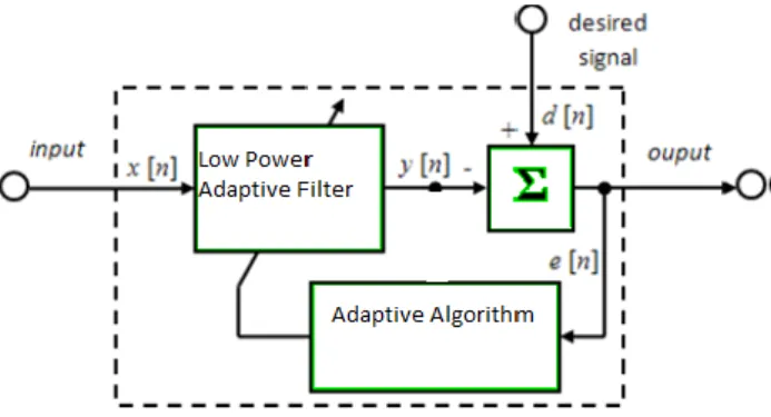
An adaptive filter is a digital filter that has self-adjusting characteristics. Adaptive filters, on the other hand, have the ability to adjust their impulse response to filter out the correlated signal in the input. They require little or no a priori knowledge of the signal and noise characteristics. (they require a signal (desired response) that is correlated in some sense to the signal to be estimated). Moreover adaptive filters have the capability of adaptively tracking the signal under non-stationary conditions. The general block diagram of an adaptive filter is given in Figure1. Adaptive filters are composed of three basic modules such as filtering structure, performance criterion and adaptive algorithm. The filtering structure determines the output of the filter from given input samples. FIR is preferred over the IIR for filtering due to stability measures. Then, the performance criterion is chosen according to the application and it is used to derive the adaptive algorithm. The three generally used performance criteria are mean squared error, least squares and weighted least squares. Finally, the adaptive algorithm is used to update the filter coefficient based on the performance criterion to improve the performance.

Fig 1 :General Block Diagram of Adaptive Filter

The three generally used performance criteria are mean squared error, least squares and weighted least squares. Finally, the adaptive algorithm is used to update the filter coefficient based on the performance criterion to improve the performance. The low power adaptive filter as shown in figure.2 consists of a low power and reconfigurable FIR filter for filtering process and LMS algorithm for adaptation process. Here the performance criterion based on which LMS algorithm update filter coefficients is mean square error value.

Fig 2:Block Diagram of Low Power Adaptive filter

II. RECONFIGURABLE FIR FILTER ARCHITECTURE

Finite impulse response (FIR) filters are digital filters that have a finite impulse response. FIR filters operate only on current and past input values and are the simplest filters to design. FIR filters also are known as non recursive filters. This can be stated mathematically as

where n1 and n2 lies between –∞ and ∞, h(n) denotes the

impulse response of the digital filter, n is the discrete time index, and n1 and n2 are constants. A difference equation is the

discrete time equivalent of a continuous time differential equation. The FIR filter we have been considering has two important properties

– Linearity – Time invariance

The general difference equation for a FIR digital filter is

where y(n) is the filter output at discrete time instance n, bk is the kth feed forward tap, or filter coefficient,

and x(n-k) is the filter input delayed by k samples. The Σ denotes summation from k = 0 to k = n-1 where n is the number of feed forward taps in the FIR filter. FIR filters are the simplest filters to design. If a single impulse is present at the input of an FIR filter and all subsequent inputs are zero, the output of an FIR filter becomes zero after a finite time. Therefore, FIR filters are finite. The time required for the filter output to reach zero equals the number of filter coefficients. Equation describes the behaviour of the filter only in terms of current and past inputs. So FIR filter are also known as non recursive filters.

Power consumption of FIR filter is directly proportional to the amount of computation. To reduce the power consumption, the proposed FIR filter structure cancels multiplication. The architecture is reconfigurable because it changes the filter order dynamically by considering the amplitude of data samples and filter coefficients. The performance of the filter is still maintained by making the

product of data sample and the filter coefficient as small as the quantization error.

Fig 3: Direct Form Architecture of Conventional FIR Filter

Fig.4 shows the architecture of reconfigurable FIR filter. It consists of three main sections. Amplitude Detector (AD), Multiplier Control Signal Decision window (MCSD) and a control signal generator. The architecture reduces the power consumption by cancelling multiplication. More specifically, the dynamic power is reduced because it is directly proportional to switching activity.

Fig 4: Architecture of Reconfigurable FIR Filter

As specified earlier, the proposed reconfigurable architecture dynamically changes the filter order when multipliers get turned off based on the filter coefficient and data sample amplitudes. The criterion for cancelling the multiplications is that the amplitude of both data sample and filter coefficient is less that predetermined threshold value or

not. If the amplitude of the incoming data sample is smaller than the threshold (𝑥𝑡ℎ_{), the output of AD (ad_out) becomes}

―1‖. One problem that occurs while using this logic is that, if the amplitude of the input data samples changes abruptly for every cycle, then the multipliers will be turned off and on continuously. This in turn increases the switching activity and thus the dynamic power increases. To solve this switching problem Multiplier Control Signal Decision window (MCSD) is used which is explained in the following section. For the low power adaptive filter, AD is required for each filter coefficient as the amplitude of the coefficient is varying. The amplitude detector for each filter co-efficient compares the amplitude of the coefficient with a predetermined threshold value (𝑐𝑡ℎ_{) and if it is smaller, then the output (ad_coeff)}

becomes ―1‖. Multiplier Control Signal Decision window (MCSD) is used to reduce the frequency of switching activity. There is a control signal generator within the MCSD window which reduces the switching problem. The control signal generator consists of an internal counter which counts the number of input samples for which the condition [𝑛]<𝑥𝑡ℎ _is

satisfied. That is, the counter starts counting up whenever the output of the amplitude detector (ad_out) is set to ―1‖. When the count reaches certain value (say m), the output of the control signal generator (ctrl) becomes ―1‖, where m is the size of MCSD .So, a ―1‖ value on ctrl is an indication that 𝑚 consecutive small inputs are monitored and multipliers are ready to turn off. The signal ctrl also controls an additional signal 𝑖𝑛𝑐𝑡−𝑛. This signal accompanies with the input data all the way in the following flip flops to indicate that [𝑛]<𝑥𝑡ℎ_{, and}

the multiplications can be cancelled if the corresponding filter coefficient amplitude is smaller than 𝑐𝑡ℎ. In figure 8.2 an additional delay element is added before the first tap to synchronize 𝑖𝑛𝑐𝑡−𝑛 and 𝑥∗(𝑛). The procedure of turning off the multiplier after getting the filter coefficient and data sample smaller than the corresponding threshold is as follows. When the amplitude of the input data sample and filter coefficient is smaller than the thresholds, the signal 𝜑𝑛 is set to ―1‖. Whenever the signal 𝜑𝑛 is set to logic ―1‖, the multiplier will be turned off by a simple logic circuit and the output in turn forced to zero. An important thing to consider while designing the reconfigurable filter section is the values for the threshold 𝑥𝑡ℎ _{and 𝑐}𝑡ℎ _{, which has a significant impact}

on the filter performance and power consumption. If the threshold values are very large, it can give rise to large power savings at the cost of filter performance. On the other hand if the threshold values are small, then the power savings become trivial. Similarly the values of 𝑚, indicating the size of MCSD also have significant impact on the power savings. So, if 𝑚 becomes larger, then the number of input samples that makes multipliers turned off decreases. Then the power reduction becomes smaller and filter performance degradation becomes lower as well.

III. ADAPTATIONALGORITHM

The basic configuration of an adaptive filter, operating in the discrete-time domain n, is illustrated in Figure 1. In such a scheme, the input signal is denoted by x(n), the reference

signal d(n) represents the desired output signal (that usually includes some noise component), y(n) is the output of the adaptive filter, and the error signal is defined as e(n) = d(n) −

y(n). The error signal is used by the adaptation algorithm to

update the adaptive filter coefficient vector w(n) according to some performance criterion. In general, the whole adaptation process aims at minimizing some metric of the error signal, forcing the adaptive filter output signal to approximate the reference signal in a statistical sense. There are several adaptation algorithms with different performance criterion. Due to its low complexity and proven robustness, Least Mean Square (LMS) algorithm is used here.

The LMS algorithm is an iterative formulation which solves, in the limit, the Wiener-Hopf equations recursively using a stochastic approximation to the method of steepest descent.

Wiener-Hopf solution for optimum filter weights shown in below equation

LMS algorithm is a noisy approximation of steepest descent algorithm. It is a gradient-type algorithm that updates the coefficient vector by taking a step in the direction of the negative gradient of the objective function.

where μ, is the step size controlling the stability, convergence speed and misadjustment. To find an estimate of the gradient, the LMS algorithm uses an objective function considered as the instantaneous estimate of the mean square error, i.e., Jw = 𝑒2_{(𝑛) resulting in the gradient estimate 𝜕𝐽𝐰/}

𝜕𝑤(n) = −2𝑒(𝑛) 𝑥( 𝑛) . LMS Algorithm: For each n { y(n) = wᵀ (n)x(n) e(n) = d(n) – y(n) w(n+1) = w(n) + 2μ e(n)x(n) }

As discussed earlier, the LMS algorithm update the filter coefficient for tracking the desired filter output using the error signal (e(n)). In the mathematical model, y(n) is the computed filter output, wᵀ (n) is the filter coefficients in transposed form, x(n) is the filter input samples, e(n) is the error signal which used for updating the filter coefficients and

μ is the step size or the learning factor. Figure.5 shows the

general direct form LMS adaptive filter structure for updating filter tap weights. The filter tap weights are updated using the equation w(n+1) = w(n) + μe(n)x(n), ie., the new filter tap

weights are generated from the current tap weight based on the step size, error signal.

Fig 5: Direct form LMS adaptive filter structure (conventional)

IV. ADAPTIVE NOISE CANCELLATION

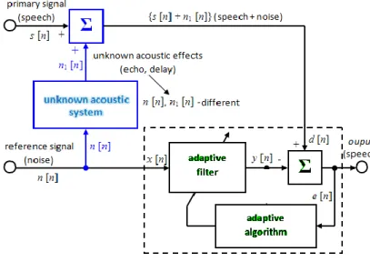
Figure 6. is a principled scheme of the adaptive system in which simulations of adaptive algorithms LMS is conducted. Principles of this scheme are implemented in Matlab using the source command. so the libraries for adaptive filtering which Matlab includes is not used, but its own source code based on knowledge of the mathematical interpretation of adaptive algorithms is created.

Fig 6: Adaptive Noise Cancellation

In order to use the adaptive system diagram in Figure 6 in practice, an additional (reference) microphone must be appropriately placed into some part of the noisy environment, so that we were able to record the noise directly.

In practice, the choice of a suitable location of the reference microphone, is a serious problem (e.g. hands free in cars), because the microphone has to record only the interference signal (noise), without the useful signal (speech) and the effort on the minimum difference with the reference noise n[n] and the primary microphone n1[n] is additional. Now we came to the fact that the noise at the primary and reference microphone is not the same. This is caused by a number of unidentified acoustic phenomena such as echoes, various distortions in the sound barriers, and last but not least it is the audio delay caused by different pathways (times) of the dissemination of the audio signal from the signal source to the microphone (the formation of the echo as well).

V. SIMULATION RESULTS

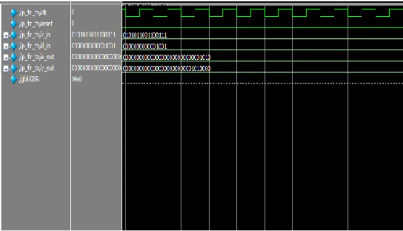
The low power adaptive filter is Verilog coded and simulated on ModelSim to check the desired functionality. The filter specifications are 16 bit data samples, 16 bit filter coefficients. For comparison we have verilog coded the conventional filter structures. Figure 7 shows the ModelSim snapshots of conventional FIR filter. The simulation results of conventional and low power adaptive filter is shown in Figure.8 and Figure.9. The filter structured in Verilog is synthesized on Xilinx ISE. The Xpower analysis on Xilinx provides the power report.

Fig 7: Simulation result of conventional FIR filter

Fig 8: Simulation result of conventional adaptive filter

Fig 9: Simulation result of low power adaptive filter

Fig 10: Power report of conventional adaptive filter

Fig 11: Power report of low power adaptive filter

VI. CONCLUSIONS

In this paper, low power architecture for adaptive filter is proposed. The low power adaptive filter consists of a reconfigurable low power FIR filter and the LMS algorithm. The LMS algorithm is used to update weights of reconfigurable filter with low complexity. The experimental results showed significant reduction in power. The application of low power adaptive filter to noise cancellation is demonstrated using a signal with injected noise. The proposed

low power adaptive filtering system can also be used for other applications such as system identification, echo cancellation etc.

.

FUTURE WORK

The low power adaptive filter can be implemented using vedic multiplier or by using neural network concept. By using vedic multiplier or neural network concept one can compare power report.

REFERENCES

[1] Benard Widrow ,S.D. Stearns, ―Adaptive Signal Processing‖ ,2nd _Edition

,ISBN 978-81-317-0532-2 ,2009.

[2] Li Tan , Jean Jiang, ―Digital Signal Processing Fundamentals and Application‖ , 2nd _{Edition ,ISBN 978-0-12-415893-1,2013.}

[3] Antoniou ,A.," Digital Filter",3rd _{Edition, Tata Mc. Graw Publications,}

2001

[4] Parhi K K., "A Systematic Approach For Design Of Digit-Serial Signal Processing Architectures",Circuits and Systems,1991.

[5] Saeid Mehrkanoon, Mahmoud Moghavvemi , ―Real time ocular and facial muscle artifacts removal from EEG Signals using LMS Adaptive Algorithm‖, International Conference on Intelligence and Advanced System,2007.IEEE [6] NJ Bershad, JCM Bermudez, ―An Affine Combination of Two LMS Adaptive Filter Transient Mean-Squre Analysis‖ Signal Processing, IEEE Transactions, May 2008.

[7] K. R. Borisagar, G. R. kulkarni ―Simulation and Comparative Analysis of LMS and RLS Algorithms Using Real Time Speech Input Signal‖ GJRE, 2010.

[8] Seok-Jae Lee, Ji-Woong Choi, Seon Wook Kim and Jongsun Park.(2011), ―A Reconfigurable FIR Filter Architecture to Trade Off Filter Performance for Dynamic Power Consumption‖, IEEE Trans. Very Large Scale Integr. (VLSI) Syst., vol. 19, no. 12, pp.

[9] R. Mahesh and A. P. Vinod .(2010), ―New reconfigurable architectures for implementing filters with low complexity‖, IEEE Trans. Comput.-Aided Des. Integr. Circuits Syst., vol. 29, no. 2, pp. 275–288

[10] R.Mahesh and A. P. Vinod.(2008), ―A new common subexpression elimination algorithm for realizing low complexity higher order digital filters‖, IEEE Trans. Comput.-Aided Design Integr. Circuits Syst., vol. 227, no. 2, pp. 217–219.

[11] Georgios Karakonstantis and Kaushik Roy (2007), ―An optimal algorithm for low power multiplier less FIR filter design using chebychev criterion‖, IEEE ICASSP., pp. II-49 – II-52

[12] Vaseghy, S. V. Advanced Digital Signal Processing and Noise Reduction, Second Edition, Chichester Wiley, ISBN 0-470-84162-1, 2000. [14] H. Samueli, ―An improved search algorithm for the design of booth's multiplierless FIR filter with powers-of-two coefficients,‖ IEEE Trans. CircuitsSyst., vol. 36, no. 7, pp. 1044–1047, Jul. 1989.

[15] R. I. Hartley, ―Subexpression sharing in filters using canonical signed digitbooth's multipliers,‖ IEEE Trans. Circuits Syst. II, Analog Digit. Signal Process., vol. 43, no. 10, pp. 677–688, Oct. 1996.

[16] O. Gustafsson, ―A difference based adder graph heuristic for multiple constant multiplication problems,‖ in Proc. IEEE Int. Symp. CircuitsSyst., 2007, pp. 1097–1100.

[17] A. Sinha, A. Wang, and A. P. Chandrakasan.(2002), ―Energy scalable system design‖, IEEE Trans. Very Large Scale Integr. Syst., vol. 10, no. 2, pp.135–145.

[18]. S. H. Nawab, A. V. Oppenheim, A. P. Chandrakasan, J. M. Winograd, and J. T. Ludwig (1997), ―Approximate signal processing‖, J. VLSI Signal