Self-healing of
composite material
with an intermediate
supramolecular
layer
Bachelor assignment for Advanced Technology
2
Summary
Around the start of the 21st century a new field of study emerged who concerns self-healing material. Self-healing material are a class of materials that have structurally incorporated ability to heal damage caused by mechanical use over time. In this research the self-healing supramolecular material SP1 is investigated.
SP1 maintains self-healing ability when acting as adhesive intermediate layer between two plies of composite material. Composite material is a class of materials which have lots of different applications and is used for many purposes.
In the first part of the research a production method is designed to make samples of composite material containing an intermediate supramolecular layer with uniform thickness. In the second part of the research a test method for a Double Cantilever Beam (DCB) test is designed in which the samples from the first part can be tested on its fracture toughness, which is a measure of the ability of a material containing a crack to resist fracture. Determining the fracture toughness after the material has supposed to heal itself can say something about the self-healing ability. In the third part of the research DCB tests are performed for several different composite samples containing an intermediate supramolecular layer which varied in thickness to find out the effect of this thickness on the fracture toughness.
4
Table of Contents
Summary ...2
Introduction ...5
Self-healing material ...5
Composite material ...5
Goal ...6
Theoretical Background ...7
Supramolecular material ...7
Fracture toughness determination ... 10
LabVIEW program ... 16
Execution ... 17
Composite Sample Production ... 17
Supramolecular intermediate layer production ... 19
Production of sample with intermediate supramolecular layer... 20
Double Cantilever Beam test ... 25
Preparation of Sample ... 25
Test method I ... 27
Test method II ... 29
Results ... 33
Angle measurement validation ... 33
Influence of the thickness ... 35
Conclusion and Recommendations ... 39
Conclusions ... 39
Recommendations ... 40
5
CHAPTER 1:
Introduction
In this chapter an introduction to the topics concerned in this bachelor assignment is given. There will be shortly explain how self-healing materials emerged and what composite materials are. In the last part of this chapter the goal of this bachelor assignment is declared.
Self-healing Material
Material nowadays have to meet high requirements. Especially in for example aerospace materials have to withstand high forces and need to have long durability. There is a lot of competition between airlines so aircrafts have to be built as cost-efficient as possible and have low maintenance costs. Maintenance can be reduced if materials do not need to be repaired but can heal themselves. A new emerging field of interest is the research and development of self-healing material. The last decade this research field started and in 2007 the first international conference on self-healing material was held in Noordwijk. Scientists got their inspiration for the creation of self-healing material from biological systems. Think about having a wound in your arm. Your body have the ability to transport the right substances to repair the wound to the right place. Eventually a crust will appear and then after some time your arm will looks like new. It can easily be understand that if something is also applicable in an artificial material it is very beneficial.
Composite Material
Composite material is a type of material which is widely used and have several different applications. A reason why composite materials are used so commonly is that a composite material is a material made out of 2 or more different components which combined together form a structure that is better than the sum of the individual components. Composite material have been used since the time of Ancient Egypt. In an old tomb paintings were found, on which bricks were produced out of a composite of mud and straw. The first plastic composite was discovered is the United States when someone accidentally spilled bakelite on his shirt. He eventually did not removed the stain so he could continue his work but when tried to remove the stain when he was finished with his work the stain was all hard and impossible to remove. This knowledge was the kickoff to a series of experiments which is nowadays still a very promising area of research.
All that research lead to the discovery of lots of composite materials which have applications in all kind of different fields like for example architecture, bridge construction, aerospace and automotive industry. The most well-known artificial composite material is concrete. Concrete is composed mainly of water, aggregate and cement. The aggregate in the concrete is held by a so called matrix of cement. A matrix is an important feature in a composite material and serves like a framework to support another component of the composite material. In fiber reinforced composite material, which is of great interest for this research, the matrix keeps the fibers together and takes care of the shear stress and the fibers on their side transfer the normal force responsible for stretching the material.
6
Goal
The goal of this bachelor assignment is to research the possibilities of a certain so called supramolecular material which promises to maintain self-healing capability when acting as an adhesive intermediate layer in a composite material. The capability of self-healing of a material can be determined by determining the interlaminar fracture toughness at this intermediate layer of a sample of composite material before it is damaged and after it have been damaged and have undergone a self-healing cycle. The fracture toughness is the property which describes the ability of a material containing a crack to resist fracture. By comparing the value found before the material is damaged with the value found after it was damaged and have undergone a self-healing cycle you can state if the material have self-healing capability. If those values are the same or only differ a few percent it is proven that the material indeed maintains self-healing capability. Previous research have been done into the supramolecular material SP1 which was an intermediate layer in between two plies of fiber reinforced composite material with a conventional thermoplastic matrix [1]. Self-healing ability was proven, but lots of aspects of the research were unreliable. The measurement method used for determining the fracture toughness was unreliable for most of the tests and the amount of measurements was low. The production of samples with an intermediate supramolecular layer was also done unreliable and an uniform thickness of the intermediate layer in the samples was not achieved as well as the effect of this thickness on the fracture toughness was not clear.
Goals of this bachelor assignment are therefor:
- Design a production method for samples with an intermediate supramolecular layer so that a uniform thickness is achieved
- Design a test method from which the measurement data is reliable.
7
CHAPTER 2:
Theoretical Background
This chapter provides a theoretical background to the process and calculations which are of importance to the subject of this bachelor assignment report. In the first paragraph the SP1 material that promises to have self-healing ability is introduced and there will be explained how in theory the self-healing process of this material works. In the second paragraph there will be explained how the possible self-healing ability of this material can be proven. In the last paragraph there will be shortly told how the software works which is used during execution of tests.
Supramolecular Material
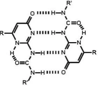
The material that will be used as an adhesive intermediate layer in the fiber reinforced composite material to provide self-healing capacity is a so called supramolecular polymer. A supramolecular polymer is a polymer whose monomer repeat units are held together by non-covalent bonds. In the supramolecular polymer used in this research, named SP1, after the company SupraPolix which produces it, those bonds are hydrogen-bonds. The monomer repeat units of SP1 have special endgroups named ureidopyrimidinone (UPy) groups which are capable of having four H-bonds (see
Figure 2.1). The reversibility of the H-bonds provided by the UPy groups makes the mechanical properties of SP1 strongly temperature dependent. At room temperature SP1 have a high viscosity and shows polymer-like viscoelastic behavior in bulk and solution. At elevated temperatures the H-bonds will break and SP1 will have a low viscosity and shows like properties. Due to the liquid-like properties of SP1, when a delaminated composite containing an intermediate SP1 layer get heated under low pressure a viscous flow of SP1 can fill that delamination and so the material can heal itself. The material so is not self-healing in a way that it does not need any (human) intervention to heal itself, an application of pressure and a supply of heat is needed, but actively repairing is not needed.
Figure 2.1: Chemical structure of quadruple hydrogen-bonded ureidopyrimidinone end groups. R and R’ represents an atom or a chain of atoms [2]
[image:8.595.213.382.478.626.2]frequency-8 dependent viscosity function determined during forced harmonic oscillation of shear stress. The main parts of this rheometer consists of 2 plates which are parallel to each other, one being stationary, the other able to rotate. A casing was put around this plates to control the temperature during testing. A sample of SP1 was placed on the bottom plate of the two parallel plate and the temperature was elevated until this sample is liquid. By reducing the gap between the plates and measuring the force at a certain angular frequency for the rotating plate, the viscosity of the sample at the given temperature was determined. The results are depicted in the two graphs Graph 2.1 and Graph 2.2. The two graphs clearly shows that the viscosity decreases as a function of temperature. Based on those results a temperature of between 100 °C and 140 °C will be used at production of the supramolecular intermediate layer, production of samples with supramolecular intermediate layer and healing process. A temperature higher than 140 °C is not used because at temperature near 150 °C the SP1 material will decompose and so losing its self-healing capacity for ever. [13,14]
9 Graph 2.2: Plot of complex viscosity vs angular frequency
10
Fracture toughness determination
To say something about the self-healing properties of SP1 when acting as an intermediate layer in a composite material the interlaminar fracture toughness at this layer of this composite material have to be determined. As was stated in the Introduction, the fracture toughness is the property which describes the ability of a material containing a crack to resist fracture. The fracture toughness is denoted by GIc and its unit is J/m2 and so is a measure of the energy required to grow a crack. The
[image:11.595.112.491.196.330.2]fracture toughness will be determined by testing samples of the composite material with a Double Cantilever Beam (DCB) (for production of samples, see Execution).
Figure 2.2: Sample of a DCB test. The hinges on the left end are the place where the sample will be clamped [3]
A Double Cantilever Beam test is the most common method of determining fracture toughness of composite material. In the test a sample of the tested material, which is in the form of a beam, is clamped at one end of the sample at both sides. (see Figure 2.2). The sample have to be pre-cracked to be able to determine the fracture toughness. This means that at the clamped end an initial delamination have to be present. This can be achieved by inserting a thin plastic film at this end in between consecutive layers of the material during production. The point where this layer is placed is the weakest spot in the sample so by preloading the sample at this place in a controlled manner a crack can be created.
[image:11.595.77.517.509.710.2]11 With a DCB test the mode I fracture toughness can be determined. Mode I, also known as opening mode, refers to the way a crack will propagate if a tensile stress normal to the plane of the crack will be applied. There are two other modes: the sliding mode (mode II) and the tearing mode (mode III). A mode II fracture will occur if a shear stress is acting parallel to the plane of the crack and perpendicular to the crack front. A mode III fracture will occur if a shear stress is acting parallel to the plane of the crack and parallel to the crack front. The three modes are depicted in Figure 2.3. So a mode I fracture will be created and therefor a force at the clamped end where the initial crack is will be applied. The crack propagation will continue, as long as a large enough force is applied, until the sample is divided into 2 plies. The test set-up will monitor this force (P), the displacement (δ) and the crack length (x) or angle of rotation (α) as shown in Figure 2.4. The exact way how the system monitors those values is elaboration in Execution. Parameter a is the curvature length but will not be monitored in the test set-up. Parameter B is equal to the width of the sample and parameter 2h
[image:12.595.91.504.265.471.2]equals the thickness of the sample.
Figure 2.4: Partially delaminated sample with representation of parameters [5]
From the measured values the fracture toughness can be calculated. Two separate methods will be used to calculate the fracture toughness, depending on wetter a sample containing an intermediate supramolecular layer is tested or one without an intermediate layer for which method is used. The first method is used for calculating the fracture toughness for a sample without an intermediate supramolecular layer. In this analysis the both arms of the DCB sample are considered to be fixed at the crack tip position. With the use of the linear beam theory a relation for the displacement δ of one single arm of a sample can be given by:
𝛿 2
=
𝑃𝑎3
3𝐸𝐼𝑥
(1)
In this equation is Ix the moment of inertia of a beam and given by Ix = Bh3/12 and E is the modulus of elasticity of the sample. When this relation for the moment of inertia of a beam is substituted in equation 1 a relation for the total displacement of the sample at the load line is given:
12 By making use of the linear elastic fracture mechanics the delamination energy, which is a measure for the fracture toughness, can be calculated. The fracture mechanics was developed during World War I by A. A. Griffith to explain the failure of brittle materials [6]. This theory was modified by G. R. Irwin et al. [7] and with those findings a relation for the fracture energy GIc is found when the crack at constant displacement δ grows with ∂a:
𝐺
𝐼𝑐=
2𝐵𝑃2∙
𝜕𝐶𝜕𝑎(3)
In this equation C is the compliance and is given by C = δ/P. This compliance can be written as:
𝐶 =
𝐸𝐵ℎ8𝑎33(4)
Differentiating C with respect to a and substituting this result in equation 3 gives:
𝐺
𝐼𝑐=
12𝑃2𝑎2𝐸𝐵2ℎ3
(5)
By making use of equation 2 this relation can be rewritten to an expression where E is a function of the other variables:
𝐸 =
8𝑃𝑎3𝛿𝐵ℎ3
(6)
Substituting this result from equation 6 into equation 5 the relation for the fracture energy becomes:
𝐺
𝐼𝑐=
3𝑃𝛿2𝐵𝑎
(7)
Equation 6 is the most common form for the fracture energy but some correction factors are taken into account for certain test conditions. In most standards three corrections are mentioned. The first one is a correction for a possible cross-section at the crack tip. The second is a correction for large displacements effects of the beam during test, which is effectively a shortening of the moment arm. And the last is a correction for the hinges mounted on the test sample, which adds extra stiffness to the sample. The derivation of the effects of the corrections is not elaborated in this report but the result to the relation for the fracture energy is:
𝐺
𝐼𝑐=
3𝑃𝛿2𝐵(𝑥+|∆|)
(8)
13 The second method of determining the fracture toughness from the measured values of a DCB test is for a sample with an intermediate supramolecular layer. This method makes use of the J-integral which is a way which was developed to determine the fracture toughness if there is sufficient crack-tip deformation that it no longer obeys the linear-elastic deformation. This was individually developed by both J. R. Rice and G. P. Cherepanov in the mid-1960s [4]. The mathematical definition they come up with for the J-integral is:
𝐽 = ∫ (𝑤 𝑑𝑦 − 𝑇
Γ 𝑖 𝜕𝑢𝜕𝑥𝑖𝑑𝑠)
with
𝑤 = ∫ 𝜎
0𝜀𝑖𝑗 𝑖𝑗𝑑𝜀
𝑖𝑗(9)
[image:14.595.77.526.334.455.2]In this equation Γ is an arbitrary path clockwise around the apex of the crack, w is the density of the strain energy, Ti are the components of the vectors of traction, ui are the components of the displacement vectors, ds is an incremental length along the path Γ and σij and εij are the stress and strain tensors. Unless there is not the situation during the DCB test that the sample no longer obeys the linear-elastic deformation, but during tests with samples with an intermediate supramolecular layer it is very difficult to measure the crack length x with the test set-up (test method I) which is elaborated in Execution. The J-integral approach reduces to the Griffith theory for linear-elastic behavior so this is approach is still usable for analysis the DCB test results.
Figure 2.5: J-integral approach on a DCB test sample by J. and C. Paris [8]
Anthony J. and Paul C. Paris elaborated on this approach [8]. In their analysis they also took a double cantilever beam sample of uniform rectangular cross section as shown in Figure 2.5. They took the contour of integration around the outer boundary of the sample. As a consequence, the contributions to this integral are zero everywhere except at the load points and there only through the traction term as long as the load points and crack tip are located remotely, more than h from the ends and each other. They let the traction there be constant, σ, over an increment, dx, so that:
𝑃 = 𝜎 𝑑𝑥
or
𝑇
𝑖= 𝜎 =
𝑑𝑥𝑃= 𝑐𝑜𝑛𝑠𝑡𝑎𝑛𝑡
(10)
Note that ds is dx or minus dx on the bottom or top contour respectively. Substituting this in equation 9 and evaluating this leads to:
𝐽 = 𝑃(
𝜕𝑢𝑦𝜕𝑥
|
𝑏𝑜𝑡𝑡𝑜𝑚−
𝜕𝑢𝑦𝜕𝑥
|
𝑡𝑜𝑝)
(11)
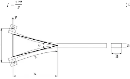
Or in the final form J. and C. Paris came up with:
14
In this equation θ is the relative rotation of the arms at the two load points as is also shown in Figure
2.6. But during the DCB tests in the used test set-up the load point and the crack tip are not more than h separated from each other so the dimension of the beam have to be taken into account. S.G. Ivanov [1] elaborated on this and came up with:
[image:15.595.83.510.138.397.2]𝐽 =
2𝑃𝜃𝐵(13)
Figure 2.6: Partially delaminated sample with representation of angle θ [5]
Figure 2.7: Geometric representation of relation between angle θ and α
The variable θ can be expressed as a function of the measured values α and δ. For symmetry reasons
the situation as depicted in Figure 2.7 holds. For geometric reason the top angle of Δklm equals α
[image:15.595.140.450.427.647.2]15
𝜃 = 𝑡𝑎𝑛
−1((1 −
2𝑘δ cos(𝛼)
) 𝑡𝑎𝑛(𝛼))
(14)
Due to the fact that the linear elastic fracture mechanics holds for the DCB test samples J is equal to the fracture energy GIc. So the final equation for the situation of a sample with an intermediate supramolecular layer becomes:
𝐺
𝐼𝑐=
2𝑃𝜃𝐵
(15)
16
LabVIEW software
17 CHAPTER 3:
Execution
In the chapter ‘Execution’ will be elaborated how the test samples are produced. The first paragraph covers the production of composite samples without an intermediate supramolecular layer, the second paragraph covers the production of this intermediate layer itself and the third paragraph covers the production of composite samples with an intermediate supramolecular layer.
Composite sample production
There is chosen for to make first samples of the used composite material without an intermediate supramolecular layer from where samples with an intermediate supramolecular layer can be produced of instead of making samples with intermediate supramolecular layer immediately. The reason for this is that it is needed to also do tests with samples without any intermediate layer.
[image:18.595.174.427.475.628.2]The composite sample is made of Uni-Directional Carbon fiber reinforced PolyEtherImide (UD-C/PEI). This material is the same material used in also the research of S.G. Ivanov [1]. This is a so called thermoplastic prepreg material. The thermoplastic behavior denotes to the fact that at high temperatures the material becomes soft. Prepreg is an abbreviation for pre-impregnated fiber and in UD-C/PEI the uni-directional carbon fiber represents this part. The polyetherimide fulfils the role of matrix component. The material is made by the company Ten Cate from Almelo. They make the material by drawing the carbon fiber continuously trough a bath of the dissolved matrix material polyetherimide. When the solvent is evaporated, a continuous sheet of single layer prepreg is formed. Due to this way Ten Cate produced this material, one side of the prepreg sheet contains more matrix material and the opposite side contains more fiber material. The mass percentage of matrix material is the prepreg equals 30.3%.
Figure 3.1: Picture of UD-C/PEI
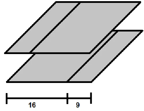
18 top of each other covering the whole area of the mold. Each layer consists of a sheet of 25 x 16 cm and a sheet of 25 x 9 cm and are stacked together in such a way that the separation between those sheets is not hitting a separation of two sheets for a layer above or below (this is represented in
Figure 3.2). The layers are placed such that the carbon fibers are parallel to each other for every layer.
Figure 3.2: Representation of 2 consecutive layers of UD-C/PEI. Each layer consists of a sheet with a width of 9 cm and one with a width of 16 cm
On top of the first ten layers an inert, polyimide Kapton film is placed. The film is placed over the whole length and at the edge of the mold and perpendicular to carbon fibers in the UD-C/PEI. The Kapton film will function as a crack initiator during DCB testing. The width of the Kapton film is 3 cm
and the thickness is 13 μm. Next again sheets of UD-C/PEI are placed in the same way and the same
[image:19.595.169.419.154.346.2]amount as the sheets from the bottom 10 layers. Finally again a 25 x 25 cm metal plate with a thickness of 1 mm coated with marbocoat is placed and a hood to close the mold.
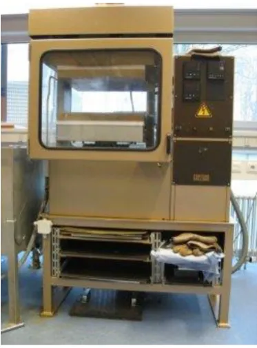
[image:19.595.155.447.500.735.2]19 Figure 3.4: Fontijne TP1000 hot press
Then the Fontijne hot press is set in motion. The temperature is set on 310 °C and when the press reached this value the mold with its content is placed in the press and a force of 50 kN is applied. The application of 50 kN on an area of 25 x 25 cm corresponds to a pressure of 8 bar. After 15 minutes of applying the force the temperature is set on room temperature and a cooling process is started. The mold was cooled under pressure for about 60 minutes. The force was released and the plate of UD-C/PEI was taken out of the mold. Rough edges of the plate were cut off and the plate was cut parallel to the carbon fibers in 12 samples with a width of 2 cm. Next the 12 samples were cut to a length of 20 cm at the edge that does not contain the Kapton film. The average thickness of the samples is 3 mm.
Supramolecular intermediate layer production
In previous research an intermediate layer of SP1 in between plies of UD-C/PEI was made by putting pieces of SP1 on one ply and then pressing another ply on top of it in a press under an elevated temperature. This method did not reached an uniform thickness of the intermediate layer of SP1 in the composite sample. The aim is to make first a supramolecular layer which is of uniform thickness which later can be put in between 2 plies of UD-C/PEI.
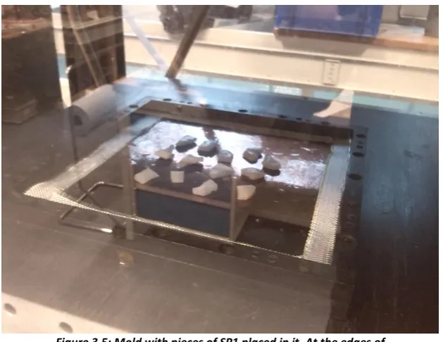
20 at least. To ensure the material is evenly spread over the whole square area and will impregnate the fiber material good enough an excess of material between 10 to 20% is needed. An amount of 17.34 g of SP1 was evenly spread over the 21 x 21 cm square area, meaning an excess of 15.68%. Finally again a thin metal plate with attached to it a marbocoated Kapton foil was placed in the mold and a hood to close it.
Figure 3.5: Mold with pieces of SP1 placed in it. At the edges of the mold the woven fiber material is visible
Next the actual production of the SP1 sheet started. The mold was placed in the press and the temperature was set to 100 °C. When the temperature reached 100 °C the press was set in motion and a force of 100 kN was applied on the mold. An application of 100 kN on an area of 25 x 25 cm corresponds to a pressure of 16 bar. After 15 minutes of applying force the temperature was set at room temperature and a cooling process was started. After 45 minutes the temperature reached a value of 30 °C and the force was taken of the mold. The mold was taken out of the press and the two Kapton foils with in between the SP1 sheet is taken apart. This is left for 3 days before the two foils are released to let the SP1 crystalize. Finally after 3 days are past the SP1 sheet is released from the two foils and is able to cut in pieces with the desired dimensions. The sheet had an average thickness of 0.25 mm and a range from 0.20 mm to 0.28 mm. This was not a problem because the thickness changed gradually over the surface of the sheet so it was possible to cut out layers of SP1 with an uniform thickness and with an deviation of only plus or minus 0.01 mm.
Production of sample with intermediate supramolecular layer
To make a sample with an intermediate supramolecular layer first a composite sample without an intermediate supramolecular layer have to be delaminated into 2 plies. How this is done is elaborated in the paragraph Double Cantilever Beam test of chapter 4. It is chosen to make a sample with an intermediate supramolecular layer from a sample without one instead of making it from 2 separate produced plies. The reason for this is that the sample without an intermediate supramolecular layer can also be tested for its fracture toughness and so results with and without an intermediate layer can be compared afterwards.
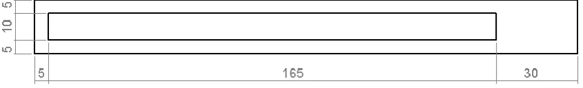
21 is desired a layer of SP1 with certain dimensions is placed on top of 1 ply of the separated composite sample on the side where the delamination took place. Samples are produced with a SP1 intermediate layer thickness of around 0.1 mm or a thickness of around 0.2 mm, depending on how thick the SP1 layer was before it will become an intermediate layer for the final thickness of the intermediate layer. For the samples with a desired SP1 intermediate layer thickness of around 0.1 mm a layer of SP1 with a length and a width of 10 x 165 mm is used. Before this layer is placed it is cleaned with ethanol. This layer is then placed 30 mm from the edge where initially the inert polyimide Kapton foil was placed and 5 mm separated from the other edges, as shown in Figure 3.6, and the other ply is then placed on top. Those 10 x 165 mm SP1 layer are cut out of the produced SP1 sheet as described in Supramolecular intermediate layer production. This sheet has an average thickness of 0.25 mm with a range of 0.20-0.28 mm. The cut out 10 x 165 mm SP1 layer is measured in thickness at 3 different spots evenly spread over the length of the layer. The both delaminated pieces of the composite sample were also measured in thickness on forehand. They were placed back together without a SP1 layer in between and then measured at 9 different spots in the middle of the sample separated 20 mm from each other.
[image:22.595.80.503.302.366.2]
Figure 3.6: Placement of SP1 layer on composite part for thickness of ±0.1 mm
Figure 3.7: Placement of SP1 layer on composite part for thickness of ±0.2 mm
22 Figure 3.8: Press used for production of composite samples containing a SP1 intermediate layer.
Left picture shows whole setup and right picture shows lower half of press. [11]
25 CHAPTER 4:
Double Cantilever Beam test
In this chapter there will be explain how the Double Cantilever Beam (DCB) test works. There will be explained how samples have to be prepared and the set-up is described. Two test methods will be elaborated. The first test method described is a test method used before during previous research and the second test method is a new designed test method specially for testing composite samples containing an intermediate supramolecular layer.
Preparation of sample
[image:26.595.109.490.380.513.2]The Double Cantilever Beam (DCB) test will be used to determine the fracture toughness of the samples. Before the samples are ready to be tested they have to be prepared by gluing on hinges. The hinges are made of stainless steel and are in a shape of a block with a cylindrical hole as can be seen in Figure 4.1. The dimension of the block are 20 x 15 x 15 mm and the radius of the cylindrical hole is 4 mm. The cylindrical hole goes through the both 15 x 15 mm sides. Two hinges will be glued on at both sides of the edge where the Kapton foil crack initiator is present. The hinges as well as the sample will at the glue spot be scrubbed with sandpaper and cleaned with acetone. Then the hinges will be glued on with glue Loctite 401. It is important that the hinges are well aligned to each other and to the edge of the sample.
Figure 4.1: Sample with glued on hinges [3].
26 Figure 4.2: Picture of DCB test set-up showing displacement and delamination length
[image:27.595.71.527.346.714.2]27 Figure 4.4: LabVIEW program used for test method I
Test method I
28 Figure 4.5: Left picture shows moving camera,
right is a schematically representation of camera in motion [3]
The value in red box 1 and the value in the rectangle above red box 1 from the LabVIEW program shown in Figure 4.3 have to be copied in the right two rectangles of red box 1 of the LabVIEW program shown in Figure 4.4, respectively. This are gain/offset values for the force and the displacement so those are zero at the start at the test. Next the LabVIEW program monitoring the measured values is started. Then the lower arm of the DCB test set-up is set in motion. At the machine controlling the movement of this arm the arm is set on a downwards movement of 0.02 mm/s. Due to this movement a force is exerted on the sample and the crack will propagate causing the delamination of the sample. The LabVIEW program measures every second the force and the displacement and saves this data in an array. The camera films the crack propagating and the software of the LabVIEW program analyses the captured pictures. The software recognizes the darker colored crack inside the sample and as a response the camera moves to the point it does not anymore detect any darker contrast in between the white painted sample in its field of view. This process repeats itself also every second and the positon of the camera is also put in a data array. If corrected for a calibration value x0, the x-position of the moving camera equals the delamination
length x. A schematically representation of the moving camera detecting the crack is shown in Figure 4.5. A typical picture of what the software analyses is given in Figure 4.6. The test continues until the crack length is 12-17 cm. This is manually determined during the test by using a ruler. The movement of the lower arm is stopped and is moved back until the LabVIEW program measure a displacement of 0. The LabVIEW program is stopped and the measured data arrays are saved in a text file. Figure 4.4 shows the LabVIEW program and the pictures which will be analyzed as well as an automated drawn Force-displacement graph. The measured data can be used for further analyzing. Finally the lower arm is set in downward motion again until the sample is fully delaminated into 2 plies. From here out a sample with an intermediate supramolecular layer can be made as explained in paragraph
Sample with intermediate supramolecular layer.
[image:29.595.72.524.638.739.2]29
Test method II
Test method I is unreliable to use when testing samples with an intermediate supramolecular layer because at the edges of this layer the paint does not attach well and so darker colored regions in the sample appear which makes it difficult for the software to detect the contrast at the crack. Lots of errors will appear in the measurement of the crack length x making this value incorrect. Therefor another test method had to designed for the case of testing a sample with an intermediate supramolecular layer.
[image:30.595.72.525.344.516.2]This second method is useable to test samples with an intermediate supramolecular and as well samples without an intermediate supramolecular layer. First the sample have to be pre-cracked again and the force and the displacement have to be set on zero in the LabVIEW program as described in paragraph Preparation of sample. This method is based on measuring the angle of rotation α. This angle is measured at the bolt which connects the top hinge to the top arm of the DCB set-up. The bolt is fixed at the hinge with a pin in such a way that the bolt will rotate the same way as the hinge. At the head of the bolt a 90 x 90 mm square cardboard plate is attach in such a way the midpoint of this square and the midpoint of the head of the bolt coincide. The top half of this square is painted white, the lower half of this square is painted black. It is in such a way that the line of separation between the white half and the black half is exactly horizontal when the bolt clamps the sample in the DCB test set-up. All this is shown in Figure 4.7.
30 Figure 4.8: DCB test set-up for test method II
A different camera than the camera used for detecting the crack length is set in front of the 90 x 90 mm square so that the camera captures the whole square well. The software from a LabVIEW program analyzes the footage made by this camera and can detect due to the contrast between the black and the white half the line of separation. Then can it calculate the angle between the line of separation and the lower edge of the field of view of the camera. A screenshot of this is shown in
33
0 10 20 30 40 50
0 10 20 30 40 50 60
Displacement (mm)
F o rce P ( N )
40 50 60 70 80 90 100 110
0 0.2 0.4 0.6 0.8 1 1.2 1.4 1.6 1.8 2
delamination length x (mm)
fr a ct u re t o u g h n e ss GIc ( k J/ m 2) CHAPTER 5:
Results
In this chapter the results of the tests are elaborated. In the first paragraph the designed test method II as described in chapter 3 where a set-up is used wherein the angle is measured is validated. In the second paragraph the effect of the thickness of the intermediate supramolecular layer in the UD-C/PEI sample on the fracture toughness is discussed and the results are placed in context with other adhesives and there physical relations.
Angle measurement validation
Due to the fact test method II, as described in paragraph Double Cantilever Beam test of the previous chapter, is a new developed test method it have to be validated if this method is accurate enough for determining the fracture toughness of the test samples. This is validated by comparing the fracture toughness determined from measurement results of a method I test with the fracture toughness determined from measurement results of a method II test. In both test methods a sample without an intermediate supramolecular layer is tested.
In previous research same samples of UD-C/PEI were tested in a DCB test to determine the fracture toughness with the use of test method I. This previous research was done by J. van de Zand and S.G. Ivanov separately who found both an average value for the fracture toughness of 1.2 kJ/m2 [1,3]. An additional test is performed of a sample of UD-C/PEI running both test method I and II simultaneously (sample 1) followed by 2 tests where a sample of UD-C/PEI is tested with only test method II (sample 2 & sample 3). The average width B of sample 1 equals 19.6 mm, the width of sample 2 equals 19.5 mm and the width of sample 3 equals 19.8 mm. All the three samples have an average thickness of 3 mm (2h = 3.0 mm). A plot of the force versus the displacement and a plot of the fracture toughness versus the delamination length for the test of the sample where both test methods were run simultaneously is given in Graph 5.1. In the right plot of this graph the blue line represents the fracture toughness calculated from the results of test method I, the green line represents the fracture toughness calculated from the results of test method II.
Graph 5.1: F-δ plot and GIc-x plot of UD-C/PEI sample tested with both methods simultaneously (sample 1)
34
0 10 20 30 40 50
0 10 20 30 40 50 60
Displacement (mm)
F o rce P ( N )
40 50 60 70 80 90 100 110
0 0.2 0.4 0.6 0.8 1 1.2 1.4 1.6 1.8 2
delamination length x (mm)
fr a ct u re t o u g h n e ss GIc ( k J/ m 2)
0 10 20 30 40 50
0 10 20 30 40 50 60
Displacement (mm)
F o rce P ( N )
40 50 60 70 80 90 100 110
0 0.2 0.4 0.6 0.8 1 1.2 1.4 1.6 1.8 2
delamination length x (mm)
fr a ct u re t o u g h n e ss GIc ( k J/ m 2)
As the right plot of Graph 5.1 already shows is that the both the test methods give a similar result. For both sample 2 and 3 is also a plot of the force versus the displacement and a plot of the fracture toughness versus the delamination length given. This is shown in Graph 5.2 and Graph 5.3. From the several calculated fracture toughness the mean is determined as well as the variance, the standard deviation and the range. This is set out in Table 5.1.
Graph 5.2: F-δ plot and GIc-x plot of UD-C/PEI sample tested with method II (sample 2)
Graph 5.3: F-δ plot and GIc-x plot of UD-C/PEI sample tested with method II (sample 3)
Mean GIc (kJ/m2) Variance (kJ2/m4) STD (kJ/m2) Range (kJ/m2) Sample 1
- method I 1.1584 0.0031 0.0553 1.0686 – 1.2888
- method II 1.2030 0.0021 0.0463 1.0866 – 1.3072
Sample 2
- method II 1.1914 0.0024 0.0493 1.1085 – 1.2828
Sample 3
[image:35.595.87.524.152.344.2]- method II 1.2193 0.0022 0.0473 1.1063 – 1.3064
35 As the results from this tests show, samples which are tested with test method II give same values for the fracture toughness as test method I. The mean fracture toughness determined with test method II only differ a maximum of 1.61% from the average fracture toughness of 1.2 kJ/m2 found by J. van de Zand and S.G. Ivanov so this test method seems validated.
Influence of the thickness
The effect of the thickness of the intermediate supramolecular layer in the UD-C/PEI sample on the fracture toughness is determined. Several samples were tested with a DCB test using test method II. The samples varied to each other in width of the sample and in thickness of the intermediate supramolecular layer. If a sample with an intermediate supramolecular layer was produced, as described in Production of sample with intermediate supramolecular layer of chapter 3, the thickness of the intermediate supramolecular in this sample was determined. The sample was tested in the DCB test set-up and was after the test fully delaminated. The outside of the sample was cleaned with acetone and it was put back in the hot press in the way how it is described in also Production of sample with intermediate supramolecular layer of chapter 3. The sample will be healed in the press at 0.2 bar but the temperature and press time will be varied in comparison with the production to decrease the thickness of the intermediate supramolecular layer. Raising the temperature and/or the press time creates a flow of SP1 out of the sample and so decreasing the thickness of the intermediate layer. Temperature is in the range from 120 °C to 140 °C and healing time from 10 to 50 minutes. The used parameters for each healing cycle is not given explicitly, only the end result of the healing cycle to the thickness of the intermediate supramolecular layer is of importance. Samples can after a healing cycle be prepared to be tested again and the process of decreasing the intermediate supramolecular layer can be also repeated after an additional test.
The results of tests of 5 different samples from which several of them have been tested for different thicknesses are shown in Table 5.2. In this graph the layer thickness is the mean value of the intermediate supramolecular layer measured at 9 different spots evenly spread over the centerline of the sample. GIc is the mean of the fracture toughness calculated from each test’s measurement
data. STD is the standard deviation of the fracture toughness and the range is the minimum and maximum value for each calculated fracture toughness. In Graph 5.4 the 4 different calculated values of the fracture toughness for sample 3 is shown. For clarity, the mean fracture toughness GIc is
36 Sample # Layer thickness (mm) GIc (kJ/m2) STD (kJ/m2) Range (kJ/m2)
2 0.081 0.2966 0.1303 0.143 – 0.573
2 0.101 0.3723 0.0936 0.225 – 0.531
2 0.120 0.5132 0.0679 0.403 – 0.631
2 0.141 0.7932 0.0240 0.709 – 0.826
2 0.149 0.8456 0.0844 0.682 – 1.070
3 0.170 0.8694 0.0798 0.674 – 0.997
3 0.141 0.8899 0.1220 0.637 – 1.084
5 0.140 0.9004 0.0656 0.833 – 1.058
4 0.148 0.9306 0.0819 0.745 – 1.065
2 0.170 0.9706 0.1058 0.790 – 1.148
3 0.200 1.2154 0.1218 1.015 – 1.393
1 0.185 1.3451 0.1080 1.107 – 1.546
1 0.205 1.4098 0.0989 1.234 – 1.559
3 0.218 1.4219 0.1337 1.100 – 1.648
[image:37.595.114.467.365.648.2]1 0.240 1.6406 0.0629 1.488 – 1.731
Table 5.2: Results of DCB tests of UD-C/PEI samples with intermediate supramolecular layer on fracture toughness
Graph 5.4: Fracture toughness of sample 3 with different thickness. Red: 0.218 mm, Blue: 0.200 mm, Green: 0.141 mm, Turquoise: 0.170 mm
The values of the layer thickness and the fracture toughness GIc are also set out in Graph 5.5. The
standard deviation for each value of the fracture toughness is also present in this graph. The software program MatLab calculated a linear fit for the values of the fracture toughness and this is also plotted in the graph. The function of this linear fit is: GIc = 8.6246 t – 0.4233, where t represents
the layer thickness in mm and GIc is in kJ/m2.
20 30 40 50 60 70 80 90
0 0.2 0.4 0.6 0.8 1 1.2 1.4 1.6 1.8 2
Delamination length [mm]
37 S.G. Ivanov found a fracture toughness of 1.1 kJ/m2 for an UD-C/PEI sample with an intermediate supramolecular layer of 0.15-0.20 mm which is in accordance with the test results of this research. From the function for the linear fit the layer thickness needed to reach a fracture toughness of 1.2 kJ/m2 so that at the intermediate supramolecular layer the ability to resist fracture when a crack is present is the same as a sample of UD-C/PEI without an intermediate supramolecular layer can be determined. This value for this layer thickness is 0.188 mm. The test results shows linear increasing behavior for the fracture toughness as a function of the layer thickness. This is in accordance with the research of Shantanu R. Ranade et al. who found for adhesive bonds the relation between the fracture toughness and the layer thickness (bondline thickness is his report) as shown in Graph 5.6
[9]. For relative low values of the bondline thickness the fracture toughness shows linear increasing behavior until a certain maximum point from where the fracture toughness decreases by increasing bondline thickness until a point the fracture toughness becomes a steady value. The calculated fracture toughness values from the tests are in the linear increasing area of the fracture toughness- bondline thickness relation.
Graph 5.5: Plot of fracture toughness vs layer thickness
0 0.05 0.1 0.15 0.2 0.25 0.3
0 0.5 1 1.5 2 2.5
Layer thickness [mm]
38 Graph 5.6: Plot of relation between bondline thickness and fracture toughness for adhesive bonds [15]
Comparing the values of the fracture toughness of the SP1 intermediate layer with the values of the fracture toughness of other adhesives shows that the fracture toughness of the SP1 intermediate layer is relative high. Most adhesive shows a maximum fracture toughness between 0.5-1.0 kJ/m2 [10]. The relation between the fracture toughness and the adhesive layer thickness for 3 other adhesives in the linear increasing area is shown in Graph 5.7. The 3 adhesives are tuff-ply, FM 73 and FM 300 and all work as an intermediate adhesive layer in unidirectional carbon fibre reinforced epoxy material (CFRP). Compared with those values SP1 also shows relative high linear progress of fracture toughness for its relative low adhesive layer thickness.
39 CHAPTER 6:
Conclusions and Recommendations
In this chapter the conclusions of the findings from this research are drawn with respect to the goals of the research. Also some recommendations are given for the application of SP1 and for additional research.
Conclusions
In chapter 1 Introduction of this bachelor assignment three goals where determined. The first goal was to design a production method for samples with an intermediate supramolecular layer so that a uniform thickness is achieved. The second goal was to design a test method from which the measurement data is reliable. And the third goal was to investigate the effect of the thickness of the intermediate supramolecular in the composite samples to the interlaminar fracture toughness. With respect to those goals the following conclusions can be drawn:
- The production method designed to produce UD-C/PEI samples with an uniform intermediate supramolecular layer thickness is usable. However the produced sheet of SP1 as described in chapter 3 was not uniform in thickness over the whole surface of the sheet, there were uniform thickness regions in this sheet which makes in able to so cut out uniform layers of SP1 so eventually from this a UD-C/PEI sample with an uniform intermediate supramolecular layer thickness can be made.
- The aim to produce a sheet of SP1 with a thickness of 0.3 mm was overachieved. A lower average thickness of 0.25 mm was reached for the produced sheet of SP1. The pressure used during the production was relative so high that the woven fiber material which had to be impregnated by SP1 became compressed leading to a lower thickness.
- The designing of test method II to measure reliable data for DCB tests of samples with an intermediate supramolecular layer was successful. The test method II was validated in comparison to the already proven to be useable test method I. Both test methods showed the same results for the fracture toughness of UD-C/PEI samples without an intermediate supramolecular layer. Besides the test method II is reliable to use for testing of samples with an intermediate supramolecular layer the method is less time consuming because samples do not have to be painted white.
- An intermediate supramolecular layer thickness of 0.188 mm in UD-C/PEI is needed to ensure the same interlaminar fracture toughness for samples with and without and intermediate supramolecular layer.
- The relation between the fracture toughness and the thickness of the intermediate supramolecular layer in UD-C/PEI shows linear increasing behavior of the fracture toughness for the tested thicknesses of the intermediate supramolecular layer. This is in agreement with the behavior of other adhesives.
40
Recommendations
The results from the research led to some recommendations for the application of SP1 and some recommendation for further research. Those recommendations are numerated below:
- There can be thought of designing a self-healing composite material existing of alternating layers of UD-C/PEI and SP1. UD-C/PEI will maintain the strength of this material because SP1 itself is very weak compared to UD-C/PEI and has a relative low elastic modulus. The SP1 provides then self-healing capability. When this material then becomes delaminated this can be healed applying heat under some low pressure. This can be done by for example pressing a hot metal rod to the crack of the delamination for a certain time. If designing this material to have an interlaminar fracture toughness which is the same for both types of layer a thickness of the SP1 layer of at least 0.188 mm is needed.
41
References
[1] Damage healing of a supramolecular polymer interlayer in thermoplastic composite laminates, S.G. Ivanov et al.
[2] Picture copied from Self-healing in action, Anton W. Bosman
[3] Picture copied from Automated Double Cantilever Beam test system, J. van de Zand [4] Picture copied from
http://upload.wikimedia.org/wikipedia/commons/e/e7/Fracture_modes_v2.sv [5] Edited picture from Automated Double Cantilever Beam test system, J. van de Zand
[6] Griffith, A. A. (1921), "The phenomena of rupture and flow in solids", Philosophical Transactions of the Royal Society of London, A 221: 163–198,doi:10.1098/rsta.1921.0006. from:
http://en.wikipedia.org/wiki/Fracture_mechanics#cite_note-1
[7] Irwin, G.R. and J.A. Kies, Critical energy rate analysis of fracture strength. Welding Research Supplement, 1954. 19: p. 193-198.
[8] INSTANTANEOUS EVALUATION OF J AND C*, Anthony J, and Paul C. Paris
[9] A tapered bondline thickness double cantilever beam (DCB) specimen geometry for combinatorial fracture studies of adhesive bonds, Shantanu R. Ranade et al., 20 august 2014
[10] Adhesive thickness effects of a ductile adhesive by optical measurement techniques, R.D.S.G. Campilho et al, 8 December 2014
[11] Picture copied from Damage healing in composite materials - Creating an experimental setup, Casper Flim, 11 april 2013
[12] Edited picture from Damage healing in composite materials - Creating an experimental setup, Casper Flim, 11 april 2013
[13] Self-healing in action, Anton W. Bosman
[14] Supramolecular polymers at work, Anton W. Bosman et at., April 2004
[15] Picture copied from A tapered bondline thickness double cantilever beam (DCB) specimen geometry for combinatorial fracture studies of adhesive bonds, Shantanu R. Ranade et al., 20 august 2014
![Figure 2.2: Sample of a DCB test. The hinges on the left end are the place where the sample will be clamped [3]](https://thumb-us.123doks.com/thumbv2/123dok_us/9814492.482699/11.595.77.517.509.710/figure-sample-dcb-test-hinges-place-sample-clamped.webp)
![Figure 2.4: Partially delaminated sample with representation of parameters [5]](https://thumb-us.123doks.com/thumbv2/123dok_us/9814492.482699/12.595.91.504.265.471/figure-partially-delaminated-sample-representation-parameters.webp)
![Figure 2.5: J-integral approach on a DCB test sample by J. and C. Paris [8]](https://thumb-us.123doks.com/thumbv2/123dok_us/9814492.482699/14.595.77.526.334.455/figure-j-integral-approach-dcb-test-sample-paris.webp)