University of Warwick institutional repository
This paper is made available online in accordance with publisher policies. Please scroll down to view the document itself. Please refer to the repository record for this item and our policy information available from the repository home page for further information.
To see the final version of this paper please visit the publisher’s website. Access to the published version may require a subscription.
Author(s:
Article Title: Measuring inequality in a cross-tabulation with ordered categories: from the Gini coefficient to the Tog coefficient
Richard Lampard
Year of publication: 2000
Measuring inequality in a cross-tabulation with ordered
categories: from the Gini coefficient to the Tog coefficient
[Pre copy-editing version: January 2000]
Richard Lampard
Address:
Department of Sociology,
University of Warwick,
Gibbet Hill Road,
Coventry,
WEST MIDLANDS CV4 7AL.
Tel.:
(01203) 523130
Fax:
(01203) 523497
e-mail:
[email protected]
Author’s bionote
Richard Lampard is a Lecturer in the Department of Sociology, University of
Measuring inequality in a cross-tabulation with ordered
categories: from the Gini coefficient to the Tog coefficient
Abstract
This paper introduces the Tog coefficient, which can be used to measure the level of inequality in a
cross-tabulation of two ordinal-level variables. The Gini coefficient is a standard measure of income
inequality which has been adapted by other authors for use in different contexts such as the
measurement of health inequalities and the quantification of occupational segregation; the Tog
coefficient represents a further stage in this process of development. The paper outlines the construction
of the Tog coefficient and illustrates this using a social mobility table based on data from the 1972
Oxford Mobility Study. The trend in social mobility-related inequality as measured by the Tog
coefficient is compared with the findings of Goldthorpe et al. based on odds ratios. A more elaborate
application of the Tog coefficient uses a variety of data relating to the similarity of spouses’ class
backgrounds to demonstrate the existence of a long-term decline in the level of inequality in British
society.
Introduction
Lorenz curves and the Gini coefficient are standard approaches to the depiction and
quantification of income inequality (Atkinson 1983, Marsh 1988). In their basic forms
these measures are constructed from univariate, interval-level data, such as the
incomes of the members of a population. However, there is a straightforward
extension of the way in which the Gini coefficient operationalizes inequality which
those found in a social mobility table. This paper introduces this related measure, the
Tog coefficient.
The paper starts with a brief discussion of the construction of Lorenz curves and the
Gini coefficient, and of the ways in which they have been adapted and developed by
other authors. One of these adaptations then acts as a signpost towards the way in
which the Tog coefficient measures the inequality in a cross-tabulation based on two
ordinal-level variables. The construction of the Tog coefficient is illustrated using a
social mobility table as an example, and the coefficient is then defined in
mathematical terms. The Tog coefficient and its characteristics are then assessed, with
reference to debates regarding the measurement of inequality and the evaluation of
trends in social mobility, and using odds ratios as a particular point of comparison.
Finally, the Tog coefficient is applied to data on husbands’ and wives’ class
backgrounds within an analysis of long-term trends in inequality in Britain.
Lorenz curves and the Gini coefficient: construction and developments
To construct a Lorenz curve in the context of income inequality, incomes are first
ordered from lowest to highest. The Lorenz curve is obtained by plotting cumulative
income shares against cumulative percentages of the population. For example, if the
20% of the population who have the lowest incomes collectively have a 5% share of
the total income, the point (20%, 5%) lies on the Lorenz curve. The figure of 5% can
be seen to correspond to a shortfall of 15% relative to a situation of perfect equality.
from (0%, 0%) to (100%, 100%), which passes through (20%, 20%). The Gini
coefficient summarises the shortfall in income across all cumulative percentages of
the population; it does this by comparing the area between the Lorenz curve and the
line of perfect equality with the total area beneath the line of perfect equality. This
leads to a value of between 0 and 1, with 0 indicating perfect equality and 1 the
maximum level of inequality (i.e. where one individual has all the income!)
The Gini coefficient has also been used to quantify inequality in other contexts. For
example, Le Grand and Rabin (1986) have used it to measure inequality in longevity.
In this context, ages at death are ordered from lowest to highest, and the Lorenz curve
is generated by plotting cumulative years lived against cumulative percentages of the
people who have died. For example, the 10% who died youngest may have only had a
5% share in the total number of years lived. More recently, variants of the Gini
coefficient have been applied to the measurement of inequality corresponding to
categorical variables (such as occupation) as well as interval-level variables (such as
income and age at death). Specifically, occupational gender segregation has been
measured in this way (Hutchens 1991, Boisso et al. 1994, Lampard 1994). In this
context, occupations are ordered from the occupation with the lowest proportion of
women in it to the occupation with the highest proportion of women in it. The Lorenz
curve is generated by plotting the cumulative percentage of women in occupations
against the cumulative percentage of people of either sex in occupations. A variant of
the Gini coefficient is once again generated with reference to the area between the
Further developments of the Lorenz curve and Gini coefficient have extended them to
multivariate situations. Koshevoy and Mosler (1996) consider inequality with respect
to multiple outcomes, whereas authors such as Boisso et al. (1994) and Watts (1997)
look at multidimensional occupational segregation with regard to factors such as
gender and ‘race’. Yao and Liu (1996) decompose income inequality by introducing
additional, explanatory variables such as occupation. However, it is Hellevik (1997)
who uses these measures of inequality in the way which comes closest to the approach
developed in this paper.
Measuring inequality in a cross-tabulation based on two ordinal-level variables
Hellevik (1997) examines the relationship between class background and recruitment
to higher education. This in effect involves the analysis of an N by 2 cross-tabulation,
where N is the number of classes and there are two outcomes: recruitment or
non-recruitment to higher education. The classes can be put into order according to the
levels of recruitment to higher education from within them in much the same way as
occupations can be ordered according to the gender balance within them. Thus
Hellevik’s analysis in practice has much in common with analyses of occupational
segregation.
However, educational attainment need not be viewed simply in terms of recruitment to
higher education. Thus an analysis of inequality in educational attainment might also
distinguish between individuals who left education at the minimum school-leaving
were not recruited to higher education. Such an analysis would then focus on an N by
3 cross-tabulation, with both class and education being ordinal-level variables.
The original contribution of this paper is to develop the Lorenz curve and Gini
coefficient in such a way as to allow the level of inequality in a cross-tabulation of the
above sort to be quantified. Since the coefficient introduced by this paper measures
inequality with respect to two, ordinal-level variables, and is a variant of the Gini
coefficient, it is referred to using an appropriate abbreviation, i.e. as the Tog
coefficient.
The key way in which the logic behind the construction of the Gini coefficient is
extended to give the Tog coefficient is very straightforward. The process of
cumulation which is central to the generation of the Lorenz curve is simply applied to
both the variables in a cross-tabulation rather than just to one of themii. This results in
something akin to a set of Lorenz curves, which collectively form a surface. Just as
the Gini coefficient is based on the area between the Lorenz curve and the line of
perfect equality, the Tog coefficient is based on the volume bounded by the ‘Lorenz
surface’ and the surface of perfect equality.
An understanding of the above may perhaps be facilitated by a consideration of
Hellevik’s analysis and the extension to it suggested earlier. In Hellevik’s analysis one
of the points on the Lorenz curve is defined by the number of individuals recruited
into higher education from the bottom two classes plotted against the total number of
individuals in the bottom two classes. In the suggested extension to his analysis, one
from the bottom two classes who either were recruited into higher education or carried
on to some form of post-compulsory education plotted simultaneously against both the
total number of individuals in the bottom two classes and also the total number of
individuals who were recruited into higher education or carried on to some form of
post-compulsory education.
An example: measuring inequality in a (social) mobility table
In this section a classic social mobility table is used to further illustrate the process of
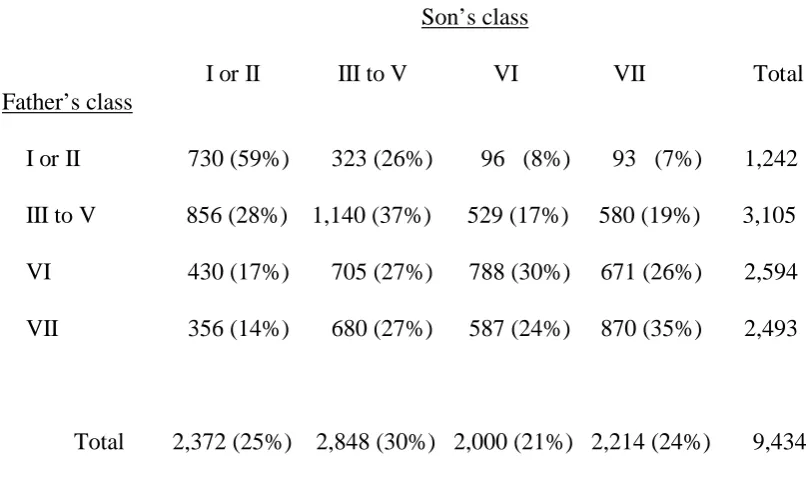
construction of the Tog coefficient. Table 1 relates to father-to-son intergenerational
social mobility and is based on data from the 1972 Oxford Mobility Study
(Goldthorpe et al. 1987). It is consistent with one of the key mobility tables arising
from that study (1987: 105), but the number of categories is smaller to simplify the
exampleiii.
[Insert table 1 about here]
It can be seen from table 1 that there is a shortfall in the percentage of sons with
fathers in Class VII who are in Classes I or II (14% compared with 25% of all sons). A
similar, though slightly smaller, shortfall (17% compared with 25%) exists for the
sons of fathers in Class VI. The first stage in the construction of the Tog coefficient is
the cumulation of the values in each of the columns from bottom to top, which results
in table 2. It can be seen from table 2 that 15% of sons with fathers in Classes VI or
[Insert table 2 about here]
The next stage in the construction of the Tog coefficient is the cumulation of the
values in each of the rows from left to right, which gives table 3. Table 3 thus shows
the percentage of sons whose fathers are in classes of a specified level or lower who
are themselves in classes of a (second) specified level or higher. For example, 43% of
sons whose fathers are in Classes VI or VII are themselves in Classes I to V, a
shortfall of 12% compared to the figure for all sons (55%).
[Insert table 3 about here]
[Insert figure 1 about here]
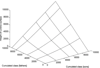
Each of the values in table 3, when plotted simultaneously against the corresponding
cumulative column total and the corresponding cumulative row total, is a point on the
‘Lorenz surface’ for table 1. This surface is shown graphically in figure 1. The amount
of inequality in table 1 can be viewed as the volume between this surface and the
surface that would have been obtained in a situation of perfect equality, i.e. one where
father’s class and son’s class were unrelated. This second surface corresponds to the
values given in table 4. Thus the Tog coefficient measures the inequality in table 1 by
summarising the shortfalls in the values in table 3 relative to the values in table 4.
[Insert table 4 about here]
The mathematics of the calculation of the volume between the surfaces is described
size involved, the volume can be shown to be 0.0248. This value then needs to be
compared with the value corresponding to the maximum possible level of inequality
that could have been observed in the table (given its marginal frequencies; see table 5
below). This second volume can be shown to be 0.0714. Thus the value of the Tog
coefficient for table 1 is 0.0248/0.0714 = 0.347. Note that a value of 0 would indicate
perfect equality, and a value of 1 would indicate the maximum possible level of
inequality.
The mathematics of the Tog coefficient
Suppose that a cross-tabulation has I rows and J columns. Let Fij be the number of
cases in the cell which is in the i-th row and the j-th column of the cross-tabulation.
Then Tij, the total number of cases in the cells which lie both within the first r rows
and also within the first c columns of the cross-tabulation, is as follows:
r c Trc = Σ Σ Fij
i=1 j=1
In a situation of perfect equality, i.e. one where there is no relationship between the
two variables defining the cross-tabulation, the expected value of Trc (which is
denoted as Erc) is as follows:
1 r c Erc = ── Σ Ri Σ Cj
where Ri is the total number of cases in the i-th row, Cj is the total number of cases in
the j-th column and N is the total number of cases in the cross-tabulation. (Note that
tables 3 and 4 show the values of Trc and Erc corresponding to table 1).
The shortfall in Trc relative to the value expected if there were no relationship is thus
as follows:
Drc = (Erc -Trc)
To generate a Gini coefficient from a Lorenz curve one calculates the area between
the Lorenz curve and the straight line corresponding to perfect equality, and expresses
this area as a proportion of the whole area beneath the perfect equality line. The
equivalent process here starts with an assessment of the size of the volume (V)
between the surfaces defined by Trc (r = 0 to I; c = 0 to J) and by Erc (r = 0 to I; c = 0
to J). Note that for r = 0 and/or c = 0, Trc and Erc take the value 0. Volume V can be
broken down into smaller volumes defined in terms of pairs of neighbouring rows and
1 I J
V = ── Σ Σ ¼ RrCc (Drc + D(r-1)c + Dr(c-1) + D(r-1)(c-1)) N3 r=1 c=1
Note that the above equation takes account of the effect of the sample size, N, on the
volume.
At first sight, the obvious point of comparison for V is the volume underneath the
surface defined by the values of Erc, which seems to be the natural equivalent to the
area under the perfect equality line in the calculation of the Gini coefficient. However,
marginal frequencies place constraints on the patterns of inequality which are possible
in a table (see table 5 below), and it turns out that a consequence of using the obvious
point of comparison would be that the maximum possible value of the Tog coefficient
was not 1 (and that it varied according to the specific cross-tabulation being
examined).
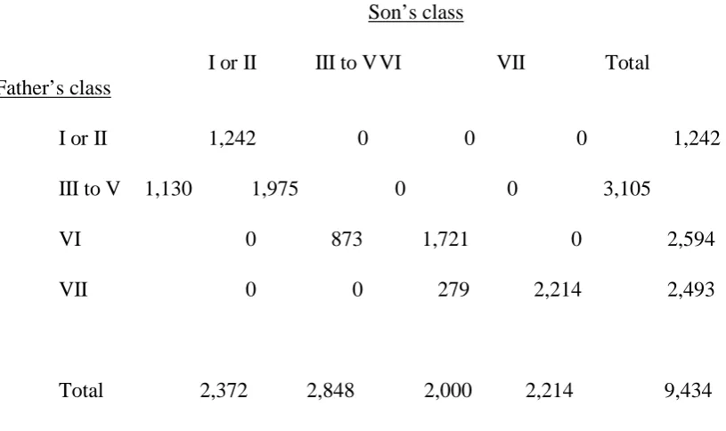
Volume V thus needs to be evaluated relative to the maximum possible value that it
could have taken (Vmax). The simplest way of calculating this maximum value is to
identify the cross-tabulation to which it corresponds, i.e. the cross-tabulation with the
strongest possible ordinal pattern of association between the variables given the
observed marginal frequenciesiv. For the example being considered here, the relevant
cross-tabulation is table 5.
As noted earlier, the value of volume V for table 1 is 0.0248, and the value (Vmax) for
table 5 is 0.0714. Hence the value of the Tog coefficient is as follows:
Tog = V = 0.0248 Vmax 0.0714
= 0.347
Note that Vmax for a symmetric table with k rows and columns and with uniform
marginal frequencies can be shown to be given by the formula (k2-1)/12k2. Thus for a
4x4 table of this sort, Vmax would be 15/192, or 0.078125. The effect of the marginal
frequencies in table 1 is thus to reduce Vmax from 0.078125 to 0.0714.
An assessment of the Tog coefficient and its characteristics
Having introduced the Tog coefficient, it seems appropriate to assess its value and
discuss its distinctive characteristics, in part with reference to other measures which
have been applied to cross-tabulations based on ordinal-level variables. Such other
measures include measures of association for ordinal-level variables, e.g. Gamma and
Tau-b (Loether and McTavish 1993: 219), and odds ratios, as used by authors such as
Goldthorpe et al. (1987)v. The discussion that follows focuses on odds ratios as a
point of comparison.
The most obvious advantage of the Tog coefficient as a measure of inequality is that it
shares the underlying logic of the Gini coefficient, inasmuch as it views inequality as
being related to the shortfall in some desirable outcome experienced by the more
disadvantaged part of the population. In itself this is not a unique quality, but both the
disadvantaged/advantaged distinctions, rather than just with respect to a specific
cut-off point. No doubt the Tog coefficient shares with the Gini coefficient other desirable
qualities as a measure of inequality (Marsh 1988: 88), as well as idiosyncrasies
(Atkinson 1983). A corollary of the Tog coefficient’s relationship to the Gini
coefficient is that by using both coefficients inequalities documented by data at
different levels of measurement can be quantified in a parallel way.
However, the fact that the Tog coefficient is derived from categorical data does result
in some characteristics that are not shared with the Gini coefficient. One of these is
the sensitivity of the Tog coefficient to the number and range of categories used, given
a degree of internal heterogeneity within categories. Aggregating two rows or two
columns of a cross-tabulation is likely to reduce the value of the Tog coefficient, as
some of the fine detail of the inequality represented by the ‘Lorenz surface’ will be
lostvi. Thus to allow the Tog coefficient to capture the full extent of the inequality in a
situation, categories should where possible be disaggregated to minimise internal
heterogeneity. In practice, however, a thin spread of cases across a cross-tabulation
with a large number of rows and columns might decrease the precision of the Tog
coefficient. Note that the sensitivity of the Tog coefficient to the categories used is
shared with other measures of inequality or association applied to cross-tabulations; it
reflects the structure of the data analysed rather than the measure itself.
Another feature of the Tog coefficient can be viewed as an advantage or as a
disadvantage, depending on one’s theoretical agenda and how one conceptualises
inequality. Differences between the marginal distributions in two cross-tabulations
ways. More specifically, multiplying the values in one of the columns or rows of a
cross-tabulation by a constant does not affect the odds ratios but does affect the Tog
coefficient. The issue of marginal distributions is central to the work of Hellevik
(1997) mentioned earlier in the paper, and also ties in with the debate between
Saunders (1989) and Goldthorpe and others regarding the evaluation of trends in
social mobility.
Hellevik (1997: 377) argues that while measures such as odds ratios can capture
association or effect, inequality or unrepresentativity must be captured by measures
like the Gini coefficient. He notes the absence of explicit definitions of inequality in
the class inequality literature, and suggests that when one is interested in equality of
outcome (in relation to the acquisition of some good) rather than equality of
opportunity (i.e. equality in the allocation process) ‘the relevant measures would seem
to be those which compare the distributions of the good with that of the population’
(Hellevik 1997: 389).
Hellevik further suggests (1997: 378) that the findings of stability in the levels of
various forms of inequality of a number of authors including Goldthorpe et al. (1987)
to an extent reflect the impact (or lack of impact) of marginal distributions on their
choices of measure. This echoes Saunders’ long-standing critique of the findings of
Goldthorpe et al. in relation to social mobility, which argues that an emphasis on
trends in relative mobility (as measured by odds ratios) inappropriately screens out the
The above debate highlights the specificity of what is measured by odds ratios.
Analysing trends in social mobility using odds ratios treats the occupational class
categories as fixed points of reference, and focuses on the pattern of movement
between classes of origin and classes of destination. However, when one uses the Tog
coefficient to look at a social mobility table one is focusing on something different.
More specifically, the Tog coefficient has as its point of reference the existence of a
hierarchy (or ranking) of occupations which may vary over time (as opposed to
categories with fixed meanings). As occupational categories expand and contract, or
change order, the hierarchy changes accordingly, and hence so may the Tog
coefficient. When applied to social mobility tables, the Tog coefficient summarises
the degree of inequality in the way that occupations within this (shifting) hierarchy are
distributed according to the positions of individuals within the (shifting) hierarchy of
class background.
A more straightforward advantage of the Tog coefficient as compared to odds ratios is
that the Tog coefficient is a single value, whereas the pattern of association in a
cross-tabulation generates a number of odds ratios dependent on the number of rows and
columns. However, this advantage is one shared with most measures of association.
Furthermore, boiling down the pattern in a cross-tabulation to a single measure of
inequality inevitably involves some simplifying assumptions about the underlying
process which generated the pattern in the cross-tabulation. The patterns in the
intergenerational mobility tables analysed by Goldthorpe et al. and other authors are
typically multidimensional, reflecting specific forms of occupational inheritance and
agricultural/industrial distinctions as well as a central relationship between fathers’
such a cross-tabulation, the ‘Lorenz surface’ underpinning the Tog coefficient can be
‘bumpy’, and does not necessarily share the non-decreasing gradient of the Lorenz
curve.
For some superficially ordinal-level variables such as occupational class it may not be
clear what the correct ordering of the categories is. Arranging the categories
inappropriately may once again lead to a bumpy ‘Lorenz surface’. The obvious
solution is to order the categories in such a fashion as to maximise the Tog coefficient,
but this does not necessarily ‘iron out’ all the bumps in the surface. However, in many
cross-tabulations based on ordinal-level variables the above situations will not arise,
and even if they do it is not clear that they invalidate the Tog coefficient as a measure
of inequality.
Measures of inequality such as the Tog coefficient are typically used to compare
levels of inequality between different times or different places. However, where the
Tog coefficient is used to measure the levels of inequality in cross-tabulations derived
from samples, it is clearly susceptible to sampling error. The statistical significance of
the difference between two Tog coefficients should therefore be assessed in terms of
their standard deviations. It seems likely that the derivation of the sampling
distribution of the Tog coefficient would be an awkward task, but standard deviations
of comparable measures have been estimated empirically using bootstrap and
jackknife techniques (e.g. Boisso et al. 1994). Thus it is perhaps simplest to use
bootstrap estimates of standard deviations to assess the statistical significance of
For example, Goldthorpe et al. examined trends in social mobility. If table 1 is
subdivided according to son’s birth cohort in a broadly comparable way to their
analysis (Goldthorpe et al. 1987: 69), Tog coefficients of 0.329 for sons born in the
period 1908-1927 and 0.375 for sons born in the period 1928-1947 are obtained. An
estimated standard deviation (based on 25 bootstrap samples; see Efron 1979) was
calculated for each of the coefficients; the estimate was 0.015 in each case.
Combining these gives an estimated standard deviation of 0.021 for the difference
between the two coefficients, and, based on a z-test, the difference would thus (just)
appear to be statistically significant at the 5% level.
The implication of the above is that the level of inequality is greater within the latter
set of birth cohorts. At first sight this seems to contradict Goldthorpe et al.’s finding
of ‘constant social fluidity’. However, ‘social fluidity’ as measured by odds ratios and
‘inequality’ as measured by the Tog coefficient are mathematically different from each
othervii. Thus it is not paradoxical for inequality to be increasing while social fluidity
remains constantviii. Whether it is fluidity or inequality which is of greater conceptual
importance is a matter for theoretical debate.
An application of the Tog coefficient: trends in assortative marriage for class background
The relationship between husbands’ and wives’ socio-economic characteristics can be
used as a source of information about the social order (Prandy and Bottero 1998), and
the strength of the relationship has often been seen as a measure of societal openness
number of sources are used to examine long-term shifts in societal openness in
Britainix. One of the problems with such an analysis is the marked changes in
occupational structure which have taken place. However, if one is prepared to make a
few (rather strong) assumptionsx, the Tog coefficient can be validly used to compare
data from different periods with varying occupational structures, even if the
occupational class classifications used differ. In the analysis that follows all the
cross-tabulations used to generate the Tog coefficients have the same number of rows and
columns (four of each), in an attempt to reduce the impact on the coefficients of the
form of the cross-tabulations.
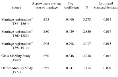
Table 6 shows the Tog coefficients for cross-tabulations of husbands’ and wives’ class
backgrounds corresponding to marriages starting during periods of time stretching
from the mid-nineteenth to the mid-twentieth centuries. The data analysed come from
three sources. The first of these covers the period 1839-1914 and makes use of
occupational information from marriage registration records (Miles 1993). The second
source is the 1949 Mobility Study by Glass (1954), with the data used being those
relating to the marriages of male respondents. The third source is the Oxford Mobility
Study of 1972 (Goldthorpe et al. 1987)xi.
The Tog coefficients in table 6 indicate that the level of inequality in society, as
echoed by the similarity of spouses’ class backgrounds, declined between the
mid-nineteenth and mid-twentieth centuries. The estimated standard deviations (each based
on 25 bootstrap samples) suggest that this pattern is statistically significant; each of
the last three Tog coefficients is significantly lower than each of the first two
fourth coefficientsxii. The departures from the broad downward trend could be
genuine, or an artefact of the different data sources used, and they may also reflect
sampling errorxiii. Overall, the Tog coefficient shows a growth in societal openness
between the mid-nineteenth and mid-twentieth centuries, judged in terms of the
mixing of class backgrounds within marriages.
[Insert table 6 about here]
Conclusion
This paper has introduced the Tog coefficient, a measure which can be used to
quantify the inequality in a cross-tabulation of two ordinal-level variables. Many
measures can be used to summarise the pattern visible in a cross-tabulation; the Tog
coefficient’s distinctive feature is that it summarises the pattern in a similar fashion to
the way in which the Gini coefficient measures inequality with respect to univariate,
interval-level data. Thus, for example, the Tog coefficient summarises the pattern in a
different way to odds ratios; trends in the Tog coefficient across a series of
cross-tabulations may consequently differ from trends in odds ratios. The relative merits of
the Tog coefficient and odds ratios depend upon the task to be carried out; the author
shares Hellevik’s view that a measure like the Tog coefficient is more appropriate for
assessing ‘inequality’, but would tend to agree with Goldthorpe et al. that odds ratios
are better measures of ‘fluidity’.
This paper’s use of odds ratios as a point of comparison, together with the author’s
impression that the Tog coefficient’s potential value is restricted to quite a limited
range of analyses and substantive topics. It is therefore important to reiterate the point
that the Tog coefficient may be of value to any analysis of cross-tabulated
ordinal-level data. However, as is inevitable with a new measure, further reflection and
investigation is needed to establish under what circumstances it is more appropriate
than any of the range of competing measures.
Acknowledgements
The author would like to thank the anonymous referees for their helpful comments on
this paper. The author would also like to thank Andrew Miles for allowing the
marriage registration dataset to be used in this paper. Data from the two mobility
studies (London School of Economics and Political Science et al. 1974, Oxford Social
Mobility Group 1978) were obtained via the Data Archive at the University of Essex,
whom the author would like to acknowledge along with the original depositors of the
data, D.V. Glass, A.H. Halsey and J.H. Goldthorpe. In addition, material from the
1949 Mobility Study is Crown Copyright and has been used by permission of the
Office for National Statistics. The researchers who carried out the original collection
and analyses of the data bear no responsibility for the further analyses and
References
Atkinson, A.B. (1983) The Economics of Inequality [Second edition] (Oxford: Oxford
University Press).
Blackburn, R.M., Jarman, J. and Siltanen, J. (1993) The analysis of occupational
segregation over time and place: considerations of measurement and some new
evidence. Work, Employment and Society, 7.3, 335-362.
Boisso, D., Hayes, K., Hirschberg, J. and Silber, J. (1994) Occupational segregation in
the multidimensional case: decomposition and tests of significance. Journal of
Econometrics, 61.1, 161-171.
Efron, B. (1979) Bootstrap methods: another look at the jackknife. Annals of
Statistics, 7, 1-26.
Glass, D.V. (ed.) (1954) Social Mobility in Britain (London: Routledge and Kegan
Paul).
Goldthorpe, J.H., Llewellyn, C. and Payne, C. (1987) Social Mobility and Class
Structure in Modern Britain [2nd Edition] (Oxford: Clarendon Press).
Goodman, L.A. (1986) Some useful extensions of the usual correspondence analysis
approach and the usual log-linear models approach to the analysis of contingency
tables (with discussion). International Statistical Review, 54, 243-309.
Hellevik, O. (1997) Class inequality and egalitarian reform. Acta Sociologica, 40.4,
377-397.
Hutchens, R.M. (1991) Segregation curves, Lorenz curves, and inequality in the
distribution of people across occupations. Mathematical Social Sciences, 21.1, 31-51.
Koshevoy, G. and Mosler, K. (1996) The Lorenz zonoid of a multivariate distribution.
Lampard, R. (1994) Comment on Blackburn, Jarman and Siltanen: Marginal
Matching and the Gini coefficient. Work, Employment and Society, 8.3, 407-411.
Le Grand, J. and Rabin, M. (1986) Trends in British health inequality, 1931-1983. In
A. Culyer and B. Jonsson (eds) Public and Private Health Services:
Complementarities and Conflicts (Oxford: Basil Blackwell), pp. 112-127.
Loether, H.J. and McTavish, D.G. (1993) Descriptive and Inferential Statistics: An
Introduction [4th Edition] (London: Allyn and Bacon).
London School of Economics and Political Science and Office of Population
Censuses and Surveys (1974) Social Mobility in Britain, 1949 [computer file]
(Colchester: ESRC Data Archive).
Marsh, C. (1988) Exploring Data (Cambridge: Polity Press).
Miles, A. (1993) How open was nineteenth-century British society? Social mobility
and equality of opportunity, 1839-1914. In A. Miles and D. Vincent (eds) Building
European society: Occupational change and social mobility in Europe 1840-1940
(Manchester: Manchester University Press), pp. 18-39.
Oxford Social Mobility Group (1978) Social Mobility Inquiry, 1972 [computer file]
(Colchester: ESRC Data Archive).
Payne, G. (1987) Mobility and Change in Modern Society (London: Macmillan).
Prandy, K. and Bottero, W. (1998) The use of marriage data to measure the social
order in nineteenth-century Britain. Sociological Research Online, 3.1, 43-54.
Saunders, P. (1989) Social Class and Stratification. (London: Routledge).
Smits, J., Ultee, W. and Lammers, J. (1999) Occupational homogamy in eight
countries of the European Union, 1975-1989. Acta Sociologica, 42.1, 55-68.
Watts, M. (1997) Multidimensional indexes of occupational segregation: A critical
Yao, S.J. and Liu, J.R. (1996) Decomposition of Gini coefficients by class: a new
Table 1: Father’s class by son’s class
I or II III to V VI VII Total Son’s class
I or II 730 (59%) 323 (26%) 96 (8%) 93 (7%) 1,242 Father’s class
III to V 856 (28%) 1,140 (37%) 529 (17%) 580 (19%) 3,105
VI 430 (17%) 705 (27%) 788 (30%) 671 (26%) 2,594
VII 356 (14%) 680 (27%) 587 (24%) 870 (35%) 2,493
Total 2,372 (25%) 2,848 (30%) 2,000 (21%) 2,214 (24%) 9,434
Note: Data from the 1972 Oxford Mobility Study. (The occupational class schema
used is discussed in detail in Goldthorpe et al. 1987; brief details of the seven class
Table 2: Cumulated father’s class by son’s class
Son’s class
Father’s class I or II III to V VI VII Total
I to VII 2,372 (25%) 2,848 (30%) 2,000 (21%) 2,214 (24%) 9,434 (cumulated)
III to VII 1,642 (20%) 2,525 (31%) 1,904 (23%) 2,121 (26%) 8,192
VI or VII 786 (15%) 1,385 (27%) 1,375 (27%) 1,541 (30%) 5,087
VII 356 (14%) 680 (27%) 587 (24%) 870 (35%) 2,493
Table 3: Cumulated father’s class by cumulated son’s class
Son’s class (cumulated)
Father’s class I or II I to V I to VI I to VII
I to VII 2,372 (25%) 5,220 (55%) 7,220 (77%) 9,434 (100%) (cumulated)
III to VII 1,642 (20%) 4,167 (51%) 6,071 (74%) 8,192 (100%)
VI or VII 786 (15%) 2,171 (43%) 3,546 (70%) 5,087 (100%)
VII 356 (14%) 1,036 (42%) 1,623 (65%) 2,493 (100%)
Table 4: Cumulated father’s class by cumulated son’s class: expected values given perfect equality
Son’s class (cumulated)
Father’s class I or II I to V I to VI I to VII
I to VII 2,372 (25%) 5,220 (55%) 7,220 (77%) 9,434 (100%) (cumulated)
III to VII 2,059.7 (25%) 4,532.8 (55%) 6,269.5 (77%) 8,192 (100%)
VI or VII 1,279.0 (25%) 2,814.7 (55%) 3,893.2 (77%) 5,087 (100%)
VII 626.8 (25%) 1,379.4 (55%) 1,907.9 (77%) 2,493 (100%)
Table 5: Cross-tabulation with the same marginal frequencies as table 1 but showing the maximum possible degree of inequality
I or II III to V VI VII Total Son’s class
I or II 1,242 0 0 0 1,242 Father’s class
III to V 1,130 1,975 0 0 3,105
VI 0 873 1,721 0 2,594
VII 0 0 279 2,214 2,493
Table 6: Tog coefficients corresponding to (4x4) cross-tabulations of husbands’ and wives’ class backgrounds
Approximate average Tog Estimated
Source year of marriage coefficient N standard deviation
Marriage registrations# 1855 0.460 3,275 0.014
(1844-1864)
Marriage registrations# 1880 0.429 2,830 0.017
(1869-1889)
Marriage registrations# 1905 0.298 3,017 0.015
(1894-1914)
Glass Mobility Study 1930 0.348 2,238 0.016
(1949)
Oxford Mobility Study 1955 0.247 7,414 0.009
(1972)
Figure 1. The Lorenz surface corresponding to the social mobility table (table 1),
Endnotes
iWhen occupational segregation is being quantified the area between the Lorenz curve
and the line of perfect equality needs to be compared with part, but not all, of the area
under the line of perfect equality (Lampard 1994: 408).
ii
It makes sense to cumulate the categories of one variable from lowest to highest and
to cumulate the categories of the other variable from highest to lowest (assuming that
there is a positive association between them). This is consistent with the convention
used by existing measures that cumulation begins with the individual (or group) with
the smallest share of the income (or lowest rate of recruitment to higher education).
iiiBrief details of the seven (original) class categories are as follows:
I Service class (higher grade)
II Service class (lower grade)
III Routine non-manual employees; sales personnel; personal service
workers
IV Small proprietors; farmers and smallholders; self-employed artisans;
‘own account’ workers (excluding professionals)
V Supervisors of manual workers; lower-grade technicians
VI Skilled manual workers
VII Semi-skilled and unskilled manual workers; agricultural workers
Between them the ‘service class’ categories include professionals, managers,
administrators and officials. Large proprietors are located in class I. Higher-grade
ivBoth the calculation of volume V and the identification of the cross-tabulation with
the strongest possible ordinal pattern of association given the observed marginal
frequencies can be achieved via relatively simple computer programming in a
language such as BASIC.
vIt is possible that the Tog coefficient has more in common with the first eigenvalue
in correspondence analysis or the association parameter for the first dimension in one
of Goodman’s log-multiplicative association models (Goodman 1986)
vi
This echoes the critique by Lampard (1994) of Marginal Matching (Blackburn et al.
1993) as a way of measuring occupational segregation, since Marginal Matching
reduces the pattern of occupational segregation to a 2x2 cross-tabulation.
viiGoldthorpe et al. (1987) are concerned primarily with the relative mobility rates of
different classes (as opposed to absolute mobility rates). They show how relative
mobility rates can be expressed in terms of odds ratios (Goldthorpe et al. 1987: 78).
‘Social fluidity’, as understood by Goldthorpe et al., thus refers to relative mobility as
measured by odds ratios. Since the use of odds ratios controls for changes in the
distribution of occupations across the class structure, changes in ‘social fluidity’ are
changes in the pattern of social mobility net of such changes in the occupational
structure.
viiiSome of the odds ratios presented by Goldthorpe et al. (1987: 80) show signs of a
trend; the statistical significance of the difference between the two Tog coefficients in
part reflects their emphasis on the aspects of the cross-tabulations to which these odds
ratios correspond, and in part reflects shifts in occupational structure. These shifts in
occupational structure mean that a greater proportion of the cases in the
than is the case for the cross-tabulation corresponding to the 1908-1927 birth cohorts.
Thus, while the odds ratios for the two sets of cohorts may be broadly similar, the
proportions of cases to which different (i.e. larger or smaller) odds ratios apply vary.
ixClass background is here operationalized using father’s occupation, in the absence of
data on mothers’ occupations and given the historical nature of the analysis.
x
The necessary assumptions are that the categories of each variable in each
cross-tabulation are ordered and non-overlapping.
xi
The class categories used are collapsed versions of those used by the original
researchers, and consequently differ between the three sources. While the use of a
single set of class categories would in some ways have been preferable, it should be
borne in mind that changes in the meanings and frequencies of occupations over the
hundred year period in question have implications for their hierarchical positions
within the class structure. The approach taken to harmonising the number of
categories across the sources was to collapse each original set of categories in such a
way as to generate four categories that were reasonably internally homogeneous, were
consistent with the logic of the original schema, and were reasonably sized. Some of
the original categories were, however, more diverse in composition than the author
would have wished. A more sophisticated analysis would therefore attempt to further
harmonise the classifications, as well as make greater use of the information about
year of marriage in each data source, etc. However, for the purposes of this paper the
classifications used lead to a crude but adequately robust analysis.
Note that the data from the Oxford Mobility Study correspond to England and
xiiOnce again, each pair of Tog coefficients was compared using a z-test based on the
estimated standard deviation for the difference between them. The 5% level of
significance was used for each test. An examination of the bootstrap samples
suggested that the assumption that the sampling distribution of the Tog coefficient is
(at least approximately) a normal distribution is not unreasonable.
xiiiNote that doubts have been raised (e.g. by Payne 1987: 88-117) about some of the