BISIMULATION REDUCTION WITH MAPREDUCE
Master’s Thesis
of
Bisimulation reduction with MapReduce
Master’s Thesis
of
Jeroen Vonk
born on the 10th of June 1988 in Uitgeest
29 August, 2016
Graduation Committee: Prof. Dr. J.C. van de Pol
Dr. S.C.C. Blom Dr.ir. Djoerd Hiemstra
University of Twente
Contents
1 Introduction 1
1.1 Related work . . . 2
2 Preliminaries 3 2.1 Model Checking . . . 3
2.2 Labeled Transition Systems . . . 3
2.2.1 Beverage machines . . . 4
2.3 Bisimulation Reduction . . . 4
2.3.1 Signature refinement . . . 5
2.4 MapReduce . . . 5
3 Strong Bisimulation 7 3.1 Definition . . . 7
3.2 Regular algorithm . . . 8
3.3 MapReduce implementation . . . 9
3.3.1 Flowchart . . . 9
3.3.2 Pseudo code . . . 11
4 Branching Bisimulation 15 4.1 Definition . . . 15
4.2 Regular algorithm . . . 16
4.3 MapReduce implementation . . . 17
4.3.1 Flowchart . . . 18
4.3.2 Pseudo code . . . 19
5 Implementation & Optimization 25 5.1 Implementation . . . 25
5.1.1 File format . . . 25
5.1.2 Signatures . . . 25
5.1.3 Technicalities . . . 25
5.2 Potential Optimizations . . . 26
6 Experiments 27 6.1 Experimental setup . . . 27
6.1.1 Models . . . 27
6.1.2 Results . . . 27
6.2 Strong bisimulation . . . 28
6.2.1 Results . . . 28
6.2.2 Conclusion . . . 28
6.3 Branching bisimulation . . . 29
6.3.1 Results . . . 30
6.3.2 Conclusion . . . 30
7 Conclusion and Future Work 33
7.1 Conclusion . . . 33 7.2 Comparison with existing tools . . . 33 7.3 Hadoop and MapReduce as a Programming Paradigm for Model Checking . . . 33 7.4 Future Work . . . 34
Figures, Code and Tables
Figure 2.1: Machine 01. . . 5
Figure 2.2: Machine 02. . . 5
Figure 3.1: Flowchart - Strong Bisimulation with MapReduce . . . 10
Figure 4.1: Machine 03. . . 17
Figure 4.2: Flowchart - Branching Bisimulation with MapReduce . . . 18
Figure 6.1: Iteration-times vs state space for Strong bisimulation . . . 30
Figure 6.2: Iteration-times vs state space for Branching bisimulation . . . 32
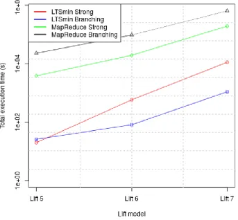
Figure 7.1: LTSmin vs MapReduce for lift models . . . 35
Listing 2.1: Counting of incoming transitions per state. . . 6
Listing 3.1: sequential implementation . . . 8
Listing 3.2: Reading the AUT file (MAP) . . . 11
Listing 3.3: CreateSigs . . . 12
Listing 3.4: CountSigs . . . 12
Listing 3.5: Construct LTS . . . 13
Listing 3.6: Compact LTS . . . 13
Listing 4.1: sequential implementation . . . 16
Listing 4.2: Reading the AUT file (MAP) . . . 19
Listing 4.3: Creating new signatures . . . 20
Listing 4.4: First tau step. . . 21
Listing 4.5: Propagating along tau . . . 22
Listing 4.6: Reconstructing LTS . . . 23
Listing 4.7: Counting signatures . . . 23
Listing 4.8: Constructing the LTS. . . 24
Listing 4.9: Compacting the LTS . . . 24
Table 3.1: Strong bisimulation reduction on the beverage machine . . . 9
Table 4.1: Branching bisimulation on the new beverage machine. . . 17
Table 6.1: Results for the strong bisimulation . . . 29
Table 6.2: Results for the branching bisimulation. . . 31
Chapter 1
Introduction
Today we have the joy of many technological assets. Maybe you are reading this on a laptop, and downloaded this Thesis over the internet. But all these technologies have a drawback; they make life very complex, when you exactly want to know what is happening. Even an ordinary item such as a pencil is very complex due to our modern production processes. It can even be claimed that not a single person on earth has the knowledge and capability to produce a pencil identical to a store-bought pencil.[31] Knowing how the production process of a single pencil works might not be a common thing to question. But what about knowing how the airbags in your car work? How can a consumer, or producer as a matter of fact, know with a 100% certainty that airbags will deploy in case of a crash or will not deploy in case of a rare racing condition in the car computer?
Ironically enough, technology can supply a solution. Within the field of Computer Science a lot of previous and current research is done on model checking[26]. Model checking allows researchers to simulate a process or system, and exhaustively test for wanted or non-wanted properties. Logically, the result of these test are as dependable as your model represents the actual system. The best model then, would be a model representing the system down to its last atom, allowing for every possible interaction with the model. The model of course will become extremely large, a situation known asstate space explosion.
Current research[20, 35, 17] therefore focuses on:
• Storing larger models
• Processing large models faster and smarter
• Reducing the size of models, whilst keeping the same properties
In this thesis we will focus on reducing the size of the models using bisimulation reduc-tion[25, 29]. Bisimulation reduction allows to identify similar states that can be merged whilst preserving certain properties of the model. These similar, or redundant states will be iden-tified by comparing them with other states in the model using a bisimulation relation. The bisimulation relation will identify states showing the same behavior, that therefore can be merged. This process is called bisimulation reduction [25]. A common method to determine the smallest model is using partition refinement[7]. We will elaborate on these techniques is Chapter 2.
The main contributions of this project will be bisimulation reduction with MapReduce. This gives us the following research question:
Research Question: To what extent is MapReduce a suitable platform for bisimulation reduction?
In order to judge the suitability of our solution we will run several tests reducing predetermined models. During these tests we will look at two things that can distinguish our solution opposed to current solutions. Leading to the following subquestions:
Sub-Question 1: How much space does a MapReduce based bisimulation reduction require w.r.t. scaling of the model size?
Sub-Question 2: How much time does a MapReduce based bisimulation reduction require w.r.t. scaling of the model size?
This report is structured as followed: Chapter 2 explains some preliminaries like: What is a model exactly? How can you define bisimulation reduction, and what does Hadoop do? Chapter 3&4 contain two different bisimulation relations with their respectable implemen-tations, more information on their implementation is given in 5. In Chapter 6 we put the implementations to the test, and explain something about the test procedure and the used hardware. After the experiments we will provide the Conclusions and Future work in the final Chapter 7.
1.1
Related work
Chapter 2
Preliminaries
2.1
Model Checking
For the last decade it has become clear that our current society depends more and more on software, often to the point that lives can be at stake when the software does not work correctly. At the same time, software becomes more and more complex, increasing the odds for errors. One way to increase software quality is to use model checking. Using model checking, a model representing for example a piece of software or a protocol is either manually designed or automatically generated using software. This model can then be used to explore whether certain desired properties or undesired properties hold for this model, and thus for the program represented by the model. A way to do model checking is to generate the complete set of states the program can be in when the model of the software is used and to check if one of those states conflicts with predefined rules. Each state in the model represents a unique condition of the software, and the model describes the possible relation between each of these states. The most common problems when model checking are:
• Knowing how to model your system
• State space explosion
State space explosion describes the phenomenon that the amount of states of a model can grow exponentially with the size of the model. State space explosion is a logical result of trying to represent an intricate system by defining all the states a system can be in, e.g. by introducing parallelism.
Bisimulation reduction is a well known technique to reduce this state space [25, 7]. In this thesis we will present a new way to achieve bisimulation reduction using the Hadoop MapRe-duce framework[11]. MapReMapRe-duce is a well-established paradigm in the big data community [16]. Using MapReduce allows for both simple scaling of an algorithm w.r.t. the amount of machines, and migration of the algorithm to another computational cluster. Model checking is a process that is inherently demanding on computing power and memory usage. We think that implementing model checking algorithms using the MapReduce framework can allow users with less computational power to evaluate large models by outsourcing the computing to parties like Amazon EMR [21].
2.2
Labeled Transition Systems
By definition[2], a LTS can be described as a tuple
T S= (S,Act,→, i,AP)
where
• S is the set of states of the system
• Actis the set of actions
• →⊆ S ×Act× S represents the transitions (t−→α swhereα∈Actands, t∈ S)
• i∈ S the initial state of our system
2.2.1
Beverage machines
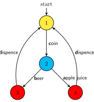
To illustrate matters we will be using some (simplified) models of beverage machines in this thesis. Our beverage machine usually behaves in a predictable manner, one can supply a coin with the actionc(oin), and then select a producta(pple juice)orb(eer). After the selection a τ-step happens in which the machine probably updates its cash registry, and hopefully it will
d(ispence)a cold beverage. The first two versions of this machine can be seen in figure 2.1 and
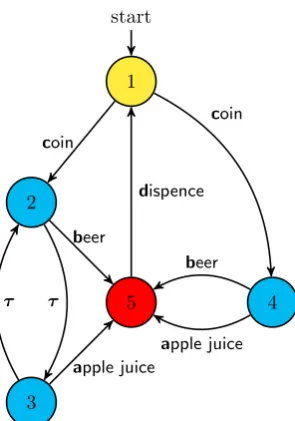
2.2. In chapter 4 we will introduce a more complex beverage machine to illustrate branching bisimulation (figure 4.1).
We now have an idea of what a model and a state space is, and how to describe it. Next, we are going to see if we can make this state space a bit smaller.
2.3
Bisimulation Reduction
To reduce the state space we will try to replace our LTS with a (much) smaller version that has exactly the same behavior as our original LTS. So our new LTS simulates the old LTS and visa versa, or the old LTSbi-simulates the new LTS.
A bisimulation relation Ris a set of states R ⊆ S × S where both states in the relation are said to simulate each other (bisimulation). Intuitively, given (s1, s2) ∈ R, s1 could for
example do all the actions thats2 could do and end up in a similar state as s2. The exact
same goes for the reversed situation. For a formal description of the bisimulation relation we refer to Chapter 3.
If we have two states that can perfectly simulate the other and end up in the same (or a similar) state, we could not distinguish both states. If we replace all these simulating states with one state we have a reduced version of our original LTS. A common way to calculate the reduced LTS, is by using a partitioning algorithm. We will give a short explanation of the idea of the algorithm, more intricate descriptions are given in the respective chapters. The partitioning algorithm states that each state is bi-similar. It then iterates, trying to find states that are in factnot similar, partitioning the state space. The iteration terminates when the algorithm cannot find any non bi-similar states. The termination is guaranteed, since we cannot create more partitions than there are states. At this point the algorithm has found the largest (or coarsest) partitions possible, therefore the result of the algorithm will be the
smallest LTS that is bisimilar to the original LTS. Figure 2.2 shows us the LTS of a beverage
machine, we enabled partition refinement to color all the (strongly) bi-similar states. After reduction, by merging the same colored states we have the original machine shown in 2.1. The formal definition of strong bisimulation can be found in the next chapter.
1 start
2
3 coin
beer apple juice
[image:13.595.86.213.72.264.2]dispence
Figure 2.1: Machine 01
1 start
2
3 4
coin
beer apple juice
[image:13.595.333.496.79.256.2]dispence dispence
Figure 2.2: Machine 02
2.3.1
Signature refinement
The implementations for strong and branching bisimulation that we present in Chapter 3&4 make use of signature refinement. Signature refinement is proposed by Blom and Orzan[8] to allow for more efficient distributed bisimulation reduction. In the algorithm proposed by Kanellakis and Smolka the blocks for each state needs to be calculated and saved in a central table during partitioning[25]. Signature refinement replaces these blocks by defining signatures for each state. States with an equal signature will be assigned to the same partition. The definition for the signature for strong bisimulation is:
sigk(s) ={(α, partk−1(t))|s
α −→t
Where sig0(s) =∅, partk(s) is the current partition for a given state, and k is the current
iteration for the partition refinement. As you can see given a state and its outgoing transitions we can calculate the new signature, and thus partition for this state. In our algorithm we will directly calculate an unique partition number by using a cryptographic hash for the partitions.
partk(s) =hash(sigk(s))
We will lose the option for monotonically increasing partition numbers, but in return all the partitions for a given state can be calculated and assigned solely based on the outgoing transi-tions for that state and without communication between workers. For branching bisimulation a similar approach will be used based on the work by Blom and Pol[9].
2.4
MapReduce
During this project we developed a way to realize partition refinement using the MapReduce framework by Hadoop. Hadoop is a framework initiated by Google to process vast amounts of data[18, 16]. Hadoop offers a framework that handles most of the common tasks needed in distributed implementations, as for example handling the distributed storage of data or errors (e.g. the failure of one of the machines or nodes)[11]. Within the Hadoop-framework there are multiple options for distributed operations, one of these options is the use of distributed algorithms. To develop distributed algorithms, Hadoop has a framework, called MapReduce [16, 38], MapReduce allows easy development of distributed applications. A developer can then easily develop a distributed solution, simply by implementing the MapReduce-framework.
MapReduce requires the developer to divide each distributed algorithm in two steps: the Map and the Reduce-phase. The developer writes a function for the Map-phase that accepts a key-value pair (hk, vi), and outputs another key-value pair (hk0, v0i). In an intermediate step all these key-value pairs are sorted and grouped byk0. Custom sorting algorithms will even allow us to dosecondary sorts on these key-value pairs[34], we will use this in Section 3.3.1. Next, we call the Reducer function with each key and a iteratable with the corresponding values, which we will represent as a list in the pseudo-code (hk0, v0[]i). In some snippets of
pseudo-code it is important to note that we loop multiple times over all the values, since v[]is an iteratable this is technically not possible. This is fixed either by a carefully chosen secondary sort, guarantying the correct order of v[]or by storing the values inv[]locally. MapReduce does not allow for communication or shared variables between reducers and mappers, however MapReduce does offer global counters allowing users to keep track of certain statistics. In our pseudo code counters can be identified by theCOUNTER-prefix. The Reducer-function then uses this data to output a new key-value pair,hk00, v00i. Optionally, the result of this reducer can now be fed to another MapReduce function, or iterate the same MapReduce function. For example, in Listing 2.1 we have a map and reduce function. The goal of the algorithm is to count the total of incoming edges for each state. Given that the map-function is called with s as key and−→a t as value, where s−→a t ∈T S. The map-function than emits (t,1) for each transition, since we want to count the total amount of incoming edges. After grouping ontall these values are send to the reducer. The reducer only has to sum up all the values and emit the amount of incoming edges together with the corresponding state.
input: transition systemhs,(a, t)i
temp:hs,1i
output:hs, count(s)i
5 MAP(k,v)
emit(v.t,1)
REDUCE(k,v[])
emit(k,v.length)
Chapter 3
Strong Bisimulation
We will present a definition for the given Bisimulation relation followed by a regular (naive) algorithm for the sequential case. Then we show the structure of our algorithm in a flow graph, accompanied by the pseudo code for each of the MapReduce-blocks. Ending with a short discussion on the implementation with design choices and encountered difficulties. We will adhere to the same structure for branching bisimulation in chapter 4.
The first bisimulation reduction algorithm we developed is forstrong bisimulation.
3.1
Definition
Strong bisimulation states that two states are bi-similar if, and only if, they can execute the same action and end up in a bi-similar state.
More formally given two transition systems[2]:
T Sδ= (Sδ,Actδ,→δ, iδ), δ= 1,2
The strong bisimulation relationRoverT Sδ is defined asR ⊆ S1× S2
A. (i1, i2)∈ R
B. for all (s1, s2)∈ Rit holds:
1. ifs1
α
−→s01 then there existss2
α
−→s02with (s01, s02)∈ Randα∈Actδ
2. ifs2
α
−→s02 then there existss1
α
−→s01with (s01, s02)∈ Randα∈Actδ
The above definition states that the two initial states in both transition systems need to be bisimilar in condition A. Condition B guarantees that each pair of states (s1, s2) in Ris
actually strongly bisimilar. Meaning thats1 is bisimilar tos2 if and only if each actionαto
a state s0
1 bys1 can be simulated bys2. s2 is not required to make the sameαtransition to
s0
1, but it has to make aα-step to a state that is bisimilar to s01 which can be eithers01 itself
input: transition systemT S= (S,→)
output: table pi, containing the new partitions
reduce()
5 forall states s∈ S dopi[s]:=0end for repeat
// compute signatures
forall states sdosig[s]:=∅ end for forall transitions (s,α,t)∈→do 10 insertSig(s,α,pi[t])end if
end for
// reassign pi according to sig hashtable :=∅
count:=0
15 forall states sdo
if notsig[s] in hashtable.keys()then
hashtable.insert(sig[s],count) inc(count)
end if 20 end for
forall states sdo
pi[s]:= hashtable.lookup(sig[s])
end for untilpi is stable
25
insertSig(t,a,ID)
if not((α,ID)∈sig[t])then
sig[t]:=sig[t]S{(α,ID)}
end if
Listing 3.1: sequential implementation
3.2
Regular algorithm
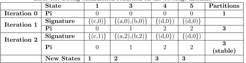
In order to minimize a state space using bisimulation reduction we have to find the largest set (R) of bisimulation relations. A way to do this, is using partition refinement[2, 25]. A simple representation of such an algorithm is given in Listing 3.1. This is a simplified representation of the algorithm proposed by Blom and Orzan[8]. The algorithm works with signatures represented by the variable sig, initially each state has an empty and thus equal signature. States of equal signature will be in equal partitions, these partitions will be stored
in pi. The algorithm iteratively refines these partitions by calculating new signatures, based
on the outgoing transitions for each state. The partition numbers are unique since each new signature is given an unique identifier bycount. The algorithm terminates when the amount of partitions (or unique signatures) stays stable. Termination is guaranteed, because the amount of signatures will increase or stay stable for each iteration, and the total amount of unique signatures can not exceed the total amount of states.
Table 3.1: Strong bisimulation reduction on the beverage machine
State 1 3 4 5 Partitions
Iteration 0 Pi 0 0 0 0 1
Iteration 1 Signature {(c,0)} {(a,0),(b,0)} {(d,0}) {(d,0)}
Pi 0 1 2 2 3
Iteration 2 Signature {(c,1)} {(a,2),(b,2)} {(d,0}) {(d,0})
Pi 0 1 2 2 3
(stable)
New States 1 2 3 3
3.3
MapReduce implementation
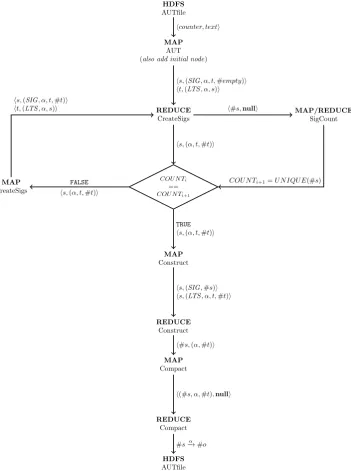
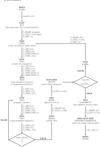
The MapReduce implementation is based on the work by Blom and Orzan[8] and Sch¨atzle et al.[32]. As stated before, the algorithm in listing 3.1 is similar to the algorithm proposed by Blom and Orzan. For our MapReduce implementation we can not make use of a shared table to store the variables sig or pi. For the calculation of the partition table pi a shared table would be an easy solution. In order to be able to do distributed strong bisimulation reduction without a shared hashtable some non-trivial problems need to be solved. In listing 3.1 on line 28 we construct a signature by creating a set of the actions and previous partition for the target state of all the outgoing transitions, creating inductive signatures[9]. On line 15 we use these sets to determine new partitions. Alternatively we could also store this whole set for each state, but this would result in a gigantic blowup of the size of the model. Another way to generate a unique partition number based on the set of states and partition numbers is the use of a cryptographic hash. This guarantees an unique partition number, without communication between workers during the partitioning. A disadvantage of this method is that we lose the fact thatnpartitions will be numbered 0..n−1. The signatures for a given statesare thus generated by hashing the set of all outgoing transitions being: sigk+1=hash({(α, sigk(t))|s−→α t∈→}). An overview of our algorithm is shown in the flowchart in figure 3.1. Each of the steps in the graph are than described in subsection 3.3.2. In the flowgraph thecreateSigs step executes the MapReduce version for the inside of the loop (line 7-23). TheSigCountcounts the signatures, which is needed for the condition on line 24 in the sequential implementation.
3.3.1
Flowchart
In the flowchart in figure 3.1 we have outlined the developed algorithm. Between each Map and Reduce action we have placed the submitted key-value pairs. Often the keys consist of two values, allowing for secondary sorting on the flags supplied with the key. The most important step in the flowchart is theBiSim-step, here we calculate the new signatures for each state. To calculate these signatures the Mapper provides the reducer with the signature of a given state, and all the outgoing transitions for that state. After the generation of the new signatures a separate Map and Reduce function counts the amount of unique signatures inSigCount. If we look at the original algorithm in listing 3.1CreateSigs is similar to the step taken on lines 8-23, where the use ofpi is replaced with a hashing function. CountSigsrepresents the terminating condition on line 24.
HDFS
AUTfile
MAP
AUT (also add initial node)
REDUCE
CreateSigs
COU N Ti
== COU N Ti+1
MAP
CreateSigs
MAP/REDUCE
SigCount
MAP
Construct
REDUCE
Construct
MAP
Compact
REDUCE
Compact
HDFS
AUTfile
hcounter, texti
hs,(SIG, α, t,#empty)i ht,(LTS, α, s)i
hs,(α, t,#t)i
h#s,nulli
hs,(α, t,#t)i
FALSE
TRUE
hs,(α, t,#t)i
hs,(SIG,#s)i hs,(LTS, α, t,#t)i
h#s,(α,#t)i
h(#s, α,#t),nulli
#s−→α #o
hs,(SIG, α, t,#t)i ht,(LTS, α, s)i
[image:18.595.132.484.173.645.2]COU N Ti+1=U N IQU E(#s)
3.3.2
Pseudo code
This section contains pseudo code for the used Mappers and Reducers for the strong bisimu-lation reduction. Each listing starts with the expected input. The intermediary format that is emitted by the Mapper, which will be sorted on both the state and the supplied flag, before it is offered as input to the Reduce function. The output(s) specify the expected out for the reducer which will be offered to another MapReduce task (except for the very last run). Along with each listing an explanation of that step is provided, and the listing will also contain some additional comments.
Loading the model
We read the transitions from an existing state space in the Aldebaran (*.AUT) format[26]. The use of a pre-defined format for allows our tools interoperability with already existing tools. The Aldebaran format consists of a header containing the name of the start state, the amount of states and the number of transitions. Each following line describes a transition, we could state that we simply get supplied the set → from T S. Each transition is emitted with the label ”LTS”, for each state we also emit the signature, which in the initial mapping is the hash for an empty set. The signature for a given stateswill be shorthanded #s.
input: transition system (counterk, textv)// k is not used, v contains a line of text
output: ht,(SIG, α, t,#t)i // for the signature of state t
hs,(LTS, α, t,#t)i // a transition for state s
5
MAP(k,v)
#empty = []
// retrieve the transition from v (s, α, t)←parse text(v)
10 // emit the signature for t emit(t,(SIG, t,#empty)) // emit the transition
emit(s,(LTS, α, t,#empty))
Listing 3.2: Reading the AUT file (MAP)
Creating new signatures
input:hs,(α, t,#t)i // transition as input
temp:hs,(SIG, α, t,#t)i // for the signature of state t ht,(LTS, α, s)i// a transition for state s
output1:hs,(α, t,#t)i // transition with new signature
5 output2:h#s, nulli // signature for counting
MAP(k,v)
// emit the signature for outgoing transitions from s
10 emit(k.s,(SIG, v.t, v.#t))
// emit the reversed transitions
emit(v.t,(LTS, v.α, k.s))
REDUCE(k,v[])
15 new=∅
forvinv[]wherev.type==SIG
// add the outgoing signatures to the new−set new=newS(v.α, v.#t)
// emit the transitions with #new
20 forvinv[]wherev.type==LTS emit1(v.s,(v.α, k.t,hash(new)))
// emit our new signature for counting
emit2(hash(new), null)
Listing 3.3: CreateSigs
Statecount
The emitted signatures from listing 3.3 can now be counted. The output of the map function is sorted and all the duplicate keys are removed. In the reducer we can therefore simply update a global counter, counting the total of discovered states. The algorithm will compare this counter to the old amount of sigs. When the number of signatures is not stable we will continue to the map function in listing 3.3, according to the flowchart in figure 3.1. When the amount of signatures s stabilized we can construct the reduced LTS.
input:h#new, nulli// new signature
temp:h#new, nulli
output:null
5 MAP(k,v)
emit(k, null)
REDUCE(k,v[])
SIG COUNTER.inc();
Listing 3.4: CountSigs
Constructing the reduced LTS
for the destination. The reduce function will than construct #s−→α #tfor each given transition. To remove the duplicate transitions we have the additional task in listing 3.6.
input:hs,(α, t,#t)i // transition
temp:ht,(SIG,#t)i // signature hs,(LTS, α, t,#t)i// transition
output: h#s,(α,#t)i // transition with signatures
5
MAP(k,v)
// emit the signature for t
emit(v.t,(SIG, v.#t))
10 // emit the transition
emit(k.s,(LTS, v.α, v.t, v.#t))
REDUCE(k,v[])
selectvfromv[] wherev.type==SIG
15 #s=v.#t
forvinv[]wherev.type==LTS
emit(#s,(v.α, v.#t))
Listing 3.5: Construct LTS
Output to AUT
Using the sorting function of MapReduce we can remove all duplicate transitions. We auto-matically sort and remove duplicate keys between the mapper and the reducer. The result will be the reduced transition system.
input:h#s,(α,#t)i // transition
temp:h(#s, α,#t), nulli// sort by transition
output: h#s,(α,#t)i // output transition
5
MAP(k,v)
emit((k.#s, v.α, v.#t), null)
REDUCE(k,v[])
10 emit(k,null)
Chapter 4
Branching Bisimulation
4.1
Definition
Branching bisimulation is quite similar, only it preserves the branching structure of the TS better. Internally, the system can take as many unobservable steps (τ-steps) as needed, as long as the observable or visible steps are identical, and when the starting and the end states of theτ-steps are in the bisimulation relation with the same state. We will write the definition by [33] in the style used in Chapter 3. [2, 33] More formally given two transition systems:
T Sδ= (Sδ,Actδ,→δ, iδ), δ= 1,2
The branching bisimulation relationRoverT Sδ is defined asR ⊆ S1× S2
A. (i1, i2)∈ R
B. for all (s1, s2)∈ Rit holds:
1. ifs1
α
−→s01 then there existss2
τ −→∗s00
2
α
−→s0002 −→τ ∗s0 2
with (s1, s002)∈ R ∧(s01, s0002 )∈ R ∧(s01, s02)∈ Rand α∈Actδ\{τ}
2. ifs2
α
−→s02 then there existss1
τ −→∗s00
1
α −→s0001
τ −→∗s0
1
with (s001, s2)∈ R ∧(s0001, s02)∈ R ∧(s01, s02)∈ Rand α∈Actδ\{τ}
3. ifs1
τ
−→s01 then there existss2
τ −→∗s0
2 with (s01, s02)∈ R
4. ifs2
τ
−→s02 then there existss1
τ −→∗s0
1 with (s01, s02)∈ R
The above definition states that the two initial states in both transition systems need to be bisimilar in condition A. Condition B guarantees that each pair of states (s1, s2) in Ris
branching bisimilar. This means thats1 is bisimilar to s2 if and only if each actionα, where
α6=τ, to a states01bys1can be simulated bys2, possibly by first taking an arbitrary amount
of τ-steps, then taking the α-action followed by zero or more τ-steps. The step needs to be simulated, meaning that the transitions need to end in a bisimilar state ((s0
1, s02)∈ R).
If s1 takes a τ-step to s01 then s1 and s2 are bisimilar if and only if s2 also takes zero or
input: transition systemT S= (S,→)
output: table pi, containing the new partitions
reduce()
5 forall states s∈ S dopi[s]:=0end for repeat
// compute signatures
forall states sdosig[s]:=∅ end for forall transitions (s,α,t)∈→do 10 // select all invisible steps
if not(α=τ and pi[s]=pi[t])then insertSig(s,α,pi[t])end if end for
// reassign pi according to sig
15 hashtable :=∅
count:=0
forall states sdo
if notsig[s] in hashtable.keys()then
hashtable.insert(sig[s],count)
20 inc(count)
end if end for
forall states sdo
pi[s]:=hashtable.lookup(sig[s])
25 end for untilpi is stable
insertSig(t,a,ID)
if not((α,ID)∈sig[t])then
30 sig[t]:=sig[t]S{(α,ID)}
forall s∈ S such that s−→τ t and pi[s]=pi[t]do insertSig(s,α,ID)
end for end if
Listing 4.1: sequential implementation
4.2
Regular algorithm
The single threaded algorithm shown in listing 4.1 is the sequential algorithm in the work by Blom and Orzan [7]. For each state a set is created similar as in listing 3.1 but with an additional constraint. This constraint tells us to ignore all states that are invisible, meaning all transitions containing aτ-step where the source and destination are in a shared partition. This set of visible transitions is than propagated back along all invisible τ-transitions. The moment the propagation along the invisible step is finished the signature for each state is created based on these (propagated) sets.
1 start
5 2
3
4 coin
dispence
coin
beer
apple juice τ
τ
apple juice
[image:25.595.214.362.69.280.2]beer
Figure 4.1: Machine 03
4.3
MapReduce implementation
For our MapReduce implementation we needed a more elaborate scheme, allowing for the nested loops in the original algorithm. The outer loop is similar to the original loop in the strong bisimulation implementation. More specifically lines 7-13 correspond to theLabel-step in the flowgraph. The inner loop provides the propagation along the invisible transitions. In the sequential implementation this happens on lines 30-32. Figure 4.2 shows this more intricate scheme. The propagation step of the algorithm requires us to keep a set of all the states (Σs), opposed to only passing a hash (#s) of the set.
Table 4.1: Branching bisimulation on the new beverage machine
State 1 2 3 4 5 Partitions
Iteration 0 Pi 0 0 0 0 0 1
Iteration 1
Signature {(c,0)} {(b,0)} {(a,0)} {(a,0),(b,0}) {(d,0)}
Traversed - {(a,0),(b,0}) {(a,0),(b,0}) -
-Pi 0 1 1 1 2 3
Iteration 2
Signature {(c,1)} {(b,2)} {(a,2)} {(a,2),(b,2}) {(d,0)}
Traversed - {(a,2),(b,2}) {(a,2),(b,2}) -
-Pi 0 1 1 1 2 3
[image:25.595.83.569.657.773.2]4.3.1
Flowchart
HDFS
AUTfile
MAP
AUT
(add initial node and reversed transition)
RED
LABEL
(create set based on visible states)
MAP
TAU1 (prepare for propagation)
RED
TAU2 (map signatures of parents to propagating transitions)
MAP
TAU2 (propagate signature)
RED
TAU2
(count propagated signatures)
N EW COU N T
== 0
MAP
BUILD (rebuild LTS)
RED
BUILD (flip from and to)
MAP/RED
COUNT (count unique signatures)
COU N Ti
==
COU N Ti+1
MAP
LABEL
MAP
CONSTRUCT (pass signature for from state)
RED/MAP/RED
CONSTRUCT&REDUCE (build and compact reduced LTS)
HDFS
AUTfile hcounter, texti
ht,(HASH,#empty)i hs,(LTS, a, t,#empty)i ht,(REV, s)i
hs,(SIG,Σs)i hs,(BRA, a, t)i hs,(FWD PASS, t)i hr,(PAR, s,Σs)i
hs,(SIG,Σs)i hs,(BRA, a, t)i hs,(PAR, t,Σt)i hs,(FWD PASS, t)i ht,(BWD PASS, s)i
hs,(SIG,Σs)i hs,(BRA, a, t)i hr,(PRE, s,Σs)i
hs,(SIG,Σs)i hs,(BRA, a, t)i hs,(PRE, t,Σt)i ht,(BWD PASS, s)i
hs,(BRA, a, t)i hs,(SIG,Σs)i hr,(PRE, s,Σs)i
hs,(HASH,Σs)i ht,(LTS, a, s,#0)i hs,(LTS, a, t,#s)i
FALSE
TRUE
hs,(HASH,#s)i hs,(LTS, a, t,#t)i
h(#s, a,#t),()i
FALSE
TRUE
[image:26.595.131.477.79.590.2]ht,(HASH,#t)i hs,(LTS, a, t,#t)i ht,(REV, s)i
4.3.2
Pseudo code
Reading from AUT file
A difference with branching simulation is that we have to pass the reversed transition to be able to propagate the signature we are going to create along theinvisible steps.
input: transition systemcounterk, textv)// we only use v, which contains our text
output: ht,(HASH,#empty)i // pass the signature for state t
hs,(LTS, a, t,#empty)i // pass the transition
ht,(REV, s)i // pass the reversed transition
5
MAP(k,v)
#empty = []
// retrieve the transition from v (s, α, t)←parse text(v)
10 // pass hash of the state emit(t,(HASH,#empty)) // pass the transition
emit(s,(LTS, a, t,#empty))
// pass reverse transitions for later use
15 emit(t,(REV, s))
Creating new signatures
We split up our LTS in the visible and invisible part. The invisible and visible part we respectively output with the typeFWD PASS and BRA. We use all the visible transitions for a given state to create the set sigset. This set we emit for this state and also coupled to all the incoming transitions.
input:hs,(LTS, α, t,#t)i // the transition
temp:hs,(HASH,#s)i // pass the hash hs,(LTS, a, t,#t)i // pass the transition
ht,(REV, s)i // pass the reversed transition
5 output:hs,(SIG,Σs)i // the signature set for s
hs,(BRA, a, t)i // the visible transition
hs,(FWD PASS, t)i // the invisible transition hr,(PAR, s,Σs)i // the reversed transitions
10 MAP(k,v)
// pass hash of the state
emit(t,(HASH,#t)) // pass the transition
emit(s,(LTS, a, t,#t))
15 // pass reverse transitions for later use emit(t,(REV, s))
REDUCE(k,v[])
// get the signature for the current state
20 selectv∈v[] wherev.type==HASH
fromsig = v.#s
// emit the invisible transitions
forv∈v[]where v.type==LTS ∧
(v.a==τ∧f romsig==v.#t)
25 emit(s,(FWD PASS, t))
// calculate the signatureset
forv∈v[]where v.type==LTS ∧
not (v.a==τ∧f romsig==v.#t) sigset = sigsetS(v.a, v.#t)
30 // emit the signatureset for this state emit(k.s,(SIG, sigset))
// emit the visible transitions
forv∈v[]where v.type==LTS ∧
not (v.a==τ∧f romsig==v.#t)
35 emit(k.s,(BRA, v.a, v.t))
// emit the reversed transitions with the signatureset for propagation purposes
forv∈v[]wherev.type==REV
emit(v.r,(PAR, k.s, sigset))
First tau step
The firstτ-step looks up the passed back signatures inPARfor all the transitions inFWD PASS. We add all the new signatures to this state and pass this new set to all the propagating invisible transitions. We count all the new signatures that are added in a global counter.
input:hs,(SIG,Σs)i // signatureset for s
hs,(BRA, a, t)i // visible transition
hs,(FWD PASS, t)i // invisible transition
hr,(PAR, s,Σs)i // reversed transition for propagation
5 temp:hs,(SIG,Σs)i // signatureset for s
hs,(BRA, a, t)i // visible transition
hs,(PAR, t,Σt)i // invisible transition for propagation hs,(FWD PASS, t)i // invisible transition
hs,(BWD PASS, r)i // reversed invisible transition
10 output: hs,(SIG,Σs)i // signatureset for s
hs,(BRA, a, t)i // visible transition
hr,(PRE, s,Σs)i // invisible transition
MAP(k,v)
15 // emit the invisible transitions reversed
if (v.type==FWD PASS)
emit(v.t,(BWD PASS, k.s)) // pass through
emit(k,v)
20
REDUCE(k,v) sigs =∅ newsigs =∅
// pass the visible transitions
25 forv∈v[] wherev.type==BRA emit(k,v)
// get the signatureset for s
selectv∈v[]wherev.type==SIG sigs =v.Σs
30 // get all the invisible transitions
forv∈v[] where v.type==FWD PASS
// get the signatureset from the reversed transitions
forw∈v[]where v.type==PAR∧v.t == w.t newsigs = newsigsS(w.Σt)
35 // emit how much new signatures we found
SIG COUNTER.inc(|newsigs\sigs|);
// add the new signatureset to the signatureset sigs = sigsS
newsigs // emit our new signatureset
40 emit(s,(SIG, sigs))
// emit our invisible transitions with the signatureset
forv∈v[] wherev.type==BWD PASS
emit(v.r,(PRE, k.s, sigset))
Propagating along tau steps
The map-function copies the invisible sets for the propagation toBWD PASS. In the reducer we emit the visible states. We calculate the propagating signatures and pass these for the current state, and also coupled to the invisible transitions for propagation. This step will be repeated until no more changes in the signatures occur.
input:hs,(SIG,Σs)i // signatureset for s
hs,(BRA, a, t)i // visible transition
hs,(PRE, t,Σt)i // invisible transition
temp:hs,(SIG,Σs)i // signatureset for s
5 hs,(BRA, a, t)i // visible transition
hs,(PRE, t,Σt)i // invisible transition
hs,(BWD PASS, r)i // reversed invisible transition for propagation
output:hs,(SIG,Σs)i // signatureset for s
hs,(BRA, a, t)i // visible transition
10 hr,(PRE, s,Σs)i // invisible transition
MAP(k,v)
forv∈v[]wherev.type==PRE
emit(v.t,(BWD PASS, k.s))
15 emit(k,v)
REDUCE(k,v) sigs =∅ newsigs =∅
20 // pass the visible transitions forv∈v[]wherev.type==BRA
emit(k,v)
// get the signatureset for s
selectv∈v[] wherev.type==SIG
25 sigs =v.Σs
// get all the invisible transitions
forv∈v[]where v.type==PRE newsigs = newsigsS(w.Σt)
// emit how much new signatures we found
30 SIG COUNTER.inc(|newsigs\sigs|);
// add the new signatureset to the signatureset sigs = sigsS newsigs
// emit our new signatureset
emit(s,(SIG, sigs))
35 // emit our invisible transitions with the signatureset forv∈v[]wherev.type==BWD PASS
emit(v.r,(PRE, k.s, sigset))
Reconstructing LTS
Based on the set of signatures for a given set we create a hash. This hash is emitted for the state. Both the visible and the invisible transitions are emitted with the to-state as key. The reducer retrieves the hash for a given state s. This hash is then added to all the transitions, and the to- and from-states are flipped to recreate the original transitions with the new signatures added.
input:hs,(SIG,Σs)i // signatureset for s
hs,(BRA, a, t)i // visible transition
hs,(PRE, t,Σt)i // invisible transition
temp:hs,(HASH,#s)i // hash for s
5 hs,(LTS, a, r,#empty)i // transitions for s
output: hr,(LTS, a, s,#s)i // transitions for s
MAP(k,v)
sigset =∅
10 // get the signatureset for s selectv∈v[]wherev.type==SIG
sigset =v.Σs
// create a new signature for s and emit it
emit(s,(HASH,hash(sigset)))
15 // emit all visible transitions reversed forv∈v[] wherev.type==PRE
emit(v.t,(LTS, v.a, k.s,#empty)) // emit all invisible transitions reversed
forv∈v[] wherev.type==BRA
20 emit(v.t,(LTS, τ, k.s,#empty))
REDUCE(k,v)
// get the signature for s
selectv∈v[]wherev.type==HASH
25 sig = v.\#s
// add the signature to the transitions and un−reverse them
forv∈v[] wherev.type==LTS
emit(v.r,(LTS, v.a, k.s, sig))
Listing 4.6: Reconstructing LTS
Counting signatures
We emit all the signatures and after sorting we can simply count all the unique signatures.
input:hs,(LTS, a, t,#t)i// transitions
temp:h(#s),) // signature for s
output: null
5 MAP(k,v)
// emit the signature
emit((#t),)
REDUCE(k,v[])
10 // count the signatures
SIG COUNTER.inc()
Constructing the LTS
To construct the new LTS is similar to the construction for the strong bisimulation: we need to convert the original LTS consisting of the triples s−→α t to a minimized LTS according to the partitions. We can achieve that by substituting the partition numbers creating the set of triples #s−→α #t. For a given transition the map function will pass the signature for that state, and all the outgoing transitions, already containing the signature for the destination. The reduce function will then construct #s−→α #tfor each given transition.
input:hs,(LTS, a, t,#t)i // transition for s
temp:hs,(HASH,#s)i // signature for s hs,(LTS, a, t,#t)i// transitions for s
output:h(#s, a,#t),()i // transition for s
5
MAP(k,v)
forv∈v[]
// emit the transition
emit(k,v)
10 // emit the signature for t emit(t,(HASH,#t))
REDUCE(k,v)
// retrieve the hash for
15 selectv∈v[] wherev.type==HASH
sig = v.\#s // emit the transitions
forv∈v[]wherev.type==LTS
emit((sig, v.a, v.#t),())
Listing 4.8: Constructing the LTS
Compacting the LTS
For the compacting we can leverage MapReduce to output a list without duplicate transitions.
input:h(#s, a,#t),()i// transition for s
temp:h(#s, a,#t),()i// transition for s
output:h(#s, a,#t),()i// transition for s
5 MAP(k,v)
emit(k,null)
REDUCE(k,v[])
emit(k,null)
Chapter 5
Implementation & Optimization
We would like to elaborate a bit on the more technical details of the code of both the algorithms. The code as shown in the pseudo code above, along with the flow graphs should give an impression on how to implement bisimulation reduction with MapReduce. However the actual implementation in Java with the MapReduce framework is a bit more elaborate.
5.1
Implementation
5.1.1
File format
Reading the model requires us to have the model in a format that is readable using the MapReduce framework. A common and simple way to read files in MapReduce is to retrieve data from a text file. Therefore we have chosen to first format our models in the Aldebaran format. Between each iteration however it is not recommended to use a text based file format. Hadoop offers the use of sequence files. The sequence files can contain the key value pairs in a binary format, which saves a lot of space. For the signature counting in the strong bisimulation we have chosen a separate approach. To reduce the bandwidth used for the counting we output a separate file containing only the signatures during the signature creation. In a small scale experiment we experienced a minor speed-up of up to 2x for large models.
5.1.2
Signatures
The signatures themselves needed to have a few properties. First of all, the signatures need to be relatively small, we achieved that by using a hashing function. However, we want to be sure we do not have any hash collisions. A hash collision could mean that two states suddenly could have a similar signature when they are not supposed to have that. An easy way to make sure that collisions are virtually impossible is to use a cryptographic hash. The cryptographic hash we chose (SHA-256) has such low chances on a hash collision, that we are safe to assume that it will never happen. A quick calculation, assuming that SHA-256 is a proper hashing algorithm, learns that based on the birthday problem[3] we can approximate the chancepon a collision givennsignatures to be:
p≈1
2
n
2128
2
Meaning that when we have significantly less states than 2128 we can safely ignore collisions. The disadvantage of using a cryptographic hash is that they are often designed to be slow in order to prevent attacks on e.g. hashed passwords[28]. We decided that SHA-256 is still reasonably fast with the advantage that we can be sure that we will not have hash collisions.
5.1.3
Technicalities
and grouper. We have written this partitioner in such a way that all key value pairs with the same state in the key will be offered to the same reducer. However, the keys will be sorted based on the type of the key-value pair. This way we can ensure that the values will always arrive in a predetermined order. Otherwise we could for example not retrieve the signature of a key before we attach it to later transitions as can be seen in listing 3.3.
If you look at listing 4.3 you can see that we output the key value pair ({P AR, r},{s,Σs}). The Σs however is quite a large variable. It basically is a set containing pairs with a label and a byte array. To make sure that our value is correctly written to disk by Hadoop required research in the data structures in Hadoop that allow this.
5.2
Potential Optimizations
Designing the branching bisimulation algorithm we thought about some worst case scenarios. A possible scenario is that we might get very long invisible tau steps, which requires a lot of iterations. Observing that iterations are quite expensive with our algorithm, we tried to devise a solution. Our proposed solution was to try and cut some of these long tau steps in pieces. We decided to focus at states that have both visible and invisible outgoing transitions. By simply ignoring all the invisible steps for these states we could stop the propagation of long tau steps. Our conjecture was, that in subsequent iterations these signatures would still propagate and thus the branching bisimulation would still be correct. However this suspicion proved wrong. As a counter example we will take the beverage machine from figure 4.1. When we would ignore the silent steps in state 2 and 3 they would be split up after the first iteration. This is a coarser partition than what should be allowed, because state 2,3&4 belong to the same partition. Therefore we will not further pursue this option.
Discussing the previous optimization, another possible optimization came up. It would of course be allowed to make our partition less coarse, if done the correct way. A possibility is to not use all the possible labels in the calculation of a signature. As long as our last (and stabilizing) refinement does use all the labels. While propagating along the silent steps we could keep track which labels are still propagating. Labels that take a long time to propagate could be ignored for that round. In later rounds the long tau chains responsible for this behavior might been broken up and allow for a faster propagation off the labels.
A different approach is to use the transitive closure for all the (non-branching) tau-steps. This would prevent the massive amount of inner iterations, since all the signatures propagate at once. The time-complexity for n states isO(log(n)). However, in the worst case the required space could be up to O(n2) [24]. We have done a small scale experiment and calculated the
Chapter 6
Experiments
We have benchmarked both of our algorithms. To run the models we needed a cluster of several computers to run this on. Luckily we were in the position to make use of the CTIT-cluster of the University of Twente. We have benchmarked both the strong and branching bisimulation algorithms on a set of models. This set of models describes several protocols and models suited for benchmarking. The size of the models varied from small to very large. The smallest model only has 289 states and 1224 transitions. The largest model available has 7.041.674.929 states, this is already beyond the maximal value of an unsigned 32 bit integer which can be maximal 232−1 (4.294.967.295).
6.1
Experimental setup
For our setup we have used the cluster of CTIT. This cluster consists of 44 nodes for the calcula-tion of our MapReduce tasks. The nodes each have a single Opteron 4386 processor and 64GB of memory. Our main program runs on a central node, from where it offers the MapReduce tasks for processing by the cluster. This main program also logs our benchmark information. We keep track of information relevant about the model like the amount of signatures after each iteration. We also keep track of the time spend for each iteration.
6.1.1
Models
Our models are part of the VLTS-benchmark[14]. The state space is converted using LTSmin[10] to the Aldebaran format. The Aldebaran format is very suitable to read with MapReduce since it is a plain text file containing each transition on a separate line. For the larger models this is a serious drawback, since the files will get too large for storing as a simple text file. Since for larger models we can therefore not use the Aldebaran format we looked at other formats offered by LTSmin. We eventually decided on using the ”.dir” format, which is an uncom-pressed variant of the Generic Container Format used by LTSmin[10]. We have developed a separate program that can load these uncompressed state spaces and convert them directly to the sequence file format we already use internally in our algorithm. We have added the lift 7-model, which is similar to cwi 2165 8723 (lift 5) and cwi 33949 165318 (lift 6), except for the size of the model. This allows us for easy comparison on the scaling of the algorithm with respect to the state space. The VLTS-benchmark also includes vasy 40 60, a model that has a state space specifically designed to require a lot of transitions with 20002 transitions for strong bisimulation reduction. The full information on all the models can be found in table 8.1.
6.1.2
Results
partition is found. This can be easily shown by defining a LTS where there exist two labels,
a and b. Initially all the states belong to one single partition. Now we could merge all the duplicate transitions we would have a lot ofa-transitions going from this single partition to this same partition. It is easy to see that without knowing the final (coarsest) partitioning we might merge a lot of transitions that in the final LTS should be separate transitions. The similar calculation times per iteration therefore tells us that the main time spend in each iteration is corresponding to the amount of transitions of our original model. An advantage of this is that with a single execution of the algorithm we still can have a statistically fair estimation of the execution time for each transition, by taking the average of the time spend for each iteration of a given model. In the tables below you can see the average execution time for a iteration on a given model, together with the standard deviation over this set. The small deviation tells us that data-throughput is the main bottleneck for our implementation, and we thus have a fair approximation. Taking the average for the MapReduce part of the algorithm also has another advantage. Since the cluster is shared with other users the scheduler may schedule some other tasks for other users in between our execution. In the averaging the incidental interleaving for other tasks is therefore ignored.
6.2
Strong bisimulation
We ran our bisimulation algorithm for the whole suite, increasing the size of the model for each run. In table 6.1 the results for these runs can be viewed. Each row starts with the model name and the amount of states for the given model, we than have the averaged time for each ”BiSim”-action (see figure 3.1). The column ”Sig” contains the time used for each signature counting. The last three columns show the total amount of iterations used for the calculation, the cumulative time for the reduction of the model, and the amount of states in the reduced model.
6.2.1
Results
When we look at our table we can see that the time spent in signature counting takes slightly less time than the signature creation. However, the time needed per iteration does scale with the amount of initial transitions. We can explain the difference by looking at the amount of data that is transferred for the signature calculation opposed to the signature counting. For the signature counting we read and write for each transition a single signature in the mapping phase. The reducer only counts the amount of signatures. The signature creation for each transition we read and write the whole transition, and all the incoming transitions for that transition. We can conclude that we have to transfer more than twice the amount of data.
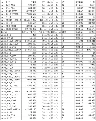
We now want to have a more detailed look at how our algorithm scales. In order to create a clear picture we have decided to plot the initial amount of transitions against the time spendper iteration. We have chosen for the initial amount of transitions because it is a clear indicator of the model size. Since the total time spend on calculation increases with the amount of iterations needed for the reduction we can not do a fair comparison between the models. Therefore a clearer indication of scalability is the time needed per iteration. Figure 6.1 shows this in two figures. The first figure shows us all the models on a logarithmic scale for both axis allowing for the larger models to fit within the frame. The second figure shows us the models with less than 108transitions.
6.2.2
Conclusion
From the figures we can see that up to 10 million transitions the execution time per iteration is not increasing exponentially. We can also see that the minimum time per iteration is around 30 seconds, probably this has to do with the startup costs for each MapReduce phase. Above 107 transitions the amount of transitions per second we process seems to be increasing. Our
second figure shows a close-up for all the models with less than 108transitions. We indeed see
model name transitions BiSim Sig Iterations Time Reduced
cwi_1_2 2387 27±3s 24±4s 27 0:23:35 1132
cwi_142_925 925.429 34±5s 22±3s 16 0:15:41 3410
cwi_214_684 684.419 26±1s 22±0s 86 1:08:02 77.292
cwi_2165_8723 8.723.465 34±1s 23±0s 66 1:03:57 31.906
cwi_2416_17605 17.605.592 44±3s 23±1s 42 0:49:35 95.610
cwi_3_14 14.552 24±1s 21±0s 61 0:45:33 62
cwi_33949_165318 165.318.222 176±21s 33±2s 91 5:23:22 122.035
cwi_371_641 641.565 26±1s 23±1s 73 0:59:25 33.994
cwi_566_3984 3.984.157 28±1s 23±0s 16 0:15:04 15.518
cwi_7838_59101 59.101.007 101±11s 26±1s 94 3:23:45 966.470
lift7 2.875.174.785 1751±472s 102±15s 120 53:29:21 441.015
vasy_0_1 1224 24±0s 21±0s 5 0:03:48 9
vasy_10_56 56.156 24±1s 21±0s 33 0:24:46 2112
vasy_11026_24660 24.660.513 59±4s 29±2s 50 1:15:24 882.341
vasy_1112_5290 5.290.860 33±0s 28±3s 4 0:05:10 265
vasy_116_368 368.569 25±1s 22±1s 29 0:22:43 116.456
vasy_12323_27667 27.667.803 62±7s 30±2s 35 0:55:59 996.774
vasy_1_4 4464 23±1s 21±0s 7 0:05:11 28
vasy_157_297 297.000 25±1s 22±0s 27 0:21:12 4289
vasy_164_1619 1.619.204 26±1s 22±2s 6 0:05:19 1136
vasy_166_651 651.168 25±1s 22±1s 10 0:08:01 83.436
vasy_18_73 73.043 24±1s 21±0s 22 0:16:26 4087
vasy_25_25 25.216 24±0s 21±0s 2 0:01:32 25.217
vasy_2581_11442 11.442.382 38±2s 23±0s 21 0:22:58 2.581.374
vasy_386_1171 1.171.872 26±1s 22±1s 8 0:06:48 113
vasy_4220_13944 13.944.372 39±2s 25±1s 39 0:43:25 1.356.477
vasy_4338_15666 15.666.588 42±2s 23±0s 21 0:24:22 2.581.374
vasy_52_318 318.126 26±1s 21±0s 15 0:11:44 8142
vasy_574_13561 13.561.040 42±3s 23±0s 5 0:06:54 3577
vasy_5_9 9676 23±0s 21±1s 5 0:03:45 145
vasy_6020_19353 19.353.474 49±4s 26±8s 9 0:13:36 7168
vasy_6120_11031 11.031.292 37±2s 25±1s 21 0:23:29 5199
vasy_65_2621 2.621.480 28±1s 22±1s 4 0:03:54 65.536
vasy_66_1302 1.302.664 25±1s 21±0s 4 0:03:25 66.929
vasy_69_520 520.633 25±0s 22±1s 12 0:09:27 69.754
vasy_720_390 390.999 26±0s 21±1s 5 0:04:00 3292
vasy_8082_42933 42.933.110 73±8s 25±1s 10 0:18:05 408
vasy_8_24 24.411 23±1s 21±1s 14 0:10:25 416
vasy_83_325 325.584 25±1s 21±1s 10 0:07:50 83.436
[image:37.595.83.484.80.582.2]vasy_8_38 38.424 24±1s 21±1s 5 0:03:48 219
Table 6.1: Results for the strong bisimulation
6.3
Branching bisimulation
(a) Logarithmic plot (b) Linear plot (under 108)
Figure 6.1: Iteration-times vs state space for Strong bisimulation
6.3.1
Results
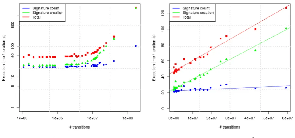
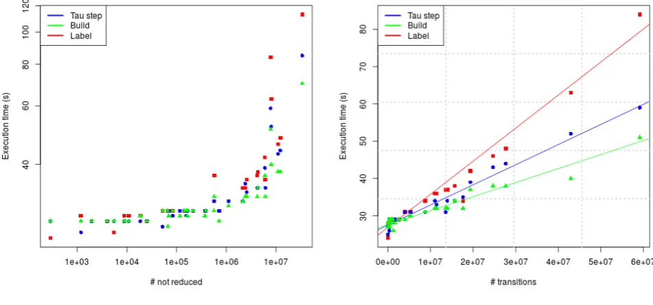
When we look at our table we can see result quite similar to that shown for strong bisimulation. In general the ”label”-step takes the most time, this is when the signature sets are created and a lot of tuples are passed. During the ”tau”-steps we have a large signature set that slowly grows. This set is not trivially small, so we infer that the time spent is in part because of the traversal of and read/write-operations on this large set. The ”build”-step has to read this large signature set, but only has to write one hash for each set, which might explain the quicker iterations by the ”build”-step. Overall time is significantly higher than the strong bisimulation implementation, which is not surprising given the addition of several tau-steps. Using tables 6.1,6.2 and 8.1 we can focus on few models that have zeroτ-transitions. In theory given the absence ofτ-transitions, the strong and branching implementation should give the same result. Moreover, since the branching implementation always executes one (unnecessary) τ-step we should expect the branching implementation to take twice as long as the strong implemen-tation. If we look at models vasy 0 1, vasy 1112 5290,vasy 25 25,vasy 574 13561, and
vasy 65 2621we can indeed see that there is a factor 2 between the total execution time for branching and strong bisimulation for these models.
6.3.2
Conclusion
From the figures we can see that for branching bisimulation up to 1 million transitions the execution time per iteration a linear fit can be made. We can also see that the minimum time per iteration is still around 30 seconds. Since this was also the case with the strong bisimulation reduction we are strengthened in our conjecture this has to do with the startup costs for each MapReduce Job. Above 106 transitions the amount of transitions per second we process seems to be increasing. Our second figure shows a close-up for all the models with less than 107 transitions. We indeed see a linear increase in this lower region.
6.4
Additional experiments
model name transitions calc tau build Iterations (tau) Time Reduced
cwi_1_2 2387 27±2s 27±2s 27±2s 8(128) 1:07:38 67
cwi_142_925 925.429 29±1s 29±2s 29±2s 6(30) 0:22:58 23
cwi_214_684 684.419 29±2s 29±2s 29±1s 18(840) 7:00:02 478
cwi_2165_8723 8.723.465 34±2s 31±2s 31±3s 14(696) 6:20:39 4256
cwi_2416_17605 17.605.592 34±0s 35±3s 32±2s 2(51) 0:34:22 730
cwi_3_14 14.552 27±0s 27±2s 27±0s 2(122) 0:57:08 2
cwi_33949_165318 165.318.222 113±3s 85±5s 70±3s 16(1080) 26:39:44 12.463
cwi_371_641 641.565 29±1s 29±2s 28±2s 6(195) 1:40:50 2134
cwi_566_3984 3.984.157 31±0s 31±2s 29±2s 6(33) 0:26:41 198
cwi_7838_59101 59.101.007 84±5s 59±3s 51±3s 46(2016) 35:06:43 62.031
vasy_0_1 1224 24±2s 27±0s 27±0s 5(5) 0:08:58 9
vasy_10_56 56.156 28±2s 27±2s 27±3s 33(42) 1:02:34 2112
vasy_11026_24660 24.660.513 46±2s 43±2s 38±2s 44(201) 3:52:30 775.618
vasy_1112_5290 5.290.860 31±3s 31±2s 30±2s 4(4) 0:09:14 265
vasy_116_368 368.569 29±2s 29±2s 28±2s 17(406) 3:31:49 22.398
vasy_12323_27667 27.667.803 48±2s 44±2s 38±2s 31(149) 2:53:32 876.944
vasy_1_4 4464 28±0s 25±3s 27±0s 2(2) 0:03:38 4
vasy_157_297 297.000 29±3s 28±3s 29±1s 21(63) 0:58:04 3038
vasy_164_1619 1.619.204 29±1s 29±2s 28±2s 5(7) 0:10:41 992
vasy_166_651 651.168 29±4s 29±2s 29±2s 6(18) 0:16:43 42.195
vasy_18_73 73.043 28±3s 27±2s 28±2s 14(81) 0:54:48 2326
vasy_25_25 25.216 27±0s 27±0s 27±0s 2(2) 0:03:42 25.217
vasy_2581_11442 11.442.382 36±2s 33±2s 32±2s 14(56) 0:53:17 704.737
vasy_386_1171 1.171.872 29±1s 29±1s 29±0s 5(20) 0:16:57 71
vasy_4220_13944 13.944.372 37±3s 34±2s 32±2s 27(124) 1:54:49 1.186.266
vasy_4338_15666 15.666.588 38±1s 34±2s 34±2s 14(56) 0:57:11 704.737
vasy_52_318 318.126 29±0s 26±3s 29±2s 4(11) 0:10:33 66
vasy_574_13561 13.561.040 37±3s 31±2s 32±2s 5(5) 0:12:19 3577
vasy_5_9 9676 25±4s 27±2s 27±0s 5(10) 0:11:13 112
vasy_6020_19353 19.353.474 42±0s 39±3s 37±0s 2(12) 0:12:51 256
vasy_6120_11031 11.031.292 36±1s 34±2s 32±3s 16(64) 1:03:25 2505
vasy_65_2621 2.621.480 29±2s 29±0s 29±0s 4(4) 0:08:25 65.536
vasy_66_1302 1.302.664 29±0s 29±2s 26±2s 3(7) 0:07:47 51.128
vasy_69_520 520.633 29±2s 29±2s 28±3s 12(24) 0:27:25 69.753
vasy_720_390 390.999 29±3s 29±4s 27±3s 5(5) 0:08:45 3292
vasy_8082_42933 42.933.110 63±1s 52±2s 40±2s 6(18) 0:30:21 290
vasy_8_24 24.411 27±2s 27±1s 27±0s 10(62) 0:41:29 170
vasy_83_325 325.584 29±1s 28±3s 29±2s 6(18) 0:16:43 42.195
[image:39.595.88.491.73.538.2]vasy_8_38 38.424 28±2s 27±2s 27±0s 5(5) 0:08:56 193
Table 6.2: Results for the branching bisimulation
both the implementations took respectively 129 and 140 seconds for the first iteration (where the model is loaded). We attribute the lack of difference between the two implementations to the fact that both files are not offered in a split form to Hadoop, but instead are both a single big file.
We have ran a small benchmark on the speedup for using smaller key-value pairs in the signature counting for the strong bisimulation. As stated in subsection 5.1.1 the use of smaller key-value pairs led to a maximum 2x-speedup.
(a) Logerithmic plot (b) Linear plot (under 107)
Chapter 7
Conclusion and Future Work
7.1
Conclusion
In Chapter 3 we introduced an algorithm for strong bisimulation reduction using MapReduce. The algorithm is based on the work by Blom and Orzan. We have studied the distributed strategy used by Blom and Orzan and created an algorithm without the need for central tables. We have introduced the use of cryptographic hashes for the calculation of partitions to circumvent the lack of communication between workers. In Chapter 4 we have introduced Branching bisimulation and created an additional algorithm to allow Branching bisimulation with MapReduce. The differences in complexity of these implementations can be seen when comparing figure 3.1 and 4.2. The resulting algorithms were benchmarked on the CTIT cluster using the VLTS-benchmark set[14]. The resulting reduced models validated in both cases against models that are reduced with the existing toolset LTSmin[26]. From all the metrics we have compiled two tables (tabel 6.1&6.2) and created two graphs showing the scaling of time versus the state space (figure 6.1&6.2).
During our experiments we saw that the execution-time for a MapReduce job takes a relatively long time. We have estimated that there is a startup cost for each job of circa 30 seconds. This means that the reduction of transition systems that need a lot of iterations can be very high. Extreme cases such as the vasy 40 60 which take over 20.000 iterations therefore could not be benchmarked within an acceptable time-frame. Each iteration all of our data is passed over the disk. Therefore it is not unreasonable to see a factor 10-100 slow down compared to a mpi-based implementation (e.g. LTSmin). From our experiments we have concluded that the separate iteration times of our algorithm scale linearly up to 108 transitions for strong bisimulation and 107 for branching bisimulation. On larger models the iteration time increases exponentially, therefore we where not able to benchmark our largest model (lift8).
7.2
Comparison with existing tools
We have taken the MapReduce benchmark for thelift5,lift6andlift7-model and compared it with the execution time for the existing distributed implementation in LTSmin. The results are shown in figure 7.1. Note that the vertical axis is logarithmic. Here we can clearly see the price of the (slow) iteration in MapReduce, showing a factor 100 between the MapReduce implementation and an existing state-of-the-art tool. Based on this graph our conjecture is that our MapReduce implementation will not be a viable alternative for existing tools, given our current framework.
7.3
Hadoop and MapReduce as a Programming Paradigm
for Model Checking
MapReduce are not a suitable platform for high-iterative tasks, even with solutions optimized for iterative tasks[36]. Since a lot of model checking algorithms have an iterative nature[2] these are not suited for MapReduce. Bisimulation reduction (e.g. strong, branching, weak) is a great example. But also algorithms using least fix point or greatest fix point calculations, such as Computational Tree Logic (CTL) or Linear Temporal Logic (LTL)[2]. A model checking tech-nique that is a possibility is the exploration of large state spaces. However, creation of large state spaces that will not fit on a researchers machine have limited value, since we concluded that bisimulation reduction or full fledged checkers using LTL or CTL is not feasible using MapReduce. However, by severely restricting oneself, it could be possible to check properties written in First Order Logic[2] that do not require large amounts of iterations.
We conclude that MapReduce could be a valuable paradigm for model checking tools, given that:
• The overhead per iteration is very low.
• Map-tasks are able to merge input streams, allowing us to temporally ”park” data.
• Additionally central data structures are allowed to prevent large data-throughputs.