New Developments in Teaching Electromagnetics through Advanced Numerical Simulations and Virtual Experiments

(1)

ISSN Online: 2151-4771 ISSN Print: 2151-4755

DOI: 10.4236/ce.2018.916216 Dec. 27, 2018 2878 Creative Education

New Developments in Teaching

Electromagnetics through Advanced Numerical

Simulations and Virtual Experiments

Wuliang Yin

1,2

, Qian Zhao

3

, Kai Zhang

3

, Zhigang Qu

1*

1_{College of Electronic Information and Automation, Tianjin University of Science and Technology, Tianjin, China} 2_{Sensing, Imaging and Signal Processing, School of EEE, University of Manchester, Manchester, UK}

3_{School of Engineering, Qufu Normal University, Rizhao, China}

Abstract

Electromagnetic field is an advanced topic which requires thinking in abstract terms and with imagination. This paper presents authors’ experience in teaching electromagnetics at Tianjin University, China and demonstrates that this difficult subject can be tackled with the help of advanced numerical simulations and virtual experiments. Commercial simulation packages and in house developed software such as the Finite Elements Method (FEM), the Boundary Element Method (BEM) and an analytical method were used for this purpose. Overall, students have provided positive feedback for this teaching methodology.

Keywords

Electromagnetic Course, Numerical Simulations, Virtual Experiments

1. Introduction

There is a widespread opinion among students that electromagnetics is tradi-tionally a difficult subject to teach as it involves abstract and unfamiliar concepts such as fields and waves especially for students coming from a circuit back-ground and there were little available teaching materials in the subject of

elec-tromagnetic fields for measurements (Ulaby & Hauck, 2000; Warnick et al.,

1997). The spectacular growth of computer simulation in electromagnetic analy-sis and design over the last several decades has been considered as a unique op-portunity for reversing such a situation. Different tools and experiences have

been reported (de Magistris, 2005). Nevertheless, the author states that, the

sys-How to cite this paper: Yin, W. L., Zhao, Q., Zhang, K., & Qu, Z. G. (2018). New Developments in Teaching Electromagnet-ics through Advanced Numerical

Simula-tions and Virtual Experiments. Creative

Education, 9, 2878-2883.

https://doi.org/10.4236/ce.2018.916216

Received: October 9, 2018 Accepted: December 24, 2018 Published: December 27, 2018

http://creativecommons.org/licenses/by/4.0/

(2)

DOI: 10.4236/ce.2018.916216 2879 Creative Education

tematic use of numerical simulations and virtual experiments in teaching elec-tromagnetics is still not commonplace.

Since 2008, a course has been developed in Tianjin University which targeted undergraduate students in the major of electronic instrumentation and meas-urements, who needs knowledge in electromagnetics in a context of measure-ment. This paper developed a computer aided approach which exploits the ad-vances in computing and graphics in recent years to make the electromagnetic fields something concrete to visualise and hence enhancing the teaching and learning process in this subject.

The aim is to help the student develop a physical understanding of funda-mental concepts and principles of EM and to help the student understand the dynamic character of EM fields, the three-dimensional nature of waves in gen-eral as well as to motivate and challenge the student to analyze measurement re-sults and to try to explain unexpected rere-sults.

This approach has been trialled at the undergraduate level and the learning outcome suggested that most 2nd and 3rd year students managed to master the subject to a satisfactory level. After the classes, the students are able to design and build a “real” hardware system that incorporated many of the EM concepts and principles they learned, as well as material they learned from other courses.

2. Customized Software—Formulation and Numerical Results

In order to delve into the detailed process of the solutions, customised software which can be fully accessed is needed. Three typical methods have been tried—the Finite Elements Method (FEM), the Boundary Element Method (BEM) and an analytical methods. In all cases, all codes were developed in MATLAB.

2.1. The Analytical Method and Its Numerical Results

In the analytical method, a simple electrostatic problem is illustrated as shown in

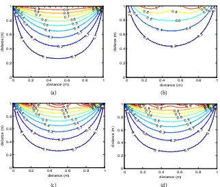
Figure 1 where the letter n means the number of terms (Binns et al., 1992). As can be seen, each term has a particular spatial frequency inherent to it and therefore the number of terms is a deciding factor in reaching an accurate solu-tion. When the number of the term is less than 3, the solution shows spatial fea-tures on the top boundary, which are artefacts. Satisfactory solution is achieved when the number of the turns reaches 15.

2.2. The Finite Elements Method and Its Numerical Results

The finite element method is a numerical method that is used to solve boun-dary-value problems characterized by a partial differential equation and a set of boundary conditions. The geometrical domain is discretized using sub-domain elements, called the finite elements. A set of shape functions is used to represent the primary unknown variable in the each element and several linear equations will be obtained. A global matrix system is formed after the assembly of all

(3)

(a) (b)

[image:3.595.213.535.66.339.2]

(c) (d)

Figure 1. The equipotential lines field distribution when (a) n = 15; (b) n = 1; (c) n = 2; (d) n = 3.

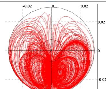
In the Finite Elements Method, a 2D flow meter equation is solved here as an

example. The flow meter equation is (Jin, 2014;Yin & Peyton, 2010; Tonti, 2001)

( )

[

]

2

_σ

_V _{· (}

_{σ υ}

₎

∇ = ∇ ×B (1)

where the left side is a Laplace operator and the right side is the EMF caused by the Faraday effect. This equation can be solved by the Finite Elements Method

and could be depicted as shown in Figure 2.

2.3. The Boundary Element Method and Its Numerical Results

The boundary element method (BEM) is a well established numerical technique in the engineering community, The BEM has been successfully applied to solve

many problems in different kinds of areas (Portela et al., 1992).

In the Boundary Element Method, a PEC case is used to elucidate the scat-tered field when a perfectly electrical conductive (PEC) object is placed in a

pri-mary pressed magnetic field, as shown in Figure 3.

3. Commercial Software Simulated Results

COMSOL and ANSOFT are two packages widely used for EM simulations. An

inductive problem was simulated and its results are presented in Figure 4 and

Figure 5 (Yin, et al., 2011).

4. Conclusions

The development of new teaching materials for an electromagnetics course with 01 0.₁ 0.1 0.1 0.1 0.1 0.₂ 0.2 0.2 0.2 0.2 0.3 0.3 0.3 0.3 0.4 0.4 0.4 0.4 0.5 0.5 0.5 0.5 0.6 0.6 0.6 0.6

0.7 _0.7 0.7

0.8 _0.8 0.8

0.9 0.9 0.9

1 1 1 1 1 1 1 1 1 1 1 1 1 1 1 1

distance (m) di st anc e ( m )

0 0.2 0.4 0.6 0.8 1

0 0.2 0.4 0.6 0.8 1 0.₂ 0.2 0.2 0.2 0.2 0.4 0.4 0.4 0.4 0.6 _0.6 0.6

0.8 1 0.8 10.8

distance (m) di st anc e ( m )

0 0.2 0.4 0.6 0.8 1

0 0.2 0.4 0.6 0.8 1 0. 1 0.₁ 0.1 0.1 0.1 0.1 0. 2 0.2 0.2 0.2 0.2 0.3 0.3 0.3 0.3 0.4 0.4 0.4 0.4 0.5 0.5 0.5 0.5

0.6 _0.6 0.6

0.7

0.810.9 _0.810.9 0.90.81

1.1 1.1 distance (m) di st anc e ( m )

0 0.2 0.4 0.6 0.8 1

0 0.2 0.4 0.6 0.8 1 _0. 1 0.₁ 0.1 0.1 0.1 0.1 0. 2 0.2 0.2 0.2 0.2 0.3 0.3 0.3 0.3 0.4 0.4 0.4 0.4 0.5 0.5 0.5 0.5

0.6 _0.6 0.6

0.7 _0.7 0.7

0.8 _0.8 0.8

0.9 _0.9 0.9 0.9

1 1 1 1

1.1 1.1 distance (m) di st anc e ( m )

0 0.2 0.4 0.6 0.8 1

(4)

[image:4.595.211.538.68.205.2] [image:4.595.291.457.238.352.2]

[image:4.595.283.468.384.539.2]

Figure 2. Current flow patterns for a uniform B field from different directions.

[image:4.595.271.475.573.706.2]

Figure 3. The scattered field due to a crack in a uniformed electromagnetic field.

Figure 4. Magnetic flux distributions from a a coil at the bottom.

Figure 5. Eddy current distributions due to a coil in the front.

0 5 10 15 20 25

0 10 20 30 40 50

0 5 10 15 20 25

mm

(5)

a targeted cohort of undergraduate students in the major of electronic instru-mentation and measurements has been presented in this paper. With the aid of advanced numerical simulations and virtual experiments, it is proved that the

subject electromagnetic field can be successfully delivered to 2nd_{and 3}rd_year

students with no previous background in this subject. Commercial simulation packages and in house developed software such as the Finite Elements Method (FEM), the Boundary Element Method (BEM) and an analytical method were used for this purpose. Positive feedback from students has provided evidence for the merit of this teaching methodology.

Feedback from the students of the EM courses has been very favorable, even though most students invariably complain about the amount of time it takes to do simulation exercises. The most important thing is that the students seem to appreciate EM rather than avoid it, and in fact they demonstrated overall posi-tive attitude towards the course for both the lectures and the lab.

Conflicts of Interest

The authors declare no conflicts of interest regarding the publication of this pa-per.

References

Binns, K. J., Lawrenson, P. J., & Trowbridge, C. W. (1992). The Analytical and Numerical Solution of Electric and Magnetic Fields. Chichester: Wiley.

de Magistris, M. (2005). A MATLAB-Based Virtual Laboratory for Teaching Introductory Quasi-Stationary Electromagnetics. IEEE Transactions on Education, 48, 81-88.

https://doi.org/10.1109/TE.2004.832872

Jin, J. (2014). The Finite Element Method in Electromagnetics (3rd ed.). Hoboken, NJ: Wiley.

Polycarpou, A. C. (2006). Introduction to the Finite Element Method in Electromagnet-ics. Synthesis Lectures on Computational Electromagnetics, 1, 1-126.

https://doi.org/10.2200/S00019ED1V01Y200604CEM004

Portela, A., Aliabadi, M. H., & Rooke, D. P. (1992). The Dual Boundary Element Method: Effective Implementation for Crack Problems. International Journal for Numerical Methods in Engineering, 33, 1269-1287.

https://doi.org/10.1002/nme.1620330611

Tonti, E. (2001). Finite Formulation of the Electromagnetic Field. Progress in

Electro-magnetics Research, 32, 1-44. https://doi.org/10.2528/PIER00080101

Ulaby, F. T., & Hauck, B. L. (2000). Undergraduate Electromagnetics Laboratory: An In-valuable Part of the Learning Process. Proceedings of the IEEE, 88, 55-62.

https://doi.org/10.1109/5.811601

Warnick, K. F., Selfridge, R. H., & Arnold, D. V. (1997). Teaching Electromagnetic Field Theory Using Differential Forms. IEEE Transactions on Education, 40, 53-68.

https://doi.org/10.1109/13.554670

Yin, W., & Peyton, A. J. (2010). Sensitivity Formulation Including Velocity Effects for Electromagnetic Induction Systems. IEEE Transactions on Magnetics, 46, 1172-1176.

(6)

Yin, W., Chen, G., Chen, L., & Wang, B. (2011). The Design of a Digital Magnetic Induc-tion Tomography (MIT) System for Metallic Object Imaging Based on Half Cycle De-modulation. IEEE Sensors Journal, 11, 2233-2240.