Differential Evolution Using Opposite Point for Global Numerical Optimization

(1)

Differential Evolution Using Opposite Point for Global

Numerical Optimization

Youyun Ao1_{, Hongqin Chi}2

1_{School of Computer and Information, Anqing Teachers College, Anqing, China;}2_{College of Information, Mechanical and Electrical}

Engineering, Shanghai Normal University, Shanghai, China. Email: youyun_ao@tom.com

Received September 25th_{, 2010; revised May 8}th_{, 2011; accepted May 20}th_{, 2011}

ABSTRACT

The Differential Evolution (DE) algorithm is arguably one of the most powerful stochastic optimization algorithms, which has been widely applied in various fields. Global numerical optimization is a very important and extremely difficult task in optimization domain, and it is also a great need for many practical applications. This paper proposes an opposition-based DE algorithm for global numerical optimization, which is called GNO2DE. In GNO2DE, firstly, the opposite point method is employed to utilize the existing search space to improve the convergence speed. Secondly, two candidate DE strategies “DE/rand/1/bin” and “DE/current to best/2/bin” are randomly chosen to make the most of their respective advantages to enhance the search ability. In order to reduce the number of control parameters, this algorithm uses an adaptive crossover rate dynamically tuned during the evolutionary process. Finally, it is validated on a set of benchmark test functions for global numerical optimization. Compared with several existing algorithms, the performance of GNO2DE is superior to or not worse than that of these algorithms in terms of final accuracy, convergence speed, and robustness. In addition, we also especially compare the opposition-based DE algorithm with the DE algorithm without using the opposite point method, and the DE algorithm using “DE/rand/1/bin” or “DE/current to best/2/bin”, respectively.

Keywords: Differential Evolution; Evolutionary Algorithm; Global Numerical Optimization; Stochastic Optimization

1. Introduction

Global numerical optimization problems arise in almost every field such as industry and engineering design, applied and social science, and statistics and business, etc. The aim of global numerical optimization is to find global optima of a generic objective function. In this paper, we are most interested in the following global numerical minimization problem [1,2]:

 





min f x , L x U (1)

where f x

 

is the objective function to be minimized,



x x1, , ,2 xn



Rn

  

x is the real-parameter variable

vector, L



l l1, , ,2  ln



is the lower bound of the vari-

ables and U



u u1, , ,2  un



is the upper bound of the

variables, respectively, such that xi



l ui, i



.

Many real-world global numerical optimization problems have many objective functions that are non-differ- entiable, non-continuous, non-linear, noisy, flat, random, or that have many local minima, multiple dimensions, etc. However, the major challenge of the global numerical optimization is that the problems to be optimized have many local optima and multiple dimensions. Such prob-

lems are extremely difficult to be optimized and find reliable global optima [3,4]. Therefore, increasing require- ments for solving global numerical optimization in various application domains have encouraged many research- ers to find a reliable global numerical optimization algorithm. However, in the last decades, this problem remains intractable, theoretically at least [5].

(2)

come the limitations of traditional global numerical optimization methods, mainly in terms of unknown system parameters, multiple local minima, non-differentiability, or multiple dimensions, etc. [5,11].

Lately, some new methods for global numerical optimization were gradually introduced. Particle Swarm Op- timization (PSO) was originally proposed by J. Kennedy as a simulation of social behavior, and it was initially introduced as an optimization method in 1995 [12]. PSO has been a member of the wide category of Swarm Intel- ligence methods for solving global numerical optimization problems [13-15]. Differential Evolution (DE) was introduced by Storn and Price in 1995, and developed to optimize real-parameter functions [3,16,17]. DE mainly uses the distance and direction information from the current population to guide its further search, and it mainly has three advantages: 1) finding the true global minimum regardless of the initial parameter values; 2) fast convergence; 3) using a few control parameters. In addition, DE is simple, fast, easy to use, very easily adaptable and useful for optimizing multimodal search spaces [18-22]. Re- cently, DE has been shown to produce superior performance, and perform better than GA and PSO over some global numerical optimization problems [13,14]. There- fore, DE is very promising in solving global numerical optimization problems.

This paper proposes an opposition-based DE algorithm for global numerical optimization (GNO2DE). This algorithm employs the opposite point method to utilize the existing search spaces to speed the convergence [21-24]. Usually, different problems require different settings for the control parameters. Generally, adaptation is introduced into an evolutionary algorithm, which can improve the ability to solve a general class of problems, without user interaction. In order to improve the adaptation and reduce the control parameter, GNO2DE uses a dynamic mechanism to dynamically tune the crossover rate CR during the evolutionary process. Moreover, GNO2DE can enhance the search ability by randomly selecting a candidate from strategies “DE/rand/1/bin” and “DE/current to best/2/bin”. Numerical experiments clearly show that GNO2DE is feasible and effective.

The remainder of this paper is organized as follows. Section 2 briefly introduces the basic idea of the DE algorithm. Section 3 describes in detail the proposed GNO2DE algorithm. Section 4 presents the experimental setup adopted and provides an analysis of the experimental results obtained from our empirical study. Finally, our conclusions and some possible paths for the future research are provided in Section 5.

2. The Classical DE Algorithm

The DE algorithm is a population-based stochastic opti-

mization algorithm like many evolutionary algorithms such as genetic algorithms using three similar genetic operators: crossover, mutation, and selection [7]. The main difference in generating better solutions is that genetic algorithms mainly rely on crossover while DE mainly relies on mutation operation. The DE algorithm uses mutation operation as a search mechanism and selection operation to direct the search toward the prospective re- gions in the search space. The DE algorithm also uses a non-uniform crossover that can take child vector parameters from one parent more often than it does from oth-ers. By using the components of the existing population members to generate trial vectors, the recombination (i.e., crossover) operator efficiently shuffles information about successful combinations, enabling the search for a better solution space [3,16,17].

A global numerical optimization problem consisting of n parameters can be represented by a n-dimensional vec- tor. In DE, a population of NP solution vectors is ran-

domly created at the start, where NP4. The popula-

tion is successfully improved by applying mutation, crossover, and selection operators [13,25,26].

2.1. Randomly Initializing Population

Like other many evolutionary algorithms, the DE algorithm starts with an initial population, which is randomly generated when no preliminary knowledge about the solution is available. In DE, let us assume that an individual xi G, 



xi,1,G,xi,2,G, , xi n G, ,



stands for the thi individual of population PG (population size NP) at the generation G. The population P₀



x_1,0,x_2,0, , x_NP_,0



is initialized as





, ,0

, : _{i j} _j _j _j _j

i NP j n x l rand u l

        (2)

where NP is the population size, n is the number of variables, rand_j is a uniformly distributed random number in the range [0,1], and x_{i j}_{, ,0} is the jth variable of

the thi individual at the initial generation, which is initialized within the jth range _l u_j, _j_.

2.2. Mutation Operation

In the mutation phase, DE randomly selects three distinct individuals from the current population. For each target vector x_{i G}_, , the thi mutant vector is generated based on the three selected individuals as follows:





1 2 3

, 1 , , ,

i G  r G F r G r G

v x x x (3)

where i1, 2, , NP, random indexes

1, ,2 3 {1, 2, , }

r r r   NP are randomly chosen integers, mu-

(3)

factor F is a control parameter of the DE algorithm,

which controls the amplification of the differential varia-tion (xr G₂, xr G₃, ). And the scaling factor F is a real constant factor in the range [0, 2] and is often set to 0.5 in the real applications [27].

The above strategy is called “DE/rand/1/bin”, it is not the only variant of DE mutation which has been proven to be useful for real-valued optimization. In order to classify the variants of DE mutation, the notation:

DE x y z is introduced where 1) x specifies the

vector to be mutated which currently can be “rand” (a randomly chosen population vector) or “best” (the vector of lowest cost from the current population); 2) y is the

number of difference vectors used; 3) z denotes the

crossover scheme, there are two crossover schemes often used, namely, “bin” (i.e., the binomial recombination) and “exp” (i.e., the exponential recombination). Usually, there are the following several differential DE schemes often used in the global optimization [3]:

“DE/best/1/bin”:



1 2



, 1 , ,

i G  best F r G r G

v x x x (4)

“DE/current to best/2/bin”:







1 2



, 1 , , ,

i G  i F best i G  F r G r G

v x x x x x (5)

“DE/best/2/bin”:



1 2





3 4



, 1 , ,

i G  best F r G r G  F r  r

v x x x x x (6)

“DE/rand/2/bin”:









1 2 3 4 5

, 1

i G  r  F r  r  F r  r

v x x x x x (7)

where xbest is the best individual of the current population G. The scaling factor F is the control parameter

of the DE algorithm.

2.3. Crossover Operation

In order to increase the diversity of the perturbed parameter vectors, the crossover operator is introduced. The new individual is generated by recombining the original vector xi G, 



xi,1,G,xi,2,G, , xi n G, ,



and the mutant vector vi G, 1



vi,1,G1,vi,2,G1,...,vi n G, , 1



according to the following formula:



 



, , 1

, , ,

if [0,1] [1, ]

, otherwise i j G

i j G

i j G v

w rand CR j rand n

x     _      (8)

where rand[0,1] stands for a uniformly distributed random number in the range [0,1], and rand[1, ]n is a randomly chosen index from the set {1, 2, , } n to ensure that at least one of the variables should be changed and

, 1 i G

w does not directly duplicate xi G, . And the

cross-over rate CR is a real constant in the range [0,1], one of control parameters of the DE algorithm. After crossover, if one or more of the variables in the new solution are outside their boundaries, the following repair rule is ap-plied [25]:









, , 1 , , 1

, , 1 , , 1 , , 1

, , 1

1

, if 2

1

, if 2

, otherwise

i j G j i j G j

i j G j i j G j i j G j i j G

w l w l

w l w u w u

w              _        (9)

2.4. Selection Operation

After mutation and crossover, the selection operation selects to decide that the new individual wi G, 1 or the original individual xi G, will survive to be a member of the next generation. If the fitness value of the new individual wi G, 1 is better than that of the original one xi G, then the new individual wi G, 1 is to be an offspring in the next generation (G + 1) else the new individual

, 1 i G

w is discarded and the original one xi G, is retained in the next generation. For a minimization problem, we can use the following selection rule:



  

, 1 , 1 ,

, 1 ,

, if ,

, otherwise.

i G i G i G

i G i G f f         

w w x

x

x (10)

where f

 

 is the fitness function, and xi G, 1 is the offspring of xi G, in the next generation (G + 1).

2.5. The General Framework of the DE Algorithm

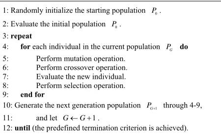
The above operations (i.e., mutation, crossover, and selection) are repeated NP (population size) times to generate the next population of the current population. These successive generations are generated until the predefined termination criterion is satisfied. The main steps of the DE algorithm are given in Figure 1.

1: Randomly initialize the starting population P₀. 2: Evaluate the initial population P₀.

3: repeat

4: for each individual in the current population PG do 5: Perform mutation operation.

6: Perform crossover operation. 7: Evaluate the new individual. 8: Perform selection operation. 9: end for

10: Generate the next generation population PG1 through 4-9,

11: and let G G 1.

[image:3.595.310.535.577.714.2]

(4)

3. The Proposed GNO2DE Algorithm

Similar to all population-based optimization algorithms, two main steps are distinguishable for the DE, population initialization and producing new generations by evolutionary operations such as selection, crossover, and mutation. GNO2DE enhances these two steps using the opposite point method. The opposite point method has been proven to be an effective method to evolutionary algorithms for solving global numerical problems. When evaluating a point to a given problem, simultaneously computing its opposite point can provide another chance for finding a point closer to the global optimum. The concept of the opposite point is defined as follows [21- 24]:

Definition 1 Let us assume that xi G, is the thi point of the population PG (population size NP) at the generation G in the n-dimensional space. The opposite point oi G, 



oi,1,G,oi,2,G, , oi n G, ,



is completely defined by its components as follows:

, , , ,

i j G j j i j G

o  l u x (11) where i1, 2, , NP , j1, 2, , n , l_j and uj are the lower and the upper limits of the variable xi j G, , , respectively.

3.1. Generating the Initial Population Using the Opposite Point Method

Generally, population-based Evolutionary Algorithms randomly generate the initial population within the boundaries of parameter variables. In order to improve the quality of the initial population, we can obtain fitter starting candidate solutions by utilizing opposite points, even when there is no a priori knowledge about the solution (s). The procedure of generating the initial population using the opposite point method is given as follows:

Step 1: Randomly initialize the starting population P0 (population size NP).

Step 2: Calculate the opposite population of P0 using the opposite point method, and obtain the opposite population OP0.

Step 3: Select theNPfittest individuals from P0OP0 as the initial population P0.

3.2. Evolving the Population Using the Opposite Point Method

By applying a similar approach to the current population, the evolutionary process can be forced to jump to a new solution candidate, which may be fitter than the current one. After generating new population by selection, crossover, and mutation, the opposite population is calculated

and the NP fittest individuals are selected from the

union of the current population and the opposite popula-

tion. Following steps describe the procedure:

Step 1: The offspring population PG1 of the current population PG is generated after performing the corresponding successive DE operations (i.e., mutation, crossover, and selection).

Step 2: Calculate the opposite population of PG1 using the opposite point method, and obtain the opposite population OPG1.

Step 3: Select the NP fittest individuals from

1 1

G G

P OP as the next generation population PG1.

Step 4: Let G G 1.

3.3. Adaptive Crossover Rate CR

In DE, the aim of crossover is to improve the diversity of

the population, and there is a control parameter CR

(i.e., the crossover rate) to control the diversity. The smaller diversity is easy to result in the premature convergence, while the larger diversity reduces the convergence speed. In conventional DE, the crossover rate CR is a constant value in the range [0,1]. Inspired by non- uniform mutation, this paper introduces an adaptive crossover rate CR, which is defined as follows [28]:

1

b t CR r

T

 _{ } 

  _ _{ } _  

  (12)

where r is a uniform random number from [0,1], t

and T are the current generation number and the maxi-

mal generation number, respectively. The parameter b

is a shape parameter determining the degree of depen- dency on the iteration number and usually is set to 2 or 3. In this study, b is set to 3.

The property of CR causes the crossover operator to

search the solution space uniformly initially when t is

small, while to search the solution space very locally when t is large. This strategy increases the probability

of generating a new number close to its successor than a random choice. Therefore, at the early stage, GNO2DE uses a bigger crossover rate CR to search the solution

space to preserve the diversity of solutions and prevent premature convergence; at the later stage, GNO2DE employs a smaller crossover rate CR to search the solu-

tion space to enhance the local search and prevent the fitter solutions found from being destroyed. The relation of generation vs crossover rate CR is plotted in Figure 2.

3.4. Adaptive Mutation Strategies

(5)

[image:5.595.60.284.86.265.2]

Figure 2. The graph for generation vs crossover rate CR.

cooperative advantages, GNO2DE randomly chooses a mutation scheme from two candidates “DE/rand/1/bin” (i.e., Equation (3)) and “DE/current to best/2/bin” (i.e., Equation (5)), and the new mutant vector v_{i G}_, _₁ is gen-

erated according to the following formula [27]:

, 1

Equation (3), if [0,1] 0.5

Equation (5), otherwise i G rand      

v (13)

where rand[0,1] is a uniform random number from the

range [0,1].

3.5. Approaching of Boundaries

In the given optimization problem, it has to be ensured that some boundary values are not outside their limits. Several possibilities exist for this task: 1) The positions that beyond the boundaries are newly generated until the positions within the boundaries are satisfied; 2) the boundary-exceeding values are replaced by random num- bers in the feasible region; 3) The boundary is appro- ached asymptotically by setting the boundary-offending value to the middle between old position and boundary [29]:









, , 1 , , 1

, , 1 , , 1 , , 1

, , 1

1 _{, if} 2

1

, if 2

, otherwise

j i j G i j G j

i j G i j G j i j G j i j G

l w w l

w w u w u

w              _       (14)

After crossover, if one or more of the variables in the new vector wi G, 1 are outside their boundaries, the violated variable value wi j G, , 1 is either reflected back from the violated boundary or set to the corresponding boundary value using the repair rule as follows [30]:

















































, , 1 , , 1

, , 1

, , 1 , , 1

, , 1

, , 1 , , 1

, , 1

1 _{, if} _{1 3}

2

, if 1 3 2 3

2 , if 2 3 1

,if 1 3 2

, if 1 3 2 3

2 ,

j i j G i j G j

j i j G j

j i j G i j G j

i j G

i j G j i j G j

j i j G j

j i j G

l w p w l

l p w l

l w p w l

w

w u p w u

u p w u

u w                                 

 if



p 2 3





wi j G_{, ,} ₁ uj



                (15)

where p is a probability and a uniformly distributed

random number in the range [0,1].

3.6. The Framework of the GNO2DE Algorithm

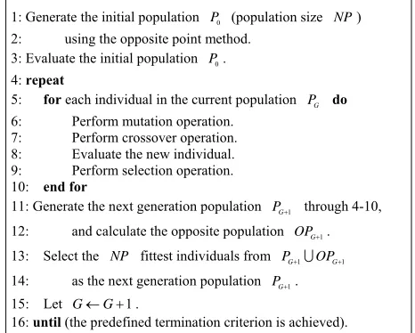
DE creates new candidate solutions by combining the parent individual and several other individuals of the same population. A candidate replaces the parent only if it has better fitness value. The initial population is selected randomly in a uniform manner between the lower and upper bounds defined for each variable. These bounds are specified by the user according to the nature of the problem. After initialization, DE performs mutation, crossover, selection etc., in an evolution process. The general framework of the GNO2DE algorithm is described in Figure 3.

4. Numerical Experiments

4.1. Benchmark Functions

In order to test the robustness and effectiveness of GNO2DE, we use a well-known test set of 23 benchmark functions [1,2,31-33]. This relatively large set is neces- sary in order to reduce biases in evaluating algorithms.

1: Generate the initial population P₀ (population size NP) 2: using the opposite point method.

3: Evaluate the initial population P₀. 4: repeat

5: for each individual in the current population PG do 6: Perform mutation operation.

7: Perform crossover operation. 8: Evaluate the new individual. 9: Perform selection operation. 10: end for

11: Generate the next generation population PG1 through 4-10,

12: and calculate the opposite population OPG1.

13: Select the NP fittest individuals from PG1OPG1

14: as the next generation population PG1.

15: Let G G 1.

[image:5.595.306.539.528.715.2]

16: until (the predefined termination criterion is achieved).

(6)

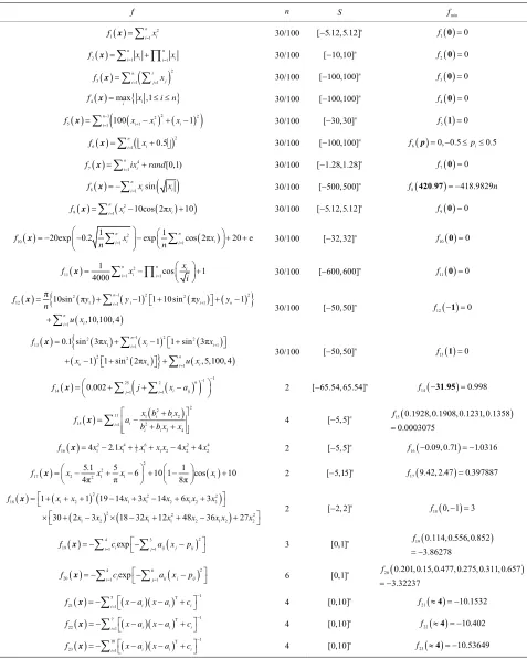
The complete description of all these functions and the corresponding parameters involved are described in Ta-

[image:6.595.58.535.139.736.2]

ble 1 and APPENDX. These functions can be divided into three different categories with different complexities:

Table 1. The 23 benchmark test functions f1- f23.

f n S fmin

  2

1 1

n i i

f x 



_x 30/100 [ 5.12,5.12]_ n  

1 0

f 0   

2 1 1

n n

i i

f x 



 x 



 x 30/100 [ 10,10]

n

 f2 0 0

 





2

3 1 1

n i

j

i j

f x 

 

_ _x 30/100 [ 100,100] n  

3 0

f 0 

 





4 max_i i,1

f x  x  i n 30/100 [ 100,100] n  

4 0

f 0 

  1



2



2  2



5 1 100 1 1

n

i i i

i

f x 



 x x  x 30/100 [ 30,30] n

 f5 1 0

 





2

6 1 0.5

n i i

f x 



_ _x _ 30/100 [ 100,100] n  

6 0, 0.5 i 0.5 f p   p

  4

7 1 [0,1)

n i i

f x 



_ix rand 30/100 [ 1.28,1.28] n  

7 0

f 0 

 

8 1 sin

n

i i

i

f x  



_x x 30/100 [ 500,500]_ n  

8 . 418.9829

f 420 97   n

 



2  



9 1 10cos 2π 10

n

i i

i

f x 



 x  x  30/100 [ 5.12,5.12]

n

 f9 0 0

  2  

10 1 1

1 1

20exp 0.2 n exp n cos 2π 20 e

i i

f x x

n  n 

  _ _

  _



_ _



_ 

x 30/100 [ 32,32] n  

10 0

f 0 

  2

11 1 1

1 cos 1 4000 n n _i i i i x f x i       _ _  





x 30/100 [ 600,600] n  

11 0

f 0 

 



       



 

1 2 2

2 2

12 1 1 1

1

π _10sin _π ₁ _{1 10sin} _π ₁

,10,100, 4 n

i i n

i n

i i

f y y y y

n u x        _  _  



x

30/100 [ 50,50] n  

12 0

f  1

 



     

   



 

1 2

2 2

13 1 1 1

2 2

1

0.1 sin 3π 1 1 sin 3π

1 1 sin 2π ,5,100, 4 n

i i

i

n

n n i i

f x x x

x x u x

       _  _   _  _ 



x

30/100 [ 50,50]_ n  

13 0

f 1 

  ₂₅



₂





₆



-1 1 14 0.002 j1 i1 i ij

f j x a



 

 

_ 







 _

x 2 [ 65.54,65.54] n  

14 . 0.998

f 31 95 

 





2 2

11 1 2

15 1 2

3 4

i i

x b b x

f a

b b x x        _ _     



x 4 [ 5,5]_ n 150.1928, 0.1908, 0.1231,0.1358

0.0003075 f



  2 4 1 6 2 4

3

16 41 2.11 1 1 2 4 2 4 2

f x  x  x  x x x  x  x 2 [ 5,5]_ n   16 0.09, 0.71 1.0316

f   

  2 2  

17 2 2 1 1 1

5.1 5 ₆ _{10 1} 1 _cos ₁₀ 4π π 8π

f _x  x  x  _  _  _ x 

   

x 2 [ 5,15] n  

17 9.42, 2.47 0.397887

f 

   





 





2 2 2

18 1 2 1 1 2 1 2 2

2 2 2

1 2 1 1 2 1 2 2

1 1 19 14 3 14 6 3

30 2 3 18 32 12 48 36 27

f x x x x x x x x

x x x x x x x x

 

 _        _

 

_         _

x

2 [ 2, 2] n  

18 0, 1 3

f  

  4 3





2

19 i1 iexp j1 ij j ij

f x  



_c _



_a x p _ 3 [0,1]n 190.114,0.556, 0.852

3.86278 f

 

  4 6





2

20 i1 iexp j1 ij j ij

f x  



_c _



_a x p _ 6 [0,1]n 200.201,0.15,0.477,0.275,0.311,0.657

3.32237 f

 

  5   T 1

21 i1 i i i

f x a x a c

  

 



_    _

x 4 [0,10]n  

21 10.1532

f 4  

  ₇   _T 1

22 i1 i i i

f x a x a c

  

 



_    _

x 4 [0,10]n   22 10.402

f 4  

  ₁₀   _T 1

23 i1 i i i

f x a x a c

  

 



_    _

x 4 [0,10]n  

23 10.53649

f 4  

(7)

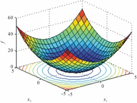
1) unimodal functions ( f1 - f7), which are relatively easy to be optimized, but the difficulty increases as the

di-mensions of the problems increase (see Figure 4); 2)

multimodal functions (f8 - f13), which have many local minima, represent the most difficult class of problems for many optimization algorithms (see Figure 5); 3) multimodal functions ( f14 - f23), which contain only few local optima (see Figure 6). It is interesting to note that some functions have unique features: f6 is a discontinuous step function having a single optimum; f7 is a noisy function involving a uniformly distributed random variable within the range [0,1]. In unimodal functions the convergence rate is our main interest, as the optimization is not a hard problem. Obviously, for multimodal functions the quality of the final results is more important because it reflects the ability of the designed algorithm to escape from local optima.

4.2. Discussion of Parameter Settings

[image:7.595.312.535.84.245.2]

In order to setup the parameters, we firstly discuss the convergence characteristic of each function of dimen-

Figure 4. Graph for one unimodal function.

[image:7.595.58.285.348.704.2]

Figure 5. Graph for one multimodal function with many local minima.

Figure 6. Graph for one multimodal function containing only few local optima.

sionality 30 or lower. The parameters used by GNO2DE are listed in the following: the control parameter F0.5,

the population size NP100, the maximal generation

number T500 for functions f₁ - f₄, f₂₁ - f₂₃,

1500

T  for functions f₅ - f₂₀, respectively. For con-

venience of illustration, we plot the convergence graphs for benchmark test functions f1 - f23 in Figures 7-12.

Figures 7-12 clearly show that GNO2DE can achieve better convergence for each function of f1 - f4, f6- f7,

9- 20

f f , and f₂₁- f₂₃, when evaluated by 100,000 FES

(the number of fitness evaluations). From Figure 8, we know that function f8 approximately requires 300,000 FES to achieve the convergence, and that the convergence speed of function f5 is relatively slow in the case of the above parameters. Therefore, in order to investi- gate the effect of the control parameter F on the con-

vergence. Some experimental results are given in Fig-

ures 13-18. Firstly, the control parameter F is set to

different values 0.4, 0.5, 0.6, 0.7 on functions f1 and 2

f , and the convergence curve is presented in Figures

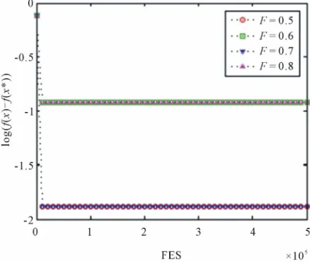
13 and 14. From Figures 13 and 14, we can observe that GNO2DE can achieve the convergence for each value of the above control parameter F when the number of fitness evaluations is set to 100,000 FES, while the convergence speed is fastest when the value of the control parameter F is set to 0.5. For function f₅, we set the

control parameter F to 0.5, 0.6, 0.7, and 0.8, respec-

tively. The convergence graph is given in Figure 15.

From Figure 15, it is clearly shown that the convergence speed is obviously fastest when the value of the control parameter F is set to 0.6. In addition, we also present

the convergence graph of each function of f8, f13, and 20

f in Figures 16-18, respectively. The control parame-

ter F is set to 0.5, 0.6, 0.7, and 0.8. From these figures,

[image:7.595.60.283.359.526.2]

(8)

[image:8.595.58.285.7.775.2] [image:8.595.60.286.81.278.2]

Figure 7. Convergence graph for functions f1- f4.

[image:8.595.312.534.86.272.2]

[image:8.595.310.531.303.494.2]

Figure 10. Convergence graph for functions f13 - f16.

Figure 11. Convergence graph for functions f17 - f20.

[image:8.595.56.283.464.707.2] [image:8.595.313.534.531.716.2]

(9)

[image:9.595.60.286.85.268.2] [image:9.595.311.533.86.269.2]

Figure 13. Convergence curve of f1 for each F value.

[image:9.595.311.532.305.494.2]

[image:9.595.60.284.306.492.2] [image:9.595.59.279.528.714.2] [image:9.595.313.533.530.716.2]

(10)

Therefore, for the most functions, GNO2DE can show good performance when the value of the control parameter F is set to 0.5 or 0.6. According to the above dis-

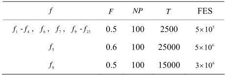
cussion and analysis, we set up the corresponding experimental parameters in Tables 2-4. Table 2 presents the parameters used by GNO2DE, GNO2DE-A, and GNO2DE-B for functions of dimensionality 30 or lower, where GNO2DE-A and GNO2DE-B employ only DE schemes “DE/rand/1/bin” or “DE/current to best/2/bin”, respectively. Table 3 presents the parameters used by GNODE (without using the opposite point method) for functions of dimensionality 30 or lower. Table 4 presents the parameter settings used by GNO2DE for functions of dimensionality 100.

4.3. Comparison of GNO2DE with GNODE

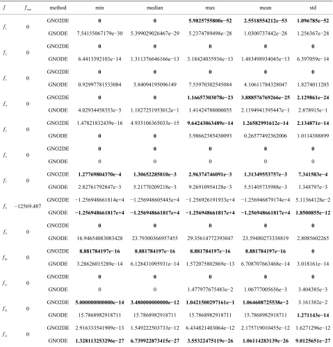
In this section, we compare GNO2DE with GNODE in terms of some performance indices according to the parameter settings presented in Tables 2 and 3. The experimental results are in detail summarized in Tables 5 and 6, and better results are highlighted in boldface. The optimized objective function values over 30 independent runs are arranged in ascending order and the 15th_{value in} the list is called the median optimized function value.

[image:10.595.60.286.431.506.2]

According to Tables 5 and 6, we can find that GNO2DE

Table 2. Parameters used by GNO2DE, GNO2DE-A, and GNO2DE-B for functions of dimensionality 30 or lower.

f F NP T FES

1 - 4

f f , f6, f7, f9 - f23 0.5 100 500 1 10 5

5

f 0.6 100 5000 _{1 10}_ 6

8

[image:10.595.60.285.545.620.2]

f 0.5 100 1500 _{3 10}_ 5

Table 3. Parameters used by GNODE for functions of di- mensionality 30 or lower.

f F NP T FES

1 - 4

f f , f6, f7, f9 - f23 0.5 100 1000 1 10 5

5

f 0.6 100 10000 _{1 10}_ 6

8

f 0.5 100 3000 _{3 10}_ 5

Table 4. Parameters used by GNO2DE for functions of di- mensionality 100.

f F NP T FES

1 - 4

f f , f6, f7, f9 - f23 0.5 100 2500 5 10 5

5

f 0.6 100 25000 _{5 10}_ 6

8

f 0.5 100 15000 _{3 10}_ 6

can obtain the optima or near optima with certain preci- sion for all test functions f1 - f23 of dimensionality 30 or less. For each function of f1 - f4, f6, f7, f9 - f11,

14

f , f₁₅, f₁₇ - f₁₉, and f₂₁ - f₂₃, the performance of

GNO2DE is superior to or less worse than the performance of GNODE in terms of the min value (i.e., the best result), the median value (i.e., the median result), the max value (i.e., the worst result), the mean value (i.e., the mean result), and the std value (i.e., the standard deviation result), on condition that while the FES of GNO2DE is essentially less than that of GNODE, although they are apparently set to the same FES 100,000. In addition, the

global optimum of function f18 found by GNO2DE is

f18(x) = 2.99999999999992, the corresponding x =

(0.00000000061668, −0.99999999932877).

According to Table 5, for f5, the performance of GNO2DE is obviously better than that of GNODE in terms of the max, mean, and std values, while the performance of GNODE is slightly better than that of

GNO2DE in terms of the min, median values. For f8,

the median, max, mean, and std values of GNODE are better than those of GNO2DE, while the min value of

GNODE is approximate to that of GNO2DE. For f12,

the min, median, max, and mean values of GNO2DE are better than those of GNODE, while the std value of GNO2DE is worse than that of GNODE. The reason is that GNO2DE can’t find the optimal solution in very few runs of 30 runs. For function f₁₃, the min, median, max,

mean, and std values of GNO2DE are slightly worse than those of GNODE.

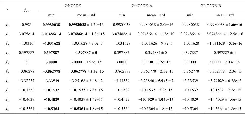
As shown in Table 6, for f16, the min, median values of GNO2DE are similar to those of GNODE, while the max, mean, and std values of GNO2DE are worse than those of GNODE to some extent. This is because that GNO2DE can’t obtain the min value in one or two runs of 30 runs. For f20, the min, and max values obtained by GNO2DE are the same to those by GNODE, while the median value obtained by GNO2DE is worse than that obtained by GNODE. Accordingly, it also decides that the mean, and std values of GNO2DE are worse than those of GNODE. GNO2DE and GNODE all have a tendency to getting stuck in the local optima. The global optima of function f20 found by GNO2DE is f20(x) =

−3.33539215295525, the corresponding

x = (0.20085810809731, 0.15013171771783,

0.47865329178970, 0.27652528463205, 0.31191293322300, 0.65702016661775).

[image:10.595.56.286.658.735.2]

(11)

[image:11.595.60.539.105.605.2]

Table 5. Comparison between GNO2DE, and GNODE on functions f1- f13 of dimensionality 30.

f fmin method min median max mean std

GNO2DE 0 0 5.9825755800e−52 2.5518554212e−53 1.096785e−52

1

f 0

GNODE 7.54155067179e−30 5.399029026467e−29 5.2374789498e−28 1.0300737442e−28 1.256367e−28

GNO2DE 0 0 0 0 0

2

f 0

GNODE 6.4413392103e−14 1.311376646166e−13 3.18424035936e−13 1.483498934045e−13 6.397059e−14

GNO2DE 0 0 0 0 0

3

f 0

GNODE 0.92997781533084 3.84094195096149 7.55970302545084 4.10611784328047 1.8274011203

GNO2DE 0 0 1.16657303078e−23 3.888576769266e−25 2.129861e−24

4

f 0

GNODE 4.02934458353e−3 1.1827251953012e−1 1.41424788000055 2.1194941395447e−1 2.878915e−1

GNO2DE 1.47821832439e−16 4.935106365033e−15 9.64243063489e−14 1.26582991612e−14 2.134871e−14

5

f 0

GNODE 0 0 3.98662385430093 0.26577492362006 1.0114388899 GNO2DE 0 0 0 0 0

6

f 0

GNODE 0 0 0 0 0

GNO2DE 1.27769804370e−4 1.30652285810e−3 2.96374746091e−3 1.31349553757e−3 7.341583e−4

7

f 0

GNODE 2.82761792847e−3 5.21770209218e−3 9.26910954128e−3 5.51405735988e−3 1.348797e−3

GNO2DE −1.256948661814e+4 −1.256948605445e+4 −1.256926191933e+4 −1.256946879174e+4 5.11364128e−2

8

f −12569.487

GNODE −1.256948661817e+4 −1.256948661817e+4 −1.256948661817e+4 −1.256948661817e+4 1.8500855e−12

GNO2DE 0 0 0 0 0

9

f 0

GNODE 16.94654083083428 23.79300366957455 29.35614772393047 23.59480273338819 2.8085602265

GNO2DE 8.881784197e−16 8.881784197e−16 8.881784197e−16 8.881784197e−16 0

10

f 0

GNODE 3.28626015289e−14 6.128431095931e−14 1.572075802869e−13 6.708707663468e−14 3.018161e−14

GNO2DE 0 0 0 0 0

11

f 0

GNODE 0 0 1.477977675483e−2 1.06777005656e−3 3.404385e−3

GNO2DE 5.000000000000e−14 3.480000000000e−12 1.0421500297161e−1 1.064608725538e−2 3.161382e−2

12

f 0

GNODE 15.7868982918711 15.7868982918711 15.7868982918711 15.7868982918711 1.271143e−14

GNO2DE 2.916333541909e−13 1.549222503733e−12 6.434821403064e−12 2.175719010455e−12 1.6271296e−12

13

f 0

GNODE 1.328113253296e−27 6.739922873415e−27 3.55322475119e−26 1.06114283139e−26 9.0125651e−27

4.4. Comparison of GNO2DE with GNO2DE-A, and GNO2DE-B

In this section, we compare GNO2DE (“DE/rand/1/bin” and “DE/current to best/2/bin”) with GNO2DE-A (“DE/ rand/1/bin”), and GNO2DE-B (“DE/current to best/2/ bin”) in terms of the best result (i.e., the min value), the mean result (i.e., the mean value), and the standard deviation result (i.e., the std value). The parameter settings of GNO2DE, GNO2DE-A, and GNO2DE-B are given in

Table 2. The experimental results are in detail summarized in Tables 7 and 8, and better results are highlighted in boldface. The optimized objective function values over 30 independent runs are arranged in ascending order and the 15th_{value in the list is called the median} opti-mized function value.

From Tables 7 and 8, it is clearly shown that for each function of f6, f9 - f11, f14, f17 - f23, the min, mean,

(12)

[image:12.595.59.539.105.466.2]

Table 6. Comparison between GNO2DE, and GNODE on functions f14 - f23.

f fmin method min median max mean std

GNO2DE 0.99800383779445 0.99800383779445 0.99800383779445 0.99800383779445 1.749353e−16

14

f 0.998

GNODE 0.99800383779445 0.99800383779445 0.99800383779445 0.99800383779445 1.129203e−16

GNO2DE 3.074859878056e−4 3.074859878056e−4 3.074859878056e−4 3.074859878056e−4 1.318374e−18

15

f 3.075e−4

GNODE 3.074859878056e−4 3.074859878056e−4 3.074859878056e−4 3.074859878056e−4 1.055790e−19

GNO2DE −1.03162845348988 −1.03162845348988 −1.03162683969173 −1.03162838522757 3.024594e−7

16

f −1.0316

GNODE −1.03162845348988 −1.03162845348988 −1.03162845348988 −1.03162845348988 6.775215e−16

GNO2DE 0.39788735772974 0.39788735772974 0.39788735772974 0.39788735772974 0

17

f 0.397887

GNODE 0.39788735772974 0.39788735772974 0.39788735772974 0.39788735772974 0

GNO2DE 2.99999999999992 2.99999999999992 2.99999999999992 2.99999999999992 1.953227e−15

18

f 3

GNODE 2.99999999999992 2.99999999999992 2.99999999999992 2.99999999999992 1.989449e−15 GNO2DE −3.86277751253760 −3.86277751253760 −3.86277751253760 −3.86277751253760 2.258405e−15

19

f −3.86278

GNODE −3.86277751253760 −3.86277751253760 −3.86277751253760 −3.86277751253760 2.258405e−15 GNO2DE −3.33539215295525 −3.20321215577107 −3.20321215577107 −3.25167815473861 6.478571e−2

20

f −3.32237

GNODE −3.33539215295525 −3.33539215295525 −3.20321215577107 −3.27811415417544 6.661963e−2 GNO2DE −10.15319967905823 −10.15319967905823 −10.15319967905823 −10.15319967905822 7.226896e−15

21

f −10.1532

GNODE −10.15319967905823 −10.15319967905823 −5.10077214033199 −9.81637117647648 1.281841951 GNO2DE −10.40294056681867 −10.40294056681867 −10.40294056681866 −10.40294056681866 1.615983e−15

22

f −10.4029

GNODE −10.40294056681867 −10.40294056681867 −10.40294056681866 −10.40294056681866 1.714009e−15 GNO2DE −10.53640981669205 −10.53640981669205 −10.53640981669205 −10.53640981669205 1.776357e−15

23

f −10.5364

GNODE −10.53640981669205 −10.53640981669205 −10.53640981669205 −10.53640981669205 1.806724e−15

GNO2DE-A, and GNO2DE-B, and three algorithms all can find the optimal solution.

Table 7 shows that for each function of f1- f4, the optimal solution can be found by GNO2DE, GNO2DE-A, and GNO2DE-B, while the mean, std values of GNO2DE are slightly different from those of GNO2DE-A, and

GNO2DE-B. For f5, the mean, and std values of

GNO2DE are obviously better than those of GNO2DE-A, and GNO2DE-B, while the min value of GNO2DE-A is worst among three algorithms. For f7, the min value of GNO2DE-A is best among three algorithms, while its mean, and std values are worse or not better than those of

GNO2DE, and GNO2DE-B. For f₈, the min, mean, and

std values of GNO2DE-B are obviously worse than those of GNO2DE, and GNO2DE-A, while GNO2DE-A can obtained better mean, and std values than GNO2DE. For

12

f , the min value of GNO2DE-A is worst among three

algorithms, while the std value of GNO2DE is best

among three algorithms. For f13, the min value of

GNO2DE-A is worst among three algorithms, while the mean, and std values of GNO2DE are best among three

algorithms.

Table 8 shows that for f15, the min, and mean values are approximate among three algorithms, while the std value of GNO2DE is best, that of GNO2DE-B is better,

and that of GNO2DE-A is good. For f16, the min, and

mean values are similar among three algorithms, while the std value of GNO2DE-B is best, that of GNO2DE is better, and that of GNO2DE-A is good.

Therefore, from the above analysis, we know that the performance of GNO2DE is more stable than that of GNO2DE-A, and that of GNO2DE-B. This is because that GNO2DE employs two schemes “DE/bin/1/bin” and “DE/current to best/2/bin” to search the solution space. On the whole, GNO2DE can improve the search ability.

4.5. Comparison of GNO2DE with Some State-of-the-Art Algorithms

(13)

[image:13.595.59.538.106.385.2]

Table 7. Comparison between GNO2DE, GNO2DE-A, and GNO2DE-B on functions f1- f14 of dimensionality 30.

GNO2DE GNO2DE-A GNO2DE-B f fmin

min mean ± std min mean ± std min mean ± std

1

f 0 0 2.55e−53 ± 1.1e−52 0 0 ± 0 0 4.2e−59 ± 1.6e−58

2

f 0 0 0 ± 0 0 0 ± 0 0 2.1e−34 ± 1.2e−33

3

f 0 0 0 ± 0 0 0 ± 0 0 2.8e−54 ± 1.5e−53

4

f 0 0 3.89e−25 ± 2.13e−24 0 0 ± 0 0 1.3e−23 ± 3.26e−23

5

f 0 1.4782e−16 1.2658e−14 ± 2.1e−14 4.3857 5.414 ± 4.4e−1 0.0000 4.6295 ± 5.0103

6

f 0 0 0 ± 0 0 0 ± 0 0 0 ± 0

7

f 0 1.2777e−4 1.3135e−3 ± 7.3e−4 5.3502e−5 1.3537e−3 ± 1.2e−3 1.3892e−4 9.3933e−4 ± 4.2e−4

8

f −12569.487 −12569.487 −12569.469 ± 5.2e−2 −12569.487 −12569.487 ± 2.3e−5 −12230.228 −11423.429 ± 3.7e+2

9

f 0 0 0 ± 0 0 0 ± 0 0 0 ± 0

10

f 0 8.8818e−16 8.8818e−16 ± 0 8.8818e−16 8.8818e−16 ± 0 8.8818e−16 8.8818e−16 ± 0

11

f 0 0 0 ± 0 0 0 ± 0 0 0 ± 0

12

f 0 5.0000e−14 1.0646e−2 ± 3.16e−2 1.9663e−5 8.4895e−2 ± 1.25e−1 0 2.0875e−2 ± 1.13e−1

13

f 0 2.9163e−13 2.1757e−12 ± 1.6e−12 1.8552e−5 9.3345e−4 ± 5.87e−4 0 1.7522e−3 ± 4.8e−3

Table 8. Comparison between GNO2DE, GNO2DE-A, and GNO2DE-B on functions f14 - f23.

GNO2DE GNO2DE-A GNO2DE-B f fmin

min mean ± std min mean ± std min mean ± std

14

f 0.998 0.9980038 0.9980038 ± 1.7e−16 0.9980038 0.9980038 ± 2.0e−16 0.9980038 0.9980038 ± 1.6e−16

15

f 3.075e−4 3.07486e−4 3.07486e−4 ± 1.3e−18 3.07486e−4 3.07486e−4 ± 1.3e−10 3.07486e−4 3.07486e−4 ± 2.5e−16

16

f −1.0316 −1.031628 −1.031628 ± 3.0e−7 −1.031628 −1.031626 ± 9.9e−6 −1.031628 −1.031628 ± 5.1e−16

17

f 0.397887 0.397887 0.397887 ± 0 0.397887 0.397887 ± 0 0.397887 0.397887 ± 0

18

f 3 3.0000 3.0000 ± 1.95e−15 3.0000 3.0000 ± 1.7e−15 3.0000 3.0000 ± 2.03e−15

19

f −3.86278 −3.862778 −3.862778 ± 2.3e−15 −3.862778 −3.862778 ± 2.3e−15 −3.862778 −3.862778 ± 2.3e−15

20

f −3.32237 −3.33539 −3.25168 ± 6.48e−2 −3.33539 −3.23846 ± 5.945e−2 −3.33539 −3.29029 ± 6.28e−2

21

f −10.1532 −10.1532 −10.1532 ± 7.2e−15 −10.1532 −10.1532 ± 7.2e−15 −10.1532 −10.1532 ± 7.2e−15

22

f −10.4029 −10.4029 −10.4029 ± 1.6e−15 −10.4029 −10.4029 ± 1.04e−15 −10.4029 −10.4029 ± 1.6e−15

23

f −10.5364 −10.5364 −10.5364 ± 1.8e−15 −10.5364 −10.5364 ± 1.8e−15 −10.5364 −10.5364 ± 1.8e−15

number of fitness evaluations (i.e., the FES value). The statistical results are summarized in Tables 9 and 10, and better results are highlighted in boldface. The experimental results of DE, SOA, and CLPSO are taken from [31], and the experimental results of ODE/2, FEP are taken from [2]. The optimized objective function values of 30 runs are arranged in ascending order and the 15th

[image:13.595.57.538.415.640.2]

(14)

[image:14.595.63.536.126.737.2]

Table 9. Comparison between GNO2DE, DE, ODE/2, SOA, FEP, opt-IA, and CLPSO on functions f1 - f14 of dimensiona-

lity 30.

opt-IA f item GNO2DE DE ODE/2 SOA FEP

 *f

e 

_  1  f

e

 



 

  _{ } CLPSO

mean 2.5519e−53 3.74e−13 2.06e−23 1.02e−76 5.7e−4 9.23e−12 1.7e−8 2.73e−12 std 1.0968e−52 3.94e−13 1.83e−23 6.51e−76 1.3e−4 2.44e−11 3.5e−15 1.68e−12

1

f

FES 100,000 150,000 150,000 150,000 150,000 150,000 150,000 150,000 mean 0 3.74e−9 1.43e−18 4.22e−63 8.1e−3 0.0 7.1e−8 3.82e−9

std 0 2.20e−9 8.11e−19 8.25e−63 7.7e−4 0.0 0.0 1.73e−9

2

f

FES 100,000 200,000 200, 000 200,000 200,000 200,000 200,000 200,000 mean 0 1.85e−10 5.25e−27 4.26e−25 1.6e−2 0.0 1.9e−10 4.20e−1

std 0 1.49e−10 9.66e−27 2.15e−24 1.4e−2 0.0 2.63e−10 3.62e−1

3

f

FES 100,000 500,000 500,000 500,000 500,000 500,000 500,000 500,000 mean 3.8886e−25 3.10e−2 2.72e−15 1.02e−48 0.3 1.0e−2 4.1e−2 2.05e−3

std 2.1299e−24 8.70e−2 9.30e−15 2.46e−48 0.5 5.3e−3 5.3e−2 1.25e−3

4

f

FES 100,000 500,000 500,000 500,000 500,000 500,000 500,000 500,000 mean 1.2658e−14 3.47e−31 0 2.54e+1 5.06 3.02 28.4 3.63e+1

std 2.1349e−14 2.45e−30 0 7.87e−1 5.87 12.2 0.42 3.12e+1

5

f

FES 1000,000 2000,000 428,776 2000,000 2000,000 2000,000 2000,000 2000,000 mean 0 0 0 0 0 0,2 0.0 0

std 0 0 0 0 0 0.44 0.0 0

6

f

FES 100,000 150,000 22,640 150,000 150,000 150,000 150,000 150,000 mean 1.3135e−3 4.66e−3 1.45e−3 1.08e−4 7.6e−3 3.0e−3 3.9e−3 2.98e−3

std 7.3416e−4 1.30e−3 4.20e−4 6.44e−5 2.6e−3 1.2e−3 1.3e−3 9.72e−4

7

f

FES 100,000 300,000 300,000 300,000 300,000 300,000 300,000 300,000 mean −12569.4688 −11234 −12569.4866 −10126 −12554.5 −12508.38 −12568.27 −12271

std 5.1136e−2 455.5 0 669.5 52.6 155.54 0.23 177.8

8

f

FES 300,000 900,000 90, 381 900,000 900,000 900,000 900,000 900,000 mean 0 8.10e+1 0 0 4.6e−2 19.98 2.66 1.34e−9

std 0 3.23e+1 0 0 1.2e−2 7.66 2.39 8.57e−10

9

f

FES 100,000 500,000 127,666 500,000 500,000 500,000 500,000 500,000 mean 8.8818e−16 1.71e−7 4.67e−13 −4.44e−15 1.8e−2 18.98 1.1e−4 6.81e−6

std 0 7.66e−8 1.86e−13 0 2.1e−3 0.35 3.1e−5 1.94e−6

10

f

FES 100,000 150,000 150,000 150,000 150,000 150,000 150,000 150,000 mean 0 4.44e−4 0 0 1.6e−2 7.7e−2 4.55e−2 2.96e−4

std 0 1.77e−3 0 0 2.2e−2 8.63e−2 4.46e−2 1.46e−3

11

f

FES 100,000 200,000 109, 853 200,000 200,000 200,000 200,000 200,000 mean 1.0646e−2 3.67e−14 6.73e−26 1.28e−2 9.2e−6 0.137 3.1e−2 4.80e−11

std 3.1614e−2 4.07e−14 9.27e−26 7.62e−3 3.6e−6 0.23 5.7e−2 3.96e−11 2

1 f

FES 100,000 150,000 150,000 150,000 150,000 150,000 150,000 150,000 mean 2.1757e−12 2.91e−13 4.37e−24 1.89e−1 1.6e−4 1.51 3.20 6.42e−10

std 1.6271e−12 2.88e−13 3.67e−24 1.30e−1 7.3e−5 0.10 0.13 4.46e−10 3

1 f

(15)

[image:15.595.62.535.104.672.2]

Table 10. Comparison between GNO2DE, DE, ODE/2, SOA, FEP, opt-IA, and CLPSO on functions f14 - f23.

opt-IA f item GNO2DE DE ODE/2 SOA FEP

 *f

e 

_  1  f

e

 



 

  _{ } CLPSO

mean 0.9980038 0.998 0.998 1.199 1.22 1.02 1.21 0.998 std 1.7494e−16 2.88e−16 0 5.30e−1 0.56 7.1e-2 0.54 5.63e−10

14

f

FES 100,000 10,000 9552 10,000 10,000 10,000 10,000 10,000 mean 3.07486e−4 4.7231e−2 3.08e−4 3.0749e−4 5.0e−4 7.1e−4 7.7e−3 5.3715e−4

std 1.3184e−18 3.55e−4 0 1.58e−9 3.2e−4 1.3e−4 1.4e−2 6.99e−5

15

f

FES 100, 000 400, 000 32,430 400, 000 400, 000 400, 000 400, 000 400, 000 mean −1.031628 −1.0316 −1.03163 −1.0316 −1.031 −1.03158 −1.02 −1.0316 std 3.0246e−7 6.77e−13 0 6.73e−6 4.9e−7 1.5e−4 1.1e−2 8.50e−14

16

f

FES 100,000 10,000 10,000 10,000 10,000 10,000 10,000 10,000 mean 0.397887 0.39789 0.39789 0.39838 0.398 0.398 0.450 0.39789

std 0 1.14e−8 2.01e−10 5.14e−4 1.5e−7 2.0e−4 0.21 1.08e−13

17

f

FES 100,000 10,000 10,000 10,000 10,000 10,000 10,000 10,000

mean 3.0000 3 3.00 3.0001 3.02 3.0 3.0 3 std 1.9532e−15 3.31e−15 0 1.17e−4 0.11 0.0 0.0 5.54e−13

18

f

FES 100,000 10,000 10,000 10,000 10,000 10,000 10,000 10,000 mean −3.8627775 −3.8628 −3.86278 −3.8621 −3.86 −3.72 −3.72 −3.8628

std 2.2584e−15 1.97e−15 2.68e−15 6.69e−4 1.4e−5 1.1e−4 1.1e−2 6.07e−12

19

f

FES 100,000 10,000 10,000 10,000 10,000 10,000 10,000 10,000 mean −3.251678 −3.215 −3.322 −3.298 −3.27 −3.31 −3.31 −3.274

std 6.4786e−2 3.6e−2 1.13e−12 4.5e−2 5.9e−2 7.4e−2 5.9e−3 5.9e−2

20

f

FES 100, 000 20, 000 20,000 20, 000 20,000 20,000 20,000 20,000 mean −10.1531997 −10.15 −10.1532 −9.67 −5.52 −9.11 −5.36 −9.57 std 7.2269e−15 4.67e−6 1.04e−6 4.96e−1 1.59 1.82 2.20 4.28e−1

21

f

FES 100,000 10,000 10,000 10,000 10,000 10,000 10,000 10,000 mean −10.40294 −10.40 −10.40294 −9.79 −5.52 −9.86 −5.34 −9.40

std 1.61598e−15 2.07e−7 2.49e−8 4.48e−1 2.12 1.88 2.11 1.12

22

f

FES 100,000 10,000 10,000 10,000 10,000 10,000 10,000 10,000 mean −10.5364098 −10.54 −10.53641 −9.72 −6.57 −9.96 −6.03 −9.47

std 1.7764e−15 3.21e−6 2.35e−8 4.72e−1 3.14 1.46 2.66 1.25

23

f

FES 100,000 10,000 10,000 10,000 10,000 10,000 10,000 10,000

4

f , f₇, while the 100,000 FES of GNO2DE is least

among these methods, and that the mean, std, FES values of GNO2DE are better than DE, ODE/2, FEP, opt-IA, and CLPSO. For f5, f6, f8, the mean, std, and FES

values of ODE/2 are not worse than or better than those

of other methods. For f5, compared with DE, GNO2DE

(16)

GNO2DE, and the performance of GNO2DE is clearly better than that of SOA, FEP, opt-IA, and CLPSO. For

6

f , the mean, std values of GNO2DE are similar to those

of DE, SOA, FEP, opt-IA, and CLPSO, while the 100,000 FES used by GNO2DE is least among these

methods. For f8 , the mean, std, FES values of

GNO2DE are obviously better than those of DE, SOA, FEP, opt-IA, and CLPSO. For f12, f13, the min, std values of ODE/2 are better than those of other methods, while the 100,000 FES used by GNO2DE is least among these methods.

As shown in Table 10, the mean value of GNO2DE

and SOA on f15 is approximate and are better than oth-er methods, while ODE/2 has the least std, and FES val-ues. For f16 - f18, all methods have the similar per-

for-mance. For f19, GNO2DE, DE, ODE/2, SOA, CLPSO

have the similar performance and are better than FEP.

For f20, the performance of ODE/2 and FEP is better

than other methods. For f21 - f23, the performance of GNO2DE, DE, and ODE/2 is approximate and are better than other methods.

In sum, the mean and standard deviation results of GNO2DE are not worse than or superior to DE, ODE/2, SOA, FEP, opt-IA, and CLPSO on a test set of benchmark functions. GNO2DE uses the opposite point method, employs two DE schemes “DE/rand/1/bin” and “DE/ current to best/2/bin”, and introduces non-uniform crossover rate. These techniques are beneficial to enhancing the performance of GNO2DE.

4.6. Experimental Results of 100-Dimensional Functions

In this section, the statistical results of GNO2DE on 100-

dimensional functions are given in Table 11. The pa-

rameter setup is used in Table 4. The optimized object- tive function values over 30 independent runs are arranged in ascending order and the 15th_{value in the list is}

called the median optimized function value. Table 11

clearly shows that GNO2DE can find the optimum or near optimum of each 100-dimensional function of f1- f13, and that GNO2DE can obtain the stable performance of each function of f1- f7, f9 - f11, while it performs slightly worse on f8, f12, f13. Therefore, when used for solving high dimensional global numerical optimization problems, NGO2DE also performs well.

5. Conclusion and Future Work

[image:16.595.56.540.467.731.2]

This paper introduces an opposition-based DE algorithm for global numerical optimization (GNO2DE). GNO2DE uses the method of opposition-based learning to utilize the existing search spaces to improve the convergence speed, employs adaptive DE schemes and non-uniform crossover to enhance the adaptive search ability. Nume- rical results show that GNO2DE outperforms some state- of-the-art algorithms. However, there are still some possible things to do in the future: 1) further, to improve the self-adaptation of the control parameters such as the scaling factor F; 2) to test higher dimensional global nu-

Table 11. Experimental Results of 100-dimensional functions f1- f13.

f fmin min median max mean std FES

1

f 0 0 0 0 0 0 _{5 10}_ 5

2

f 0 0 0 0 0 0 _{5 10}_ 5

3

f 0 0 0 0 0 0 _{5 10}_ 5

4

f 0 0 0 0 0 0 _{5 10}_ 5

5

f 0 3.497698e−19 7.195169e−18 5.756444e−15 4.662977e−16 1.318697e−15 _{5 10}_ 6